Quantitative Calibration of Remote Mountain-Lake Sediments as Climatic Recorders of Air Temperature and Ice-Cover Duration

Abstract

A combination of empirical modeling and a diatom-based transfer function was developed to reconstruct air temperature and ice-cover duration through the study of lake sediments. By using a thermal degree-day modeling approach, ice-cover duration on European mountain and sub-Arctic lakes is found to be very sensitive to temperature change. For example, our model, which incorporates a weather generator, predicts a 100-day shortening in ice-cover duration for a 3°C temperature rise for catchments at elevations of 1500 m in the Southern Alps and the Pyrenees. For the more maritime lakes of Scotland, 30% higher sensitivities (130 d per 3°C) are found, whereas lakes in northwest Finland, in a more continental setting, have only half the sensitivity (50 d per 3°C). A pan-European data set of the species abundance of 252 diatom taxa in 459 mountain and sub-Arctic lakes has been compiled and taxonomically harmonized. Transfer functions were created that relate both seasonal air temperature and ice-cover duration to diatom species composition on the basis of a weighted averaging–partial least squares (WA-PLS) approach. Cross validation was used to test the transfer functions. For ice-cover duration the pan-European data set yields an R-squared value of 0.73, a jack-knifed R-squared value of 0.58, and a residual-mean-square error of prediction (RMSEP) of 23 days. A regional, northern Fennoscandian transect (151 lakes, 122 taxa) yields a jack-knifed R-squared value of 0.50 and an RMSEP of 9 days. For air temperature the pan-European database displayed greatest skill when reconstructing winter or spring temperatures. This result contrasts with the summer temperatures normally studied when using local elevation gradients. The northern Fennoscandian transect has a remarkably low winter RMSEP of 0.73°C.

Introduction

REMOTE LAKES

Lakes at high altitude and high latitude are expected to be very sensitive to global warming and climate change because their biological activity is largely restricted to the duration of their short ice-free season, which is determined by climate. Compilations of historical time series of ice cover point to later freezing and earlier ice-breakup dates for lakes and rivers in the Northern Hemisphere over the past 150 yr (Magnuson et al., 2000). This trend is expected to continue into the future as the climate becomes warmer (Burn and Hag Elnur, 2002). Many important processes in mountain lakes are closely related to ice-cover duration. For example lake stratification is strongly controlled by ice cover. Following ice breakup, as a mountain lake mixes in the spring, the phosphorus and ammonium that has built up in the bottom water during the winter circulates and fuels increased algal growth. In alpine lakes, biological activity peaks during this spring mixing and again later in the summer as photosynthetic activity is driven by high solar radiation. In high-latitude lakes the production maximum occurs usually during the autumnal circulation period (Sorvari et al., 2000). In summary, remote lakes have high potential as natural monitors and recorders of past climatic change because (1) their biological activity is closely coupled to the physical properties of stratification and ice cover, which in turn are directly controlled by climatic dynamics, and (2) their fossil record has been little disturbed by human activities.

AIR TEMPERATURE AND ICE COVER

Mountain-lake sediments have proved to be excellent recorders of pollution and environmental change (Battarbee et al., 2002). Quantitative reconstructions of past changes can be made by using transfer functions that match the present-day geographical variation of a parameter (e.g., pH) with the fossil assemblages preserved in surface sediments. Within a lake, pH variations from month to month and place to place are modest. Consequently for lake-sediment–based transfer-function work, a few measurements of the pH of the lake water suffices. By contrast, individual observations of ice-cover duration are by themselves not sufficient for calibration purposes. Instead, we need to develop a model that will allow ice-cover duration to be inferred at any remote lake site. Year-by-year changes can then be allowed for, and robust estimates of ice-cover duration can be established that span the interval of time during which the uppermost sediment was deposited (typically 5–10 yr). Comparisons can then be made with the concentrations of fossil organisms preserved in the surficial sediments.

Ice cover and air temperature are closely linked. However, many physical processes are involved in their relationship. These include the cooling of the lake waters in autumn by radiative losses to the air, evaporative cooling, and stream outflow. During winter months the snow cover and ice albedo are also of importance to the temperature balance. Conduction from the atmosphere, condensation of water vapor, and inflows of stream runoff and groundwater are other significant processes. Thus, even one-dimensional thermodynamic ice-cover models require a number of meteorological variables as input. These include daily mean air temperature, wind speed, relative humidity, cloud cover, snow depth, and snow density (Stefan and Fang, 1997).

Although many physical processes control water temperature and ice cover, simple empirical models based solely on air temperature can be constructed to represent their behavior (Kettle et al., 2004; Bilello, 1964). Here a thermal degree-day modeling approach to ice-cover duration is employed. We use it in three applications: (1) to explore the sensitivity of the ice cover of mountain lakes to air temperature, (2) to predict future changes in ice cover on mountain lakes due to global warming, and (3) to investigate the potential for reconstructing past climatic changes by use of a diatom vs. ice-cover transfer function based on lake sediment data. Daily air temperatures, at each lake studied, are needed to “drive” the ice-cover model. Fortunately, time series of daily air temperature are spatially highly coherent, even in mountain regions (Jones and Thompson, 2003). So air temperatures at mountain lakes can be estimated either from observations at lowland stations through the use of regression methods (Agusti-Panareda and Thompson, 2002) or from reanalysis assimilations of the state of the atmosphere by using downscaling procedures (Kettle and Thompson, 2004).

DIATOMS

The pioneering studies of Kolbe (1927) and Hustedt (1927–1966) first demonstrated the great potential and utility of diatom algal floras as indicators of environmental conditions. They were able to develop a system of classification and indices for salinity and lake-water pH based on the relationships of diatoms and water chemistry as found across a wide range of habitats. Most microbes do not grow (easily) under laboratory conditions, so the preferred method of establishing the response and tolerance of the hundreds of diatom taxa to be found in mountain freshwater systems remains—to paraphrase Deevey (1969)—as one of “coaxing nature to conduct experiments for you.” In studies of the diatom flora of mountain lakes, elevation gradients (i.e., staircases of lake basins down the flanks of mountain ranges) have provided a means of establishing the relationship of diatom assemblages to temperature and climate. Several attractive-looking relationships (e.g., Lotter et al., 1997; Weckström et al., 1997; Rosén et al., 2000; Bigler and Hall, 2002) have been established by using elevation gradients. One drawback with using local elevation gradients is that many environmental factors tend to covary as one ascends through the upper forests, past the treeline, and on through the alpine zone to the snowline. Maximum summer temperatures decrease; as do winter, spring, and autumn temperatures. Precipitation, nutrient supply, and water-quality commonly display similar monotonic trends. As a consequence, problems with latent variables and collinearity—those well-known banes of multiple regression techniques—raise their ugly heads. Is there any escape from the numerical problems emanating from collinearity, or near collinearity, that would seem inevitable in elevation gradient work? Here we explore the effect of combining elevation gradients from across Europe. A potential advantage is that the larger array of lake sites will populate an enlarged volume of “climate space” and so reduce the numerical problems associated with near collinearity that lead to inaccurate estimates of regression coefficients, variability, and significance levels. Such an advantage must be weighed against the disadvantages of reduced taxonomic harmony and greater within-species genetic diversity that will inevitably be associated with a pan-continental study. Resampling techniques, e.g., leave-one-out-at-a-time cross-validation, provide us with a formal mechanism for assessing the virtue of employing a pan-European training set of lake basins.

BIOLOGICAL TRANSFER FUNCTION

Inferring environmental variables from micropaleontological assemblages is a difficult multivariate calibration problem, and a variety of numerical techniques have been proposed for its solution. In paleoceanography, a form of principal components regression is frequently used. In paleolimnology, the method of weighted averaging (WA) has gained considerable support and appears to be particularly suited to the noisy, species-rich, compositional data that characterize diatom training sets. We follow the widely used weighted averaging approach. Ideally, for skilful reconstruction work, the set of present-day lakes under study should span the complete range of conditions that are likely to have been present in the past; the biological proxy should encompass a wide ensemble of species, not only in the whole set, but also in each individual lake; and the target climate parameter should not be biased by local effects involving specific features of individual lakes or catchments.

Materials and Methods

CLIMATE DATA

Climate data (maximum, minimum, and mean air temperatures) as measured at WMO (World Meteorological Organization) stations were taken from the CRU (Climate Research Unit) (www.cru.uea.ac.uk/cru/data) and NOAA (U.S. National Oceanic and Atmospheric Administration) databases (www.ncdc.noaa.gov/pub/data). Daily data, from 1994 onward, were used to determine the parameters employed in the weather generator (Fig. 1). A detailed study of the Southern Alps based on daily data at 32 stations was carried out. They stretch geographically from Pianrosa (3488-m elevation) and Turin (287 m) in the west to Sonnblick Mountain (3107 m) and Tarvisio (778 m) in the east, and they range in altitude from Jungfrau Mountain (3576 m) to Venice (53 m). Monthly averages at WMO stations were used in the construction of climate normals for the mountain and sub-Arctic regions of Europe and used in the diatom vs. ice-cover transfer-function work. Upper air data from the Monthly Climate Data for the World (MCDW) data set, as compiled by the U.K. National Climate Data Centre (NCDC), for the period 1990–1998 between 1000 and 500 hPa provided the basic data for lapse-rate determinations.

A well-known meteorological phenomenon that we need to take into account is the “frost-hollow” effect of Alpine valley sites, such as Samedan (1705 m) and Klagenfurt (448 m) Airports. Anomalies of −5°C in monthly mean air temperature, caused by cold air collecting on calm, clear nights, are found in late-autumn to early-winter months (NDJ). This effect is also of great importance in the Scandes Mountains. Frost-hollow sites stand out as isolated anomalies, when compared with the local lapse rate, and have been avoided in our study. Air temperature as recorded by automatic weather stations deployed at mountain-lake sites (Agusti-Panareda and Thompson, 2002) turn out to be predominantly free from the frost-hollow effect. They closely match the local “lapse rate,” and provide a valuable data set for verifying our air-temperature interpolation procedures.

Numerical Procedures

Weather Generator

Weather-generator models are commonly based on Markov chains and autoregressive models of first or higher order (Gabriel and Neumann, 1962; Gates and Tong, 1976; Katz, 1977; Richardson, 1981). Once the parameters of the generator have been derived, from observed weather data, arbitrarily long series with stochastic structure similar to the real data can be generated. To construct time series for changed climate conditions, the parameters of the generator are modified according to the new climate-change scenario (Fig. 1). Here, in order to generate series of daily mean temperatures, we first obtain the characteristics of the mean annual cycle and the interdiurnal variability. The annual cycle is represented by a four-term Fourier series, and the interdiurnal variability is characterized by lag correlations (of order two). That is, we define a second-order autoregression process, AR(2), for a time series X _t by where Z _t , the innovations, are zero-mean, uncorrelated random disturbances. Having already identified the order of the process, by use of both the autocorrelation function (acf) and the partial autocorrelation function (pacf), we then estimated the most likely values of the parameters (the φ variables in equation 1) by maximum likelihood (Ansley, 1979) and AIC (Akaike's information criterion) (Akaike, 1974). A seasonal cycle in the interannual variability of the daily temperature anomalies is also included in our model. We used the fast Fourier transform algorithm, as set out in Bloomfield (1976), to identify the annual cycle and seasonal behavior of our weather generator.

Although the weather generator employed here is really quite simple (mainly because precipitation is not involved), it nevertheless needs 10 parameters at any one locality. Table 1 lists the 10 parameters and their mean rate of change with elevation in the Southern Alps. Figure 2 plots the variation with altitude of four of the parameters for 32 weather stations in the Southern Alps. Similar changes with altitude are found for the other six parameters, and so all 10 elevation trends are incorporated into the final algorithm used for weather generation. For the forecast work a random number generator (Kinderman and Monahan, 1977) was used to provide the innovations in equation 1. These, along with the seasonal structure, were then used to derive 100-yr-long synthetic series of daily mean temperature for present climate conditions and for the changed climate conditions.

Mean Air Temperature

A two-dimensional local regression model (“loess”) was used to interpolate air temperatures from the 0.5° latitude by 0.5° longitude gridded climatology of Hulme and coworkers (Hulme et al., 1995) where air temperature is recorded as monthly means over the period 1961–1990 with a precision of 0.1°C. A local-quadratic fitting of the polynomial was used in the loess-based procedure. In the troposphere, air temperature decreases with increasing altitude, typically at a rate of 6°C km⁻¹, but varying according to altitude, topography, and season. We used upper-air data between 1000 and 500 hPa to estimate the vertical temperature lapse rate for all the mountain ranges studied. These lapse rates, when combined with the loess interpolations, allow monthly air temperatures to be estimated for lakes across the whole of Europe.

The wide geographical spread of the altitudinal gradients used to form our 459-lake training set ensured that it spanned a wide range of temperature regimes. Mean air temperatures varied from −6°C to 8°C, whereas the annual range varied between 10°C and 28°C. Our training set thus embraces the changes in air temperatures that can be expected as a consequence of global warming. Furthermore it can be seen that any errors associated with the loess-based interpolation scheme are likely to be small when compared to the total range of air temperatures we are analyzing.

Ice-Cover Empirical Model

A thermal-degree approach has been implemented as a physically based, empirical model of lake ice-cover duration. The model has only two key parameters. These are the number of freezing degree-days (FDDs) needed to trigger an ice-on event, and the number of melting degree-days (MDDs) needed to trigger an ice-off event. Ice and water have very different physical properties (e.g., albedo) so lake waters freeze more readily than lake ice melts. On account of the differences between these two threshold effects, some care needs to be taken over multiple icing events within one winter. In practice, a third parameter is needed in the thermal degree-day model. We employ it to prevent refreezing in late-spring and/or early summer, when solar radiation is strong and hence refreezing is quite rare. In one version of our model, we found it to be valuable to also include catchment orientation as a model parameter (Fig. 1). However, in the present work, only the two thermal-degree parameters are used along with, where necessary, the spring limit on refreezing. The degree-day model steps day-by-day through the year, determining the state of ice cover and ice thickness (in units of degree-days). Ice thickness is allowed to both grow and decay before the winter maximum in ice thickness is reached, but thereafter only to decay.

CLIMATE SCENARIOS

Although there is general agreement that the global climate is warming and although projections of future change continue to suggest pronounced increases in global temperatures, predictions of local change remain problematical. Cubasch et al. (2001), for example, concluded that the globally averaged surface temperature will increase by 1.4–5.8°C over the period 1990–2100. Gyalistras (2002) considered that the climatic evolution of Europe remains very uncertain except for the sign of the temperature change and for a general northward drift of the major atmospheric circulation patterns. He pointed to modeled changes ranging from 0°C to +6°C. Giorgi et al. (1992, 1997) pointed out that snow feedback effects in mountain regions are likely to lead to temperature changes that are elevation and seasonally dependent. For example, the local area model of Giorgi et al. indicates increases of +6°C for altitudes over 2000 m in the winter and spring in the European Alps. These are to be compared with +5°C at sea level. In contrast, their summer and autumn temperature increases varied little with elevation, averaging around +5.8°C. Given such diverging projections, we estimate the effects of changes in temperature for a wide range of scenarios. Changes of +6°C, +4.5°C, +3°C, +1.5°C, −1.5°C, −3°C, −4.5°C, and −6°C are used in order to cover all the main prognoses. That is, we presume that increases of +3°C over the coming century are quite likely (the midrange of the 21 model scenarios reviewed by Gyalistras), whereas increases of +6°C are by no means implausible (the upper limit of the 21 models). For sub-Arctic regions, models systematically suggest approximately twice as much warming as for the rest of the globe owing to several positive feedback mechanisms associated with the melting of sea ice.

DIATOM TRANSFER FUNCTION

Diatom Assemblages

Diatom data was drawn from two main sources. The AL:PE mountain-lake data set (Cameron et al., 1999) formed the starting point. The AL:PE diatom vs. pH calibration data set consists of surface-sediment diatom assemblages from 118 lakes and contains 530 taxa. It uses high-altitude or high-latitude lakes in the Alps, Norway, Svalbard, Kola Peninsula, UK, Slovenia, Slovakia, Poland, Portugal, and Spain. The sites were screened to select a set of lakes meeting the criteria of an alpine or remote location and an undisturbed catchment. Additionally, diatom data used by the CHILL-10000 program were added. The CHILL-10000 data came from Sweden (Rosén et al., 2000; Bigler and Hall, 2002), Finland (Weckström et al., 1997; Weckström and Korhola, 2001), and Spain (Garcia and Catalan, unpublished data). This subset of CHILL-10000 data was used to ensure close homogeneity and compatibility with the AL:PE diatom data. In addition, new data from Svalbard (Jones and Birks, 2004) was added. Taxonomic harmonization was achieved through workshops and the exchange of diatom material in the form of published references, descriptions, microscope slides, photographs, and material for SEM examination. The diatom-assemblage data was filtered to remove (1) all abundances of <1% and then (2) lakes with fewer than four taxa present. Although some workers prefer to base abundances on the total diatom sum, here percentages were recalculated after the data set had been filtered. The final training set consisted of 252 diatom taxa in 459 mountain and sub-Arctic lakes. The scanning electron photograph of Figure 3 illustrates the quality of preservation and type of assemblage of diatoms to be found in the mountain and sub-Arctic lake sediments used in this study. In the subregions, the number of lakes varied: Iberia (142), Western Alps (30), Eastern Alps (4), Tatra (8), Britain (9), central Norway (24), northern Fennoscandia (218), and Svalbard (24).

Transfer-Function Development

The identification of indicator species provides a simple, qualitative approach to exploring for a relationship between the ecological structure of diatom communities and the potential descriptor of ice-cover duration. The aim was to classify species preferring to live in cold, predominantly ice-covered water as opposed to those preferring to inhabit warmer, mainly ice-free lakes. The relative proportions of the indicator species would provide a measure of ice-cover duration. A much more powerful tool is the use of present-day calibration sets and transfer functions (Birks, 1995, 1998). Of the many approaches available for paleolimnological transfer-function work, ter Braak's “inverse” regression-type procedure of weighted averaging–partial least squares (WA)PLS (ter Braak and Juggins, 1993) is currently one of the most skilful and widely used (Birks, 1995, 1998). We employ it in our diatom vs. ice-cover work.

New computer code was written to perform the transfer-function calculations. Our new Splus code follows the approach of WA(PLS). It largely follows the WA(PLS) procedure as prescribed by ter Braak and Juggins (1993); however, it does not explicitly include their standardization step. This step is handled by our regression algorithm. The new code was tested on the SWAP data set, as analyzed by Juggins, and reproduces (to three significant figures) his results for RMSEP, including all the changes in RMSEP as the number of PLS components is increased (cf. Table 9 in ter Braak and Juggins, 1993).

Transfer-Function Validation

A good fit to the data is by no means the only goal of multivariate model building. We also need to know how well the model validates when it is applied to a new data set. The critical issue in developing a model is generalization: how well will the model make predictions for cases that are not in the training set? A model that is not sufficiently complex can fail to detect fully the signal in a complicated data set, leading to underfitting. A model that is too complex may fit the noise, not just the signal, which would lead to overfitting and poor prediction. Miller (1990) discussed subset selection in multiple regression applications in detail. Although the relative merits of various forms of cross-validation (CV) and split-sample validation have sparked heated debates in the computational learning community (e.g., Goutte, 1997; Zhu and Rohwer, 1996), leave-one-out cross-validation is found to often work well for estimating generalization error, such as the mean squared error (Sarle, 1995). In our transfer-function calculations, leave-one-out-at-a-time cross-validation is used as a simple, but effective, means of preventing gross overfitting. We apply this “hold out” approach one lake at a time. Each lake in turn is set aside; the model is completely reestimated from the species assemblages of the remaining lakes and used to predict the ice-cover duration for the one lake that had been temporarily excluded. The number of PLS components in our model is that which minimizes the residual-mean-square error of prediction (RMSEP) across the complete data set.

Average CV statistics were calculated for each model. These were root mean square error (RMSE) and skill values. The forecast skill is defined as by Lorenz (1956). x _i and x̂_i are the actual and estimated ice-cover durations, respectively, and x̄_c is the mean of the ice-cover durations in the calibration set. The closer the skill is to 100% the better the prediction.

Results

ICE-COVER MODEL

Validation of the Ice-Cover Model

The ice-cover model was validated by using three data types. These were ice-cover durations recorded for the period 1961–1990 on 21 Finnish lakes; thermistor chain data collected on the EMERGE project for winter 2000/2001 for a small number of lakes from each of the lake regions, and a 162-yr-long historical record of ice cover from Lake Kallavesi, in central Finland. All three data sets when modeled yield a freezing degree-day value of around −30 degree-days and a melting degree-day value of +130 degree-days. Typically fits with RMSE = 4 days are obtained for all three data sets. At Lake Kallavesi, the estimates based on the lake ice-model and the climate observations have an r ² coefficient of determination of 0.67. Although the model appears valuable for a wide range of geographical regions, from the Pyrenees to the eastern Alps and from Scotland to northwest Finland, it is nevertheless prudent to be aware of certain limitations. The ice-cover model is unlikely to be useful at more extreme elevations where additional effects can be of great importance. For example, above ∼3200 m in the Alps, permanent snow cover inhibits ice-free periods.

Sensitivity of the Ice-Cover Model

The sensitivity of ice cover to changes in mean temperature is shown in Figures 4 and 5. The central curve of Figure 4 plots the modeled variation of ice-cover duration with elevation for the Southern Alps at the present day. Below ∼500 m there is no ice cover, even in extremely cold winters; between 500 and ∼3500 m, ice-cover duration increases until above 3500-m lakes are permanently frozen. At mid altitudes, between ∼1500 and 2800 m, ice-cover duration varies at a rate of ∼1 day per 10.7 m of elevation. At altitudes near 1200 m and above 2800 m, the rate of variation is almost twice as high, at 1 day per 4.9 m of elevation. This pattern of behavior can be largely explained in terms of the annual temperature cycle. At mid altitudes, ice-on and ice-off occur in midspring and midautumn, respectively, and so the rate of temperature rise during the spring and the rate of temperature fall during the autumn (∼3.5°C per month) dominate the ice-cover vs. elevation relationship. At altitudes of ∼1200 m, ice-on and ice-off take place in the winter months, when the annual march of temperature through the year is changing more slowly. Similarly, at high altitudes, ice-on and ice-off take place in the summer, when again the rate of change in temperature due to the annual cycle is low and hence the ice-cover vs. elevation relationship is stronger than at mid altitudes. In summary, the general form of the ice-cover vs. elevation relationship (the shape of an individual curve in Fig. 4) strongly depends on the continentality of the climate, but on account of the threshold effects associated with ice growth and ice melt, the variability due to the day-by-day weather is also of importance.

By using the model outlined in the left-hand side of Figure 1, we calculated the ice-cover vs. elevation relationships for all the mountain regions of Europe. First, for each mountain range or lake district of interest, local WMO records of daily mean air temperature were processed to derive a local weather generator. A 100-yr simulation of air temperatures was then produced that was used to “drive” the ice-cover model and hence to estimate ice-cover duration. The weather generator and ice-cover model were finally run for a range of altitudes.

Global Warming Expectations

The weather generator and thermal degree-day ice-cover model are easily adapted to predict ice-cover duration under new climatic scenarios. Here only φ ₀ needs to be altered in the weather generator. Figure 4 plots the ice-cover vs. elevation relationships for the Southern Alps as modeled for temperatures, at 1.5°C intervals, ranging from 6°C higher to 6°C cooler than present. Figure 5a, which plots the differences in ice-cover duration with respect to the present day, shows the changes more clearly. A 6°C warming will have the most effect at 2000-m altitude where ice-cover duration will be reduced by ∼160 days. A strong effect—reduction of ice-cover duration by ∼130 days—will also be seen above ∼3200 m. There, new lakes will form as snowlines and glaciers retreat, and some lakes will unfreeze for the first time in centuries.

Figure 5b helps explain the just-described pattern of behavior. Figure 5b is the same as Figure 5a except that only seasonal temperature changes are used in the model (there is no “weather”). Looking at the left-hand side of Figure 5b, we see that lakes below 1100-m altitude never freeze, so there is no change in their ice-cover duration. For lakes at 2500-m and 3300-m altitude, there is a sharp peak in the sensitivity curve for a 6°C warming. Adding in weather—and hence interannual variability—broadens the peaks and shifts them to more extreme altitudes. Adding in weather also generates occasional freezing (melting) at low (high) elevations to yield the smoother, longer-tailed, sensitivity curves of Figure 5a. By comparing the right-hand parts of Figures 5a and 5b we see how the weather in cooling scenarios has only a modest effect at high altitudes but is of more importance at lower altitudes. Figure 5a also highlights a likely asymmetry in the response of lake ice to warming. Notice how at 2000-m altitude a warming of +6°C will reduce ice cover by>150 days, whereas a −6°C cooling will only increase ice cover by 100 days.

Similar changes to ice cover are predicted for other mountain ranges. The double-peaked response of Figure 5 is found in the Pyrenees, but on account of the more maritime climate, the changes are slightly more pronounced. Although Scotland's mountains are low, they display particularly strong ice-cover sensitivities (130 d per 3°C) because of the oceanic climate with its low annual temperature range. In northwest Finland, only the uppermost peak of Figure 5 is found. The continental climate results in a low sensitivity (50 d per 3°C), half that of the Pyrenees or Scotland.

DIATOM MODEL

Transfer-Function Performance

Figure 6 displays the results of our analyses of diatom abundances in 459 mountain and sub-Arctic lakes. The 252 diatom taxa are arranged in order of their affinity with ice-cover duration. Solid symbols mark their optima, the preferred environment in which the organism does “best.” Horizontal lines mark their tolerance limits. The tolerance limits (based on the weighted-average standard deviation) indicate the zones within which the diatoms are relatively well adapted, i.e., they lie well within the lethal limits. In the mountain and sub-Arctic lakes of this study, the optima range from 307 and 300 days of ice cover for Navicula sp. and Nitzschia alpina, respectively, to 61 and 47 days for Gomphonema angustatum var. angustatum and Eunotia trinacria var. trinacria, respectively. The overall relationship yields a respectable R ² coefficient of determination of 0.73.

Tables 2 and 3 list the results of the validation work. For all variables, regions, and subregions we consistently found the highest skill when two PLS components were used. Consequently, PLS level 2 is used throughout Tables 2 and 3. Table 3 presents the same results for a 151-lake subset for a northern Fennoscandian transect encompassing the Sarek Mountains, the Abisko area, and northwest Finland. Although the skill of prediction is somewhat less, the RMSEP is much improved at 9.7 days. Tables 2 and 3 also allow us to compare the relationship with seasonal mean air temperature as well as ice-cover duration. For the pan-European training set (Table 2), the skill tends to be highest for the spring and winter months, whereas for the northern Fennoscandian transect, ice-cover duration gives the best performance. RMSEP for the pan-European training set is best for the autumn season, whereas RMSEP for the northern Fennoscandian transect training set is best for the winter season. This RMSEP of 0.73°C for winter air temperatures compares very favorably with many other climate-reconstruction procedures.

Discussion

Major mountain massifs can have a marked effect on the climate—both of their own uplands and the adjacent lowlands through cyclogenetic effects—by affecting the movement of frontal systems, as well as through a local topographic influence on airflow and resulting orographic precipitation and föhn winds. The increasing deployment of automatic weather stations in remote mountain regions has allowed the relative importance of altitude, large-scale geography, regional, and local “station” effects to be more closely assessed in recent years (Agusti-Panareda and Thompson, 2002).

In our study, large-scale climatic patterns are taken into account by our loess-based interpolation of climate normals. However, regional effects can be significant on a seasonal or interannual basis. Across the Southern Alps, for example, a southwest to northeast anomaly gradient in mean surface-air temperature of −1.5°C in 1000 km occurred in winter (DJF) 1995/1996. In contrast, 2 yr later in 1997/1998, a +1.5°C winter southwest to northeast anomaly gradient occurred. Such effects certainly need to be taken into account when hindcasting past temperature changes. Fortunately these regional effects average out over time. For example, we find no improvement over the “lapse rate” relationships of Figure 2 by including either latitude or longitude, or their interaction, as predictors, even though the stations are distributed across an area of some 100,000 km². This result justifies the appropriateness of a temporal model for the weather generator, rather than a spatio-temporal formulation. The consistency of all 10 parameters of the weather generator, especially their variation with elevation, further confirms the parsimony of the model. The main variations, in addition to the 5.7°C km⁻¹ decrease in mean annual air temperature, are that the annual cycle is less pronounced (more oceanic), winter is later, the variability from year to year is greater, and the weather is more autocorrelated (more persistent) at higher elevations (Table 1 and Fig. 2).

Anderson (2001) and Bigler and Hall (2003) have detailed some of the difficulties associated with climate reconstruction based on diatom assemblages. They particularly highlighted problems associated with pH acting as a confounding, or latent, variable at certain times in the past. In comparison with many other studies relating diatom assemblages to climate (e.g., Pienitz et al., 1995; Lotter et al., 1997; Weckström et al., 1997; Joynt and Wolfe, 2001; Bigler and Hall, 2003) in which the climate variable of choice has invariably been summer temperature (of either the lake water or the air), we find stronger, tighter relationships in the winter part of the year. Similar findings were produced by the study of Sorvari et al. (2002) where recent diatom compositional changes were contrasted with seasonal temperature anomalies in Finnish Lapland.

Broecker (2001) pointed out that one difficulty encountered when trying to reconstruct centennial-long Holocene temperature fluctuations is that they were probably less than 1°C in magnitude. In his estimation, only two proxies can yield temperatures that are sufficiently accurate: the reconstruction of temperatures from the elevation of mountain snowlines and borehole thermometry. He assessed the accuracy of temperature estimates based on floral or faunal remains in lake and bog sediments as likely no better than ±1.3°C and hence not sufficiently sensitive for Holocene thermometry. Although the accuracy of the transfer functions has improved some since the publication of the Broecker (2001) paper—there now being transfer models based on floral and faunal remains that should, at least theoretically, operate within error estimates of ±0.6–0.8°C (e.g., Korhola et al., 2002; Seppä et al., 2002)—much work still remains to be done to improve the methodologies. Our pan-European validation work suggests that although lake-water pH, nutrient concentration, and habitat availability are undoubtedly strong direct determinants on diatom assemblage, there is nevertheless considerable additional information content within diatom training sets that inference models can uncover for climate-reconstruction purposes. The subset of the northern Fennoscandian transect indicates that diatom inference models, calibrated by using enlarged regional training sets, provide the potential for Holocene climate-reconstruction work within the error bounds set out by Broecker (2001).

FIGURE 1. Ice-cover conceptual-model flow diagram. Ellipses indicate inputs; rectangles indicate calculated time series and variables; rounded rectangles indicate algorithms and programs; circle indicates final output

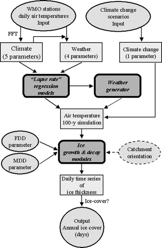
FIGURE 2. Southern Alps “lapse rate” regression relationships (weather-generator coefficients regressed on elevation). (a) Mean temperature (φ₀). (b) Phase of 1-yr cycle. (c) Second-order autoregression coefficient (φ₂). (d) Standard deviation of the daily temperature anomalies (σ)

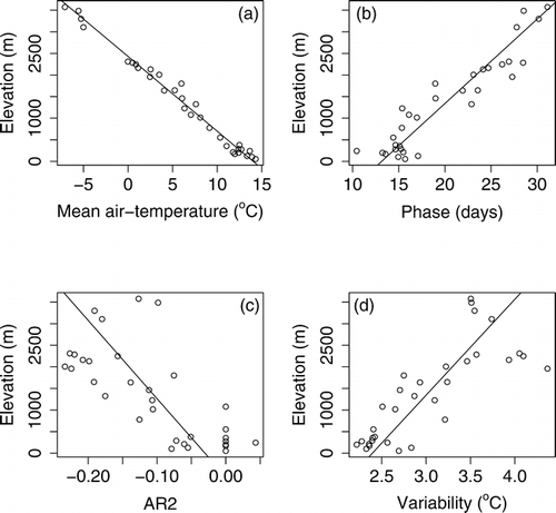
FIGURE 3. Scanning electron micrograph of diatoms from Lake Toskal, Finland (sample 25). This sample, from a depth of 25.5 cm below the lake floor, is typical of sediment from a remote alpine or sub-Arctic lake. The sample consists predominantly of well-preserved diatom valves and has an average (median) particle size of 15 μm

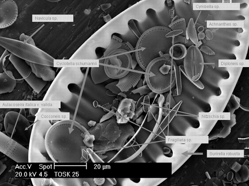
FIGURE 4. Simulations of ice-cover duration, at elevations between 0 and 4000 m in the Southern Alps, for eight climate-change scenarios (curves are drawn for scenarios at temperatures +6°C, +4.5°C, +3°C, +1.5°C, −1.5°C −3°C, −4.5°C, and −6°C different from the mean annual temperatures of the present day at a given elevation). Results are for a 100-yr-long simulation. The central (thicker) line depicts the present-day situation

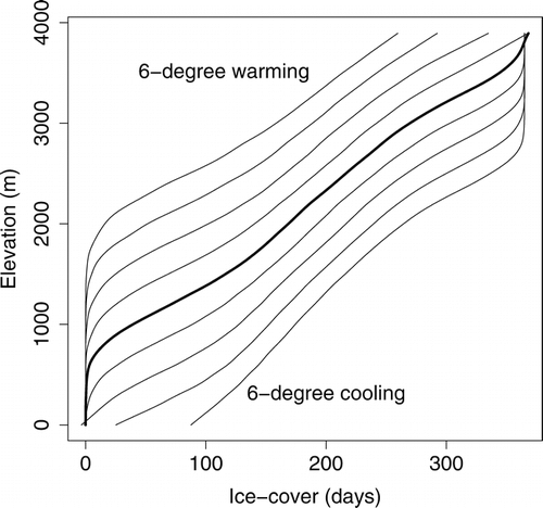
FIGURE 5. Change to ice-cover duration, at elevations between 0 and 4000 m in the Southern Alps, for the nine climate-change scenarios of Figure 4. (a) Modeled using a 100-yr-long full simulation (1-yr and 6-month cycles, plus weather). (b) Modeled using only climate (1-yr and 6-month cycles, no weather)

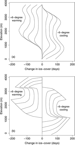
FIGURE 6. Number of diatom species vs. ice-cover duration. Relationship, optima, and tolerances. The optima plotted here are based on one PLS component

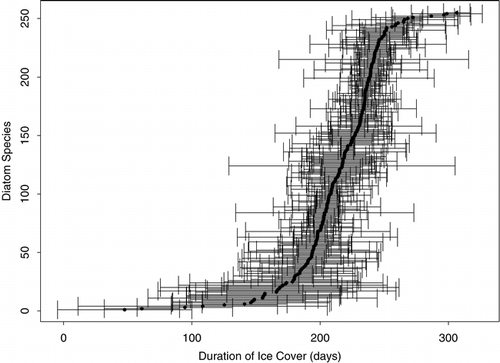
TABLE 1 Lapse-rate coefficients of weather generator for Southern Alps

TABLE 2 Pan-European data set (459 lakes, 252 taxa). For each variable, R ² is the coefficient of determination (range: 0 to +1); skill is a measure of the model's predictive ability (range: −∞ to +100%); root mean square error (RMSE) is the error associated with reconstructing the site environmental variables; and root mean square error of prediction (RMSEP) is the error associated with predicting the site environmental variables (in this case after jack-knifing)

TABLE 3 Northern Fennoscandia (151 lakes, 122 taxa). For each variable, R ², Skill, RMSE, and RMSEP are as in Table 2

Acknowledgments

We gratefully acknowledge NERC (Natural Environment Research Council) (GR9/04195), CHILL-10000, and EMERGE for financial support. Funds for the Abisko training set were provided through the Climate Impacts Research Centre (CIRC) within the Miljö och Rymdinstitutet (MRI). Climate data were obtained from the excellent CRU, NOAA, and NCDC databases. We thank S. Derrick for the diatom preparation and for the SEM photograph.

Notes

Revised ms submitted December 2004

References Cited

- Agusti-Panareda, A. and R. Thompson . 2002. Reconstructing air temperature at eleven remote alpine and arctic lakes in Europe from 1781 to 1997 AD. Journal of Paleolimnology 28:7–23.
- Akaike, H. 1974. A new look at the statistical model identification. IEEE Transactions on Automatic Control 19:716–723.
- Anderson, N. J. 2001. Diatoms, temperature and climatic change. European Journal of Phycology 35:307–314.
- Ansley, C. F. 1979. An algorithm for the exact likelihood of a mixed autoregressive-moving average process. Biometrika 66:59–65.
- Battarbee, R. W. , S. T. Patrick , B. Wathne , R. Psenner , and R. Mosello . 2002. Measuring and modelling the dynamic response of remote mountain lake ecosystems to environmental change (the MOLAR project). Verhandlungen der Internationalen Vereinigung für Theoretische und Angewandte Limnologie 27:3774–3779.
- Bigler, C. and R. I. Hall . 2002. Diatoms as indicators of climatic and limnological change in Swedish Lapland: A 100-lake calibration set and its validation for paleoecological reconstructions. Journal of Paleolimnology 27:97–115.
- Bigler, C. and R. I. Hall . 2003. Diatoms as quantitative indicators of July temperature: A validation attempt at century-scale with meteorological data from northern Sweden. Palaeogeography, Palaeoclimatology, Palaeoecology 189:147–160.
- Bilello, M. A. 1964. Method for predicting river and lake ice formation. Journal of Applied Meteorology 3:38–44.
- Birks, H. J B. 1995. Quantitative palaeoenvironmental reconstructions. In Maddy, D., Brew, J. S. (eds.), Statistical modelling of Quaternary science data. Cambridge: Quaternary Research Association, Technical Guide 5, 161–254.
- Birks, H. J B. 1998. Numerical tools in paleolimnology—Progress, potentialities, and problems. Journal of Paleolimnology 20:307–332.
- Bloomfield, P. 1976. Fourier analysis of time series: An introduction. New York: Wiley, 258 pp.
- Broecker, W. S. 2001. Was the Medieval Warm Period global?. Science 291:1497–1499.
- Burn, D. H. and A. Hag Elnur . 2002. Detection of hydrologic trends and variability. Journal of Hydrology 255:107–122.
- Cameron, N. G. , H. J B. Birks , V. J. Jones , F. Berge , J. Catalan , R. J. Flower , J. Garcia , B. Kawecka , K. A. Koinig , A. Marchetto , P. Sánchez-Castillo , R. Schmidt , M. Šiško , N. Solovieva , E. Štefková , and M. Toro . 1999. Surface-sediment and epilithic diatom pH calibration sets for remote European mountain lakes (AL:PE Project) and their comparison with the Surface Waters Acidification Programme (SWAP) calibration set. Journal of Paleolimnology 22:291–317.
- Cubasch, U. , G. A. Meehl , G. J. Boer , R. J. Stouffer , M. Dix , A. Noda , C. A. Senior , S. Raper , and K. S. Yap . 2001. Projections of future climate change. In Houghton, J. T., Ding, Y., Griggs, D. J., Noguer, M., van der Linden, P., Dai, X., Maskell, K., Johnson, C. I. (eds.), Climate change 2001: The scientific basis. Contribution of Working Group I to the Third Assessment Report of the Intergovernmental Panel on Climate Change. Cambridge: Cambridge University Press, 525–582.
- Deevey, E. S. 1969. Coaxing history to conduct experiments. BioScience 19:40–43.
- Gabriel, K. R. and J. Neumann . 1962. A Markov chain model for daily rainfall occurrence at Tel Aviv. Quarterly Journal of Royal Meteorological Society 88:90–95.
- Gates, P. and H. Tong . 1976. On Markov chain modelling to some weather data. Journal of Applied Meteorology 15:1145–1151.
- Giorgi, F. , M. R. Marinucci , and G. Visconti . 1992. A 2×CO2 climate change scenario over Europe generated using a limited area model in a general circulation model. II: Climate change scenario. Journal of Geophysical Research 97:10011–10028.
- Giorgi, F. , J. W. Hurrell , M. R. Marinucci , and M. Beniston . 1997. Elevation signal in surface climate change: A model study. Journal of Climate 10:288–296.
- Goutte, C. 1997. Note on free lunches and cross-validation. Neural Computation 9:1211–1215.
- Gyalistras, D. 2002. How uncertain are regional climate change scenarios? Examples for Europe and the Alps. In Gerstengarbe, F. W. (ed.), Angewandte Statistik—PIK-Weiterbildungsseminar 2000/2001: Potsdam, Germany: Potsdam Institute for Climate Impact Research, PIK Report 75, 85–93.
- Hulme, M. , D. Conway , P. D. Jones , E. M. Barrow , T. Jiang , and C. Turney . 1995. A 1961–90 climatology for Europe for climate change modelling and impacts applications. International Journal of Climatology 15:1333–1363.
- Hustedt, F. 1927–1966. Die Kieselalgen Deutschlands, Österreich und der Schweiz mit Berucksichtigung der ubrigen Lander Europas sowie der angrenzenden Meeresgebiete, Part I, II, III: Dr. L. Rabenhorst's Kryptogamen-Flora. Leipzig, Akademische Verlagsgesellschaft Geest und Portig K.-G., Volume 7, Part I, 1–920: Part II, 1–845: Part III, 1–816.
- Jones, P. D. and R. Thompson . 2003. Instrumental records. In Mackay, A. W., Battarbee, R. W., Birks, H. J. B., Oldfield, F. (eds.), Global change in the Holocene. London: Arnold, 140–158.
- Jones, V. J. and H. J B. Birks . 2004. Lake-sediment records of recent environmental change on Svalbard: Results of diatom analysis. Journal of Paleolimnology 31:445–466.
- Joynt, E. H. and A. P. Wolfe . 2001. Paleoenvironmental inference models from sediment diatom assemblages in Baffin Island lakes (Nunavut, Canada) and reconstruction of summer water temperature. Canadian Journal of Fisheries and Aquatic Sciences 58:1222–1243.
- Katz, R. W. 1977. Precipitation as a chain-dependent process. Journal of Applied Meteorology 16:671–676.
- Kettle, H. and R. Thompson . 2004. Statistical downscaling in European mountains: Verification of reconstructed air temperature. Climate Research 26:2 97–112.
- Kettle, H. , R. Thompson , J. Anderson , and D. M. Livingstone . 2004. Empirical modeling of summer lake surface water temperatures in southwest Greenland. Limnology and Oceanography 49:271–282.
- Kinderman, A. J. and J. F. Monahan . 1977. Computer generation of random variables using the ratio of uniform deviates. ACM Transactions on Mathematical Software 3:257–260.
- Kolbe, R. W. 1927. Zür Ökologie, Morphologie und Systematik der Brackwasser-Diatomeen. Pflanzenforschung, Heft 7: Jena: Verlag von Gustav Fischer, 143 pp. 3 Tfln.
- Korhola, A. , K. Vasko , H. T T. Toivonen , and H. Olander . 2002. Holocene temperature changes in northern Fennoscandia reconstructed from chironomids using Bayesian modelling. Quaternary Science Reviews 21:1841–1860:.
- Lorenz, E. N. 1956. Empirical orthogonal functions and statistical weather prediction. Cambridge, MA: Department of Meteorology, Massachusetts Institute of Technology, Statistical Forecast Project Report 1, Contract AF19(604)-1566, 49 pp.
- Lotter, A. F. , H. J B. Birks , W. Hofmann , and A. Marchetto . 1997. Modern diatom, cladocera, chironomid, and chrysophyte cyst assemblages as quantitative indicators for the reconstruction of past environmental conditions in the Alps: I. Climate. Journal of Paleolimnology 18:395–420.
- Magnuson, J. J. , D. M. Robertson , B. J. Benson , R. H. Wynne , D. M. Livingstone , T. Arai , R. A. Assel , R. G. Barry , V. Card , E. Kuusisto , N. G. Granin , T. D. Prowse , K. M. Stewart , and V. S. Vuglinski . 2000. Historical trends in lake and river ice cover in the Northern Hemisphere. Science 289:1743–1746.
- Miller, A. J. 1990. Subset selection in regression. London: Chapman and Hall, 229 pp.
- Pienitz, R. , J. P. Smol , and H. J B. Birks . 1995. Assessment of freshwater diatoms as quantitative indicators of past climatic change in the Yukon and Northwest Territories, Canada. Journal of Paleolimnology 13:21–49.
- Richardson, C. W. 1981. Stochastic simulation of daily precipitation, temperature, and solar radiation. Water Resources Research 17:182–190.
- Rosén, P. , R. I. Hall , T. Korsman , and I. Renberg . 2000. Diatom-transfer functions for quantifying past air temperature, pH and total organic carbon concentration from lakes in northern Sweden. Journal of Paleolimnology 24:109–123.
- Sarle, W. S. 1995. Stopped training and other remedies for overfitting. In Proceedings of the 27th Symposium on the Interface of Computing Science and Statistics, Pittsburgh, 27: 352–360. Retrieved from World Wide Web: ftp://ftp.sas.com/pub/neural/ .
- Seppä, H. , M. Nyman , A. Korhola , and J. Weckström . 2002. Changes of tree-lines and alpine vegetation in relation to post-glacial climate dynamics in northern Fennoscandia based on pollen and chironomid records. Journal of Quaternary Science 17:287–301.
- Sorvari, S. , M. Rautio , and A. Korhola . 2000. Seasonal dynamics of subarctic Lake Saanajärvi in Finnish Lapland. Verhandlungen der Internationalen Vereinigung für Theoretische und Angewandte Limnologie 27:507–512.
- Sorvari, S. , A. Korhola , and R. Thompson . 2002. Lake diatom response to recent arctic warming in Finnish Lapland. Global Change Biology 8:171–181.
- Stefan, H. G. and X. Fang . 1997. Simulated climate change effects on ice and snow covers on lakes in a temperate region. Cold Regions Science and Technology 25:137–52.
- ter Braak, C. J F. and S. Juggins . 1993. Weighted averaging partial least squares regression (WA-PLS): An improved method for reconstructing environmental variables from species assemblages. Hydrobiologia 269/270:485–502.
- Weckström, J. and A. Korhola . 2001. Patterns in the distribution, composition and diversity of diatom assemblages in relation to ecoclimatic factors in Arctic Lapland. Journal of Biogeography 28:31–45.
- Weckström, J. , A. Korhola , and T. Blom . 1997. Diatoms as quantitative indicators of pH and water temperature in subarctic Fennoscandian lakes. Hydrobiologia 347:171–184.
- Zhu, H. and R. Rohwer . 1996. No free lunch for cross-validation. Neural Computation 8:1421–1426.