Forecasting the seasonality and trend of pulmonary tuberculosis in Jiangsu Province of China using advanced statistical time-series analyses

Abstract

Objective

Forecasting the seasonality and trend of pulmonary tuberculosis is important for the rational allocation of health resources; however, this foresting is often hampered by inappropriate prediction methods. In this study, we performed validation research by comparing the accuracy of the autoregressive integrated moving average (ARIMA) model and the back-propagation neural network (BPNN) model in a southeastern province of China.

Methods

We applied the data from 462,214 notified pulmonary tuberculosis cases registered from January 2005 to December 2015 in Jiangsu Province to modulate and construct the ARIMA and BPNN models. Cases registered in 2016 were used to assess the prediction accuracy of the models. The root mean square error (RMSE), mean absolute percentage error (MAPE), mean absolute error (MAE) and mean error rate (MER) were used to evaluate the model fitting and forecasting effect.

Results

During 2005–2015, the annual pulmonary tuberculosis notification rate in Jiangsu Province was 56.35/100,000, ranging from 40.85/100,000 to 79.36/100,000. Through screening and comparison, the ARIMA (0, 1, 2) (0, 1, 1)₁₂ and BPNN (3-9-1) were defined as the optimal fitting models. In the fitting dataset, the RMSE, MAPE, MAE and MER were 0.3901, 6.0498, 0.2740 and 0.0608, respectively, for the ARIMA (0, 1, 2) (0, 1, 1)₁₂ model, 0.3236, 6.0113, 0.2508 and 0.0587, respectively, for the BPNN model. In the forecasting dataset, the RMSE, MAPE, MAE and MER were 0.1758, 4.6041, 0.1368 and 0.0444, respectively, for the ARIMA (0, 1, 2) (0, 1, 1)₁₂ model, and 0.1382, 3.2172, 0.1018 and 0.0330, respectively, for the BPNN model.

Conclusion

Both the ARIMA and BPNN models can be used to predict the seasonality and trend of pulmonary tuberculosis in the Chinese population, but the BPNN model shows better performance. Applying statistical techniques by considering local characteristics may enable more accurate mathematical modeling.

Keywords:

• ARIMA
• BPNN
• tuberculosis
• incidence
• forecasting

Introduction

Tuberculosis (TB) is a chronic infectious disease caused by Mycobacterium tuberculosis, with the most common form being pulmonary tuberculosis (PTB). Although the global TB incidence has declined by 1–2% per year,¹ it is still a major public health problem in many developing countries.^2,3 The WHO proposed an End TB Strategy in 2014, with the targets being to reduce TB deaths by 95% and to cut incident cases by 90% between 2015 and 2035.⁴ To achieve this ambitious goal, accurate prediction of disease trends, as well as related factors, is of great importance.^5,6

One of the commonly used prediction models is the autoregressive integrated moving average (ARIMA) model, which is a time series analysis tool proposed by George Box and Gwilym Jenkins in the 1970s.⁷ The ARIMA model regards the data sequence formed by the prediction object over time as a random sequence. This model is easy to construct, only requires intrinsic variables, and has relatively high prediction accuracy. The ARIMA model has been widely used in the prediction of such diseases as malaria,⁸ influenza,⁹ hemorrhagic fever¹⁰ or hand, foot and mouth disease.¹¹ Since the 1980s, the artificial neural network (ANN) model has been developed and rapidly applied as an effective tool in time series analysis and disease prediction. The ANN model can adjust its structure to adapt to the characteristics of samples, overcome the shortcomings of traditional parametric models that have high requirements on samples, and automatically recognize and learn the relationship between variables without any restrictions.^12–14 Therefore, this model has attracted more and more attention in the field of medicine and biology.^15–17 In 1986, the back-propagation neural network (BPNN) model was proposed by Rumelhant and Mc Clelland as one of the most commonly used ANNs.¹⁸ This model has been introduced into the dye and plastic industries, as well as dentistry. However, few studies are available on the ability of the improved BPNN model on PTB.^19–21

The ARIMA is a model that can capture the linear part of the incidence trend, while the BPNN model has a strong nonlinear fitting ability.^22,23 As the properties of the two models are distinct, they have differing abilities to predict disease trends. This study discusses the ARIMA and the BPNN in fitting and forecasting the incidence of PTB in Jiangsu Province, China. The DOTS (direct observed therapy, short course) strategy was introduced in China in the 1990s and is 100% available at the county level at present.²⁴ However, there are still great challenges facing TB control, particularly for the early detection and effective treatment of the disease. Based on surveillance data from 2005 to 2016, we performed validation research by comparing the fitting and forecasting performance of the ARIMA model and BPNN model with the aim of providing a valuable tool for the early warning of PTB outbreaks and epidemics.

Materials and methods

Study area and data collection

As a province located along the eastern coast of China, Jiangsu covers an area of 103.2 thousand square kilometers and contains 13 municipalities and 80 million permanent populations. All newly diagnosed TB cases are registered in an online Tuberculosis Management Information System (TBIMS), which is operated by the Center for Disease Control and Prevention (CDC) of China.²⁵ The TBIMS collects key information on TB cases notified in health facilities and exchanges data with the National Infectious Disease Reporting System. We extracted monthly data of PTB cases notified from January 2005 to December 2016 as the study subjects. Population data were obtained from the Jiangsu Provincial Statistical Yearbook. We used the notification rate from January 2005 to December 2015 as the model-construction dataset and notification rate from January 2016 to December 2016 as the validation dataset.

Construction of the ARIMA model

We construct the seasonal ARIMA model written as ARIMA (p, d, q) (P, D, Q)_s, where p, d and q stand for the autoregressive order, the number of nonseasonal differences and the moving average order, respectively, and P, D and Q stand for the seasonal autoregressive order, the number of seasonal differences and the seasonal moving average order, respectively. The s in the model represents the seasonal period length. In this study, we define the s as 12.⁹ The construction of the ARIMA model in this study contains four steps. First, we apply both nonseasonal difference and seasonal difference methods to stabilize the series, since the incidence series plot shows a declining trend and seasonal fluctuations. The series is considered to be stationary after difference according to the Augmented Dickey-Fuller (ADF) test. Second, we identify parameters (p, q, P and Q) to establish plausible models by referring to the autocorrelation function (ACF) and partial autocorrelation function (PACF) plots based on the stationary series. We first determine the seasonal part parameters (P and Q) and then the nonseasonal part parameters (p and q) for the ARIMA model. The model with the lowest corrected Akaike’s information criterion (AICc) and Bayesian information criterion (BIC) is defined as the optimal model. Third, we use the maximum likelihood method to estimate the parameters and the Ljung-Box test to examine the residuals of the optimal model. The residuals should be white noise, indicating that the model completely extracted information from the original data. Moreover, the ACF and PACF plots of the residuals should show no significant correlation.^26–28 Finally, the optimal model is applied to predict the PTB incidence.

Construction of the BPNN model

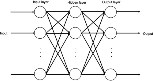
The BPNN is a typical multilayer feedforward neural network consisting of an input layer, hidden layer and output layer. Each layer is connected to another, but without interconnections between neurons in the same layer.¹² The basic algorithm of BPNN includes two processes: forward propagation of the signal and reverse propagation of the error. During the forward propagation step of the signal, the sample is input by the input layer, subjected to nonlinear processing at the hidden layer, and then passed to the output layer. The output value is compared to the expected value at the output layer. If the expected requirement is not met, the error needs to be propagated back. During the back-propagation step of the error, the output error is back transported layer by layer to the hidden layer and input layer. By adjusting the weight of each neuron in each hidden layer, the error is gradually reduced until the error between the actual output and the expected output meets the requirement of accuracy or reaches the maximum number of learning.²² The construction of the BPNN model generally includes six steps. First, we normalize the primary notification rate data and convert all values to intervals [0, 1] using the following formula: ${\mathrm{X}}^{\prime }=\frac{X-X_{min}}{X_{max}-X_{min}}$, where $\mathrm{X}$ is the original notification rate, $X_{max}$ is the maximum value of original notification rate, $X_{min}$ is the minimum value of original notification rate and ${\mathrm{X}}^{\prime }$ is the notification rate after conversion. Second, we determine a three-layer BPNN model with one input layer, one hidden layer and one output layer (Figure 1). We construct the BPNN model by dividing the data into a training set, testing set and validation set, according to the ratio of 7:1.5:1.5.¹⁴ Third, we preliminarily determine the number of neurons in the hidden layer using the empirical formula: $\mathrm{M}=\sqrt{\mathrm{n}+\mathrm{m}}+\mathrm{a}$, where M is the number of neurons in the hidden layer, n is the number of neurons in the input layer, m is the number of neurons in the output layer and a is a constant in the range of 1 to 10.¹⁸ Fourth, we set the target error of the training of BPNN as 0.001, the training steps as 1000, the transfer function of hidden layer as “tansig”, the transfer function of output layer as “purelin”, and the training function of network as “trainlm”. We construct BPNN models with different numbers of neurons in the hidden layer to train, test and validate each model using the training set, the testing set and the validation set, respectively. Fifth, we select the optimal model by comparing the mean squared error (MSE) values of the testing set of each model: $\mathrm{M}\mathrm{S}\mathrm{E}=\frac{1}{n}\sum _{i=1}^n{\left(X_i-{\hat{X}}_i\right)}^2$, where $X_i$ is the inverse normalized value of the output value of the testing sample i (forecasting incidence), ${\hat{X}}_i$ is the inverse normalized value of the expected output value of the testing sample i (actual incidence), and n is the number of testing samples. The model with the minimum MSE value is regarded as the optimal model.^22,29,30 Finally, the optimal BPNN model is applied to predict the PTB incidence.

Figure 1 Structure diagram of three-layer BPNN. BPNNs start as a network of nodes in three layers: the input, hidden and output layers. The input and output layers serve as nodes to buffer input and output for the model, respectively, and the hidden layer serves to provide a means for input relations to be represented in the output.

Evaluating the performance of models

The diagnostic statistics, including root mean square error (RMSE), mean absolute percentage error (MAPE), mean absolute error (MAE) and mean error rate (MER), are used to evaluate the fitting and forecasting performance of the two models in the study site: $\mathrm{R}\mathrm{M}\mathrm{S}\mathrm{E}=\sqrt{\frac{1}{n}\sum _{i=1}^n{\left(X_i-{\hat{X}}_i\right)}^2}$, $\mathrm{M}\mathrm{A}\mathrm{P}\mathrm{E}=\frac{1}{n}\sum _{i=1}^n\frac{\left|X_i-{\hat{X}}_i\right|\ast 100}{X_i}$, $\mathrm{M}\mathrm{A}\mathrm{E}=\frac{1}{n}\sum _{i=1}^n\left|X_i-{\hat{X}}_i\right|$, and $\mathrm{M}\mathrm{E}\mathrm{R}=\frac{\frac{1}{n}{\sum }_{i=1}^n\left|X_i-{\hat{X}}_i\right|}{\overline{X_i}}$, where $X_i$ is the actual notification rate at time i, ${\hat{X}}_i$ is the fitting or forecasting notification rate at time i, $\overline{X_i}$ is the mean of the actual notification rate, and n is the number of samples.

Statistical software

We used the packages including “forecast”, “ggplot2” and “tseries” of R3.6.0 (https://www.r-project.org/) to construct the ARIMA model and the MATLAB R2017a (MathWorks, Massachusetts, USA) to construct the BPNN model.

Results

ARIMA model

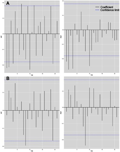
During 2005–2015, 462,214 PTB cases were newly notified in Jiangsu Province with an annual notification rate of 56.35/100,000, ranging from 40.85/100,000 to 79.36/100,000. The monthly notification series plot showed a declining trend and seasonal fluctuations (Figure 2). The peak incidence mainly occurred in March, April and May, and the trough was more common in November and December. We made one nonseasonal difference (d=1) and one seasonal difference (D=1) to stabilize the incidence series. The ADF test remained significant (P<0.001), indicating a stationary series. The ACF and PACF plots of the stationary notification series are shown in Figure 3A. For the seasonal part of the ARIMA model, there was a significant spike at lag 12 in the ACF plot and the PACF plot, respectively, but without a significant spike at lag 24 in the ACF plot or the PACF plot (P=0 and Q=1). For the nonseasonal part of the ARIMA model, we initially considered eight possibilities: p=0 and q=1; p=0 and q=2; p=1 and q=0; p=1 and q=1; p=1 and q=2; p=2 and q=0; p=2 and q=1; p=2 and q=2, since the ACF and PACF plots did not show an obvious pattern. The AICc and BIC values of eight plausible ARIMA models are listed in Table S1. We selected ARIMA (0,1,2) (0,1,1)₁₂ as the optimal model because it had the minimum AICc and BIC values. The parameter estimation of this model is shown in Table S2. All parameters of this model were significant (P<0.001). The Ljung-Box test confirmed that the residuals of this model were white noise (P>0.05). As shown in Figure 3B, the ACF and PACF plots of residuals also proved to be white noise, since their correlation coefficients did not show significant correlation. Although the autocorrelation coefficient and the partial correlation coefficient were beyond the confidence limit at lag 10, it could be considered accidental because it only occurred once in a total of 24 lags. Then, we applied the ARIMA (0,1,2) (0,1,1)₁₂ model to predict the monthly PTB notification rate in 2016. The predictive value and the actual data are listed in Table 1. The ARIMA model had a relatively high prediction accuracy, where the relative errors of predictive value in each month (except for September and October) were less than 10%.

Table 1 Predicted monthly notification rate of pulmonary tuberculosis in 2016 using the ARIMA and BPNN model

Month	Actual rate (1/100,000)	ARIMA model		BPNN model
		Predicted rate (1/100,000)	Relative error (%)	Predicted rate (1/100,000)	Relative error (%)
January	3.2053	3.4841	8.6993	3.4040	6.2003
February	3.3202	3.1820	4.1611	3.0431	8.3446
March	3.6519	3.8289	4.8465	3.8584	5.6543
April	3.3473	3.4243	2.3015	3.3539	0.1983
May	3.4079	3.3945	0.3942	3.3395	2.0081
June	3.2169	3.2337	0.5228	3.1029	3.5433
July	3.0516	3.1349	2.7280	3.0476	0.1327
August	3.2272	3.3069	2.4693	3.2627	1.0997
September	2.7780	3.1142	12.1030	2.9947	7.8013
October	2.5973	2.9138	12.1875	2.6476	1.9383
November	2.6102	2.6428	1.2502	2.6086	0.0600
December	2.5766	2.4842	3.5863	2.6185	1.6260

Figure 2 Monthly notification rate of pulmonary tuberculosis from January 2005 to December 2015 in Jiangsu, China.

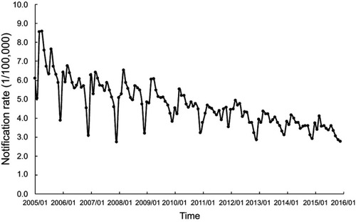
Figure 3 ACF and PACF plots. The autocorrelation function (ACF) and partial autocorrelation function (PACF) plots of pulmonary tuberculosis notification series after one nonseasonal and one seasonal difference (A). The ACF and PACF plots of residuals of the ARIMA (0,1,2) (0,1,1)₁₂ model (B).

BPNN model

We used the notification rate in the same month of the past three years as the input data and the notification rate in the same month of the next year as the output data. The notification data from January 2005 to December 2015 in the study setting could form 96 samples. We defined n=3 and m=1. Thus, the number of neurons in the hidden layer ranged from 3 to 12. We constructed 10 different BPNN models, with the number of neurons in the hidden layer ranging from 3 to 12, and compared the MSE value of the testing set in each model (Table S3). We finally chose the 3-9-1 BPNN model because it had the minimum MSE value of 0.00190, containing 9 neurons in the hidden layer. We applied the optimal BPNN model to predict the monthly PTB notification rate in 2016 using the notification rate of corresponding months between 2013 and 2015 as input values. The predictive values are shown in Table 1. The results indicated that the BPNN model performed better than the ARIMA model, since the relative errors of all months were less than 10% and the relative errors of eight months were less than 5%.

Comparison of the ARIMA model and BPNN model

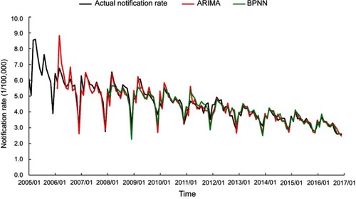
We compared the performance of the ARIMA model and BPNN model in fitting and forecasting the PTB notification rate (Table 2). Although the BPNN model was slightly inferior to the ARIMA model in forecasting PTB in a few months in 2016, in general, the BPNN model was superior to ARIMA model either in fitting or forecasting performance, which was confirmed by Figure 4. Moreover, Figure 4 also showed that the BPNN model performed better in fitting or forecasting the peak and trough notification rate.

Table 2 Comparison of the fitting and forecasting performance of the two models

Evaluation index	Fitting performance		Forecasting performance
	ARIMA	BPNN	ARIMA	BPNN
RMSE	0.3901	0.3236	0.1758	0.1382
MAPE	6.0498	6.0113	4.6041	3.2172
MAE	0.2740	0.2508	0.1368	0.1018
MER	0.0608	0.0587	0.0444	0.0330

Abbreviations: RMSE, root mean square error; MAPE, mean absolute percentage error; MAE, mean absolute error; MER, mean error rate.

Figure 4 Fitting and forecasting curves of the ARIMA and BPNN models compared with the actual notification rate of pulmonary tuberculosis.

Furthermore, we applied the two models to predict the notification rate of PTB by gender (male and female) and age (<65 and ≥65 years old) and then compared the predictive accuracy of the two models. The results are listed in Table S4 and S5. Stratification analysis suggested that the BPNN was superior to the ARIMA model in predicting PTB in different groups of people, especially among the elderly.

Discussion

Although the TB incidence in China is considered lower than the global average, due to the large population base, China is still ranked as one of the top 30 high burden countries.³¹ To achieve the goal of “End TB”, accurate prediction of TB incidence is of great practical significance for effective TB prevention and control. According to the predicted data, we can carry out targeted prevention and control measures and allocate health resources effectively. To date, different models have been developed.³² To the best of our knowledge, this study is the first to compare the application of the ARIMA model and BPNN model in predicting PTB in the southeastern part of China. Our results suggested that the BPNN model was superior to the ARIMA model to fit or forecast the PTB notification rate in the study setting, either in the entire population or in specific groups with different genders or ages.

The PTB incidence in Jiangsu Province has shown an obvious declining trend and significant seasonal variation. The peak occurs mostly in March, April and May, while the trough is more common in November and December, which is similar to the time distribution at the national level of China.³³ Seasonal fluctuations may be related to such factors as sunshine hours, vitamin D levels, and temperature.^34–37 This fluctuation may also be attributed to delays in the monitoring system, which needs to be confirmed in further studies.

The ARIMA model assumes that there is a certain relationship between the future state of the target object and the historical data of the past and the present.³⁸ According to the seasonal fluctuations of the target sequence, the ARIMA model can be divided into a seasonal model or a nonseasonal model. This model overcomes the limitation of the requirement for a prior assumption about the development mode of the time series. The process of identification, estimation, and diagnosis is repeated until the optimized model is obtained.³⁹ The ARIMA model is widely used in many types of time series analysis and is by far the most versatile time series prediction method. Anwar et al used the ARIMA (4,1,1) (1,0,1)₁₂ model to predict future malaria incidence in Afghanistan.⁸ Li et al used the ARIMA (0,1,1) (2,1,0)₁₂ model to forecast the incidence of hemorrhagic fever with renal syndrome in Hebei Province, China.¹⁰ Mahmood et al used the ARIMA (0,1,1) (0,1,1)₁₂ model to predict the incidence of smear-positive TB cases in Iran.⁴⁰ However, the ARIMA model is only suitable for a short-term prediction and can only capture the linear relationship in the incidence trend. As the occurrence of TB is affected by many known and unknown factors, the incidence trend tends to exhibit nonlinear characteristics, which can not be effectively solved through the ARIMA model.

Compared with other traditional models, the BPNN model has several advantages. First, BPNN can adjust its structure to adapt to the characteristics of samples, overcome the shortcomings of traditional parametric models that have high requirements on the distribution of samples, and automatically recognize and learn the relationship between variables without any restrictions. Second, due to the strong fault tolerance, this model will have less excessive impact on the entire network when there is a local error. Third, the BPNN model can handle almost any nonlinear function, avoiding the complicated parameter estimation process. Fourth, the construction of BPNN has a standard process, with intuitive results.^18,22,30 However, the determination of structure is a major difficulty in the BPNN model construction process, especially for defining the number of neurons in the hidden layer. At present, there is no fully generic modeling guidance. When the number of neurons in the hidden layer is too small, the established model will be too simple to fully extract the inherent laws of the data, resulting in underfitting rsults. When the number of neurons is too large, the established network structure may be too complicated, leading to the overfitting results. This effect will reduce the generalization ability of the model and influence its application.²² Considering that the BPNN model initially used a random function to define weights and thresholds and that the results of each training step in the same model were different, in the actual model construction process, we used the loop control statement to train the model repeatedly and picked out the best one for subsequent predictive analysis.

To minimize the possibility of underfitting or overfitting, we took the following measures in the process of constructing models. For the ARIMA model, we used the Ljung-Box test to help us estimate whether the model fully exploited the original data. If the residuals were shown to be white noise, we concluded that there might be a low possibility of underfitting in the model. To avoid overfitting as much as possible, we used the AICc and BIC to select the optimal model from alternative plausible models. The model with the lowest value of AICc and BIC was considered because it had the least parameters when fitting data. For the BPNN model, we divided the samples into a training set, testing set and validation set and compared the MSE values to minimize the possibility of underfitting. To avoid the overfitting problem as much as possible, we used a relatively large sample size of 96 and set the training target error and the training steps at 0.001 and 1000, respectively.

Conclusion

Both ARIMA and BPNN models can be used to predict the incidence trend of PTB in the Chinese population, but the BPNN model shows better performance. There are no fully generic models used for the prediction of diseases across different areas. Applying statistical techniques by considering local characteristics may allow for more accurate mathematical modeling.

Ethics statement

This study was approved by the Ethics Committee of Nanjing Medical University. Personal information of patients did not appear in this study.

Availability of data and material

All data generated or analyzed during this study are included in this published article.

Author contributions

All authors contributed to data analysis, drafting or revising the article, gave final approval of the version to be published, and agree to be accountable for all aspects of the work.

Acknowledgments

The study was supported by the National Key R&D Program of China (2017YFC0907000), National Natural Science Foundation of China (81473027), National Thirteenth Five-year Mega-Scientific Projects of Infectious Diseases of China (2018ZX10103002-001-006, 2018ZX10103002-003-003), and Priority Academic Program Development of Jiangsu Higher Education Institutions (PAPD). The funders had no role in the study design, data collection and analysis, decision to publish, or preparation of the manuscript.

Supplementary materials

Table S1 AICc and BIC values of plausible ARIMA models

Model	AICc	BIC
ARIMA (0,1,1) (0,1,1)12	141.40	149.53
ARIMA (0,1,2) (0,1,1)12	125.38	136.15
ARIMA (1,1,0) (0,1,1)12	148.69	156.82
ARIMA (1,1,1) (0,1,1)12	127.68	138.45
ARIMA (1,1,2) (0,1,1)12	127.18	140.55
ARIMA (2,1,0) (0,1,1)12	139.89	150.65
ARIMA (2,1,1) (0,1,1)12	129.18	142.54
ARIMA (2,1,2) (0,1,1)12	127.98	143.91

Abbreviations: AICc, corrected Akaike’s information criterion; BIC, Bayesian information criterion.

Table S2 Estimation of parameters of the ARIMA (0,1,2) (0,1,1)₁₂ model

Model parameter	Coefficient	Standard error	t	P
Moving average, lag 1	−0.3928	0.0955	−4.1131	<0.001
Moving average, lag 2	−0.4763	0.1022	−4.6605	<0.001
Seasonal moving average, lag 1	−0.3708	0.0967	−3.8345	<0.001

Table S3 MSE value of the testing set for each BPNN model

BPNN model	MSE value
3-3-1	0.00213
3-4-1	0.00224
3-5-1	0.00240
3-6-1	0.00195
3-7-1	0.00194
3-8-1	0.00201
3-9-1	0.00190
3-10-1	0.00219
3-11-1	0.00196
3-12-1	0.00198

Abbreviation: MSE, mean squared error.

Table S4 Results of the ARIMA model and BPNN model in predicting the notification rate of pulmonary tuberculosis in 2016 stratified by gender and age (1/100,000)

Month	Gender						Age
	Male			Female			<65 years old			≥65 years old
	Actual	ARIMA predicted	BPNN predicted	Actual	ARIMA predicted	BPNN predicted	Actual	ARIMA predicted	BPNN predicted	Actual	ARIMA predicted	BPNN predicted
January	4.7549	5.1572	4.9022	1.7002	1.9573	1.8783	2.6438	2.8080	2.7215	6.9226	8.6812	7.6708
February	4.9125	4.7192	4.4675	1.7939	1.8723	1.7956	2.6797	2.5983	2.5012	7.6002	8.0333	7.1867
March	5.4284	5.7392	5.4041	1.9970	2.0679	2.0668	3.1211	3.1675	3.0040	7.4811	9.3395	8.2260
April	4.9786	5.1159	4.8499	1.8147	1.8921	1.9112	2.8637	2.8784	2.8409	6.7944	7.8263	7.3190
May	5.0243	5.0620	4.7315	1.9345	1.9415	1.9443	2.9610	2.8876	2.8779	6.7852	7.8386	7.1387
June	4.8337	4.7884	4.6277	1.7366	1.8575	1.8331	2.7425	2.7463	2.6466	6.7211	7.2426	6.8969
July	4.4474	4.7160	4.4694	1.8121	1.8753	1.8776	2.7066	2.6751	2.7029	5.8329	7.4751	6.6067
August	4.7905	4.9499	4.6786	1.9215	1.9975	1.9816	2.8368	2.7528	2.7830	6.6570	8.3445	7.3572
September	4.0281	4.6531	4.4504	1.7705	1.9200	1.9130	2.4897	2.6069	2.3979	5.5033	7.4646	6.8874
October	3.9036	4.4690	4.2955	1.5856	1.8136	1.7813	2.2982	2.5474	2.4319	5.5674	7.1963	6.7429
November	3.9696	4.0522	4.0310	1.5413	1.6487	1.5798	2.3416	2.3916	2.3577	5.3934	5.9772	5.7561
December	4.0306	4.1180	4.1145	1.5622	1.4737	1.4187	2.3790	2.2608	2.2731	5.4483	6.4144	6.1477

Table S5 Comparison of the ARIMA model and the BPNN model in predicting the notification rate of pulmonary tuberculosis stratified by gender and age

Evaluation index	Gender				Age
	Male		Female		<65 years old		≥65 years old
	ARIMA	BPNN	ARIMA	BPNN	ARIMA	BPNN	ARIMA	BPNN
RMSE	0.3082	0.2452	0.1296	0.1095	0.1086	0.0954	1.3693	0.7485
MAPE	5.5154	4.3549	6.4602	5.3549	3.3873	3.0944	20.1145	10.9470
MAE	0.2429	0.1948	0.1103	0.0915	0.0862	0.0817	1.2606	0.6714
MER	0.0529	0.0424	0.0632	0.0519	0.0323	0.0306	0.1972	0.1050

Abbreviations: RMSE, root mean square error; MAPE, mean absolute percentage error; MAE, mean absolute error; MER, mean error rate.

Disclosure

The authors report no conflicts of interest in this work.

References

- Raviglione M, Marais B, Floyd K, et al. Scaling up interventions to achieve global tuberculosis control: progress and new developments. Lancet. 2012;379(9829):1902–1913. doi:10.1016/S0140-6736(12)60727-222608339
- Sgaragli G, Frosini M. Human tuberculosis I. Epidemiology, diagnosis and pathogenetic mechanisms. Curr Med Chem. 2016;23(25):2836–2873.27281297
- Bele S, Jiang W, Lu H, et al. Population aging and migrant workers: bottlenecks in tuberculosis control in rural China. PLoS One. 2014;9(2):e88290. doi:10.1371/journal.pone.008829024498440
- WHO. The End TB Strategy. 2014 Available from: https://www.who.int/tb/post2015_strategy/en/. Accessed 1218, 2018.
- Heesterbeek H, Anderson RM, Andreasen V, et al. Modeling infectious disease dynamics in the complex landscape of global health. Science. 2015;347(6227):aaa4339. doi:10.1126/science.aaa433925766240
- Arora G, Misra R, Sajid A. Model systems for pulmonary infectious diseases: paradigms of anthrax and tuberculosis. Curr Top Med Chem. 2017;17(18):2077–2099. doi:10.2174/156802661766617013011132428137237
- Lin Y, Chen M, Chen G, Wu X, Lin T. Application of an autoregressive integrated moving average model for predicting injury mortality in Xiamen, China. BMJ Open. 2015;5(12):e008491. doi:10.1136/bmjopen-2015-008491
- Anwar MY, Lewnard JA, Parikh S, Pitzer VE. Time series analysis of malaria in Afghanistan: using ARIMA models to predict future trends in incidence. Malar J. 2016;15(1):566.27876041
- He Z, Tao H. Epidemiology and ARIMA model of positive-rate of influenza viruses among children in Wuhan, China: a nine-year retrospective study. Int J Infect Dis. 2018;74:61–70.29990540
- Li Q, Guo NN, Han ZY, et al. Application of an autoregressive integrated moving average model for predicting the incidence of hemorrhagic fever with renal syndrome. Am J Trop Med Hyg. 2012;87(2):364–370. doi:10.4269/ajtmh.2012.11-047222855772
- Liu L, Luan RS, Yin F, Zhu XP, Lu Q. Predicting the incidence of hand, foot and mouth disease in Sichuan province, China using the ARIMA model. Epidemiol Infect. 2016;144(1):144–151. doi:10.1017/S095026881500114426027606
- Peng JC, Ran ZH, Shen J. Seasonal variation in onset and relapse of IBD and a model to predict the frequency of onset, relapse, and severity of IBD based on artificial neural network. Int J Colorectal Dis. 2015;30(9):1267–1273. doi:10.1007/s00384-015-2250-625976931
- Wang D, Wang Q, Shan F, Liu B, Lu C. Identification of the risk for liver fibrosis on CHB patients using an artificial neural network based on routine and serum markers. BMC Infect Dis. 2010;10:251. doi:10.1186/1471-2334-10-25120735842
- Hale AT, Stonko DP, Lim J, Guillamondegui OD, Shannon CN, Patel MB. Using an artificial neural network to predict traumatic brain injury. J Neurosurg Pediatr. 2018;23(2):219–226. doi:10.3171/2018.8.PEDS1837030485240
- Wang CH, Mo LR, Lin RC, Kuo JJ, Chang KK, Wu JJ. Artificial neural network model is superior to logistic regression model in predicting treatment outcomes of interferon-based combination therapy in patients with chronic hepatitis C. Intervirology. 2008;51(1):14–20. doi:10.1159/00011879118309244
- Baxt WG. Application of artificial neural networks to clinical medicine. Lancet. 1995;346(8983):1135–1138. doi:10.1016/s0140-6736(95)91804-37475607
- Khan MT, Kaushik AC, Ji L, Malik SI, Ali S, Wei DQ. Artificial neural networks for prediction of tuberculosis disease. Front Microbiol. 2019;10:395. doi:10.3389/fmicb.2019.0039530886608
- Wang J, Wang F, Liu Y, et al. Multiple linear regression and artificial neural network to predict blood glucose in overweight patients. Exp Clin Endocrinol Diabetes. 2016;124(1):34–38. doi:10.1055/s-0035-156517526797861
- Attallah O, Ma X. Bayesian neural network approach for determining the risk of re-intervention after endovascular aortic aneurysm repair. Proc Inst Mech Eng H. 2014;228(9):857–866. doi:10.1177/095441191454998025212212
- Bibi H, Nutman A, Shoseyov D, et al. Prediction of emergency department visits for respiratory symptoms using an artificial neural network. Chest. 2002;122(5):1627–1632. doi:10.1378/chest.122.5.162712426263
- Chang CL, Li MY. Predictions of diffuse pollution by the HSPF model and the back-propagation neural network model. Water Environ Res. 2017;89(8):732–738. doi:10.2175/106143017X1490296825466528743327
- Guan P, Huang DS, Zhou BS. Forecasting model for the incidence of hepatitis A based on artificial neural network. World J Gastroenterol. 2004;10(24):3579–3582. doi:10.3748/wjg.v10.i24.357915534910
- Yan W, Xu Y, Yang X, Zhou Y. A hybrid model for short-term bacillary dysentery prediction in Yichang City, China. Jpn J Infect Dis. 2010;63(4):264–270.20657066
- Shao Y, Yang D, Xu W, et al. Epidemiology of anti-tuberculosis drug resistance in a Chinese population: current situation and challenges ahead. BMC Public Health. 2011;11:110. doi:10.1186/1471-2458-11-11021324205
- Huang F, Cheng S, Du X, et al. Electronic recording and reporting system for tuberculosis in China: experience and opportunities. J Am Med Inform Assoc. 2014;21(5):938–941. doi:10.1136/amiajnl-2013-00200124326537
- Liu Q, Liu X, Jiang B, Yang W. Forecasting incidence of hemorrhagic fever with renal syndrome in China using ARIMA model. BMC Infect Dis. 2011;11:218. doi:10.1186/1471-2334-11-20821838933
- Wang T, Liu J, Zhou Y, et al. Prevalence of hemorrhagic fever with renal syndrome in Yiyuan County, China, 2005-2014. BMC Infect Dis. 2016;16:69. doi:10.1186/s12879-016-1987-z26852019
- Zhou L, Zhao P, Wu D, Cheng C, Huang H. Time series model for forecasting the number of new admission inpatients. BMC Med Inform Decis Mak. 2018;18(1):39. doi:10.1186/s12911-018-0683-x29907102
- Chen S, Zhou S, Zhang J, Yin FF, Marks LB, Das SK. A neural network model to predict lung radiation-induced pneumonitis. Med Phys. 2007;34(9):3420–3427. doi:10.1118/1.275960117926943
- Li H, Luo M, Zheng J, et al. An artificial neural network prediction model of congenital heart disease based on risk factors: a hospital-based case-control study. Medicine (Baltimore). 2017;96(6):e6090. doi:10.1097/MD.000000000000609028178169
- WHO. Global tuberculosis report 2018 Available from: https://www.who.int/tb/publications/global_report/en/. Accessed 1218, 2018.
- Li Z, Wang Z, Song H, et al. Application of a hybrid model in predicting the incidence of tuberculosis in a Chinese population. Infect Drug Resist. 2019;12:1011–1020. doi:10.2147/IDR.S19041831118707
- Wang H, Tian CW, Wang WM, Luo XM. Time-series analysis of tuberculosis from 2005 to 2017 in China. Epidemiol Infect. 2018;146(8):935–939. doi:10.1017/S095026881800111529708082
- Li XX, Wang LX, Zhang H, et al. Seasonal variations in notification of active tuberculosis cases in China, 2005-2012. PLoS One. 2013;8(7):e68102. doi:10.1371/journal.pone.006810223874512
- Koh GC, Hawthorne G, Turner AM, Kunst H, Dedicoat M. Tuberculosis incidence correlates with sunshine: an ecological 28-year time series study. PLoS One. 2013;8(3):e57752. doi:10.1371/journal.pone.005775223483924
- Thorpe LE, Frieden TR, Laserson KF, Wells C, Khatri GR. Seasonality of tuberculosis in India: is it real and what does it tell us? Lancet. 2004;364(9445):1613–1614. doi:10.1016/S0140-6736(04)17316-915519633
- Wang M, Kong W, He B, et al. Vitamin D and the promoter methylation of its metabolic pathway genes in association with the risk and prognosis of tuberculosis. Clin Epigenetics. 2018;10(1):118. doi:10.1186/s13148-018-0552-630208925
- Brockwell PJ, Davis RA. Time series: theory and methods. Technometrics. 1989;31(1):121. doi:10.1080/00401706.1989.10488491
- Box GEP, Jenkins GM, Reinsel GC. Time series analysis: forecasting and control. Rev. ed J Time. 1976;31(4):238–242.
- MOOSAZADEH M, KHANJANI N, NASEHI M, BAHRAMPOUR A. Predicting the incidence of smear positive tuberculosis cases in iran using time series analysis. Iran J Public Health. 2015;44(11):1526–1534.26744711