MODENA: a multi-objective RNA inverse folding

Abstract

Artificially synthesized RNA molecules have recently come under study since such molecules have a potential for creating a variety of novel functional molecules. When designing artificial RNA sequences, secondary structure should be taken into account since functions of noncoding RNAs strongly depend on their structure. RNA inverse folding is a methodology for computationally exploring the RNA sequences folding into a user-given target structure. In the present study, we developed a multi-objective genetic algorithm, MODENA (Multi-Objective DEsign of Nucleic Acids), for RNA inverse folding. MODENA explores the approximate set of weak Pareto optimal solutions in the objective function space of 2 objective functions, a structure stability score and structure similarity score. MODENA can simultaneously design multiple different RNA sequences at 1 run, whose lowest free energies range from a very stable value to a higher value near those of natural counterparts. MODENA and previous RNA inverse folding programs were benchmarked with 29 target structures taken from the Rfam database, and we found that MODENA can successfully design 23 RNA sequences folding into the target structures; this result is better than those of the other benchmarked RNA inverse folding programs. The multi-objective genetic algorithm gives a useful framework for a functional biomolecular design. Executable files of MODENA can be obtained at http://rna.eit.hirosaki-u.ac.jp/modena/.

Keywords:

• multi-objective genetic algorithm
• secondary structure
• RNA sequence design
• Rfam

Introduction

To date, a variety of cellular functions of noncoding RNAs (ncRNAs) has been elucidated using experimental and computational methodologies. Since RNA secondary structures play important roles in their functions, various RNA folding algorithms (eg, those based on minimization of free-energy [MFE],^1,2 formal grammar,^3,4 and maximum expected accuracy⁵) have been developed to analyze RNA sequences. Recently, RNA secondary structure has become an important notion not only to unveil the cellular functions of natural ncRNAs but also to create artificial RNA molecules which have a desired function (such as artificial ribozymes,⁶ artificial miRNAs,⁷ and RNA nanostructures^8,9). In such artificial applications of RNA sequence, we have to design an RNA sequence that folds into a desired structure (target structure) to realize a desired function. This ‘RNA sequence design’ problem can be defined as an inverse problem of the RNA folding. Since no RNA inverse folding algorithm that can find all RNA sequences folding to a desired structure is yet known, heuristic algorithms, RNAinverse,¹⁰ RNA-SSD¹¹ and INFO-RNA,¹² have been proposed to solve approximately the RNA inverse folding problem. RNA inverse is a pioneering RNA inverse folding algorithm which uses a divide-and-conquer type strategy, where the inverse folding proceeds from sub-sequences to a whole sequence, and an adaptive walk is used to iteratively improve the designed sequence. RNA-SSD also uses a divide-and-conquer type strategy (hierarchical decomposition of the target secondary structure) and a stochastic local search¹³ to improve the RNA sequence given by a sophisticated sequence initialization procedure. INFO-RNA is well characterized by its strong sequence initialization procedure; in this initialization, a dynamic programming algorithm is employed to find the RNA sequence which has the lowest free energy in all compatible RNA sequences, where the free energies are calculated by assuming all compatible RNA sequences are folded into the target structure (the RNA sequences that can form a structure strictly the same as that of a given target structure are called ‘compatible sequences’,¹⁰ where the target structure does not need to be the optimal structure of each sequence). This initialization is followed by a stochastic local search¹³ which iteratively examines neighboring RNA sequences in the RNA sequence space. This local search is done according to the order determined based on the free energy differences between the current and neighboring sequences.

Motivation

Although the previous RNA inverse folding algorithms have shown high performance in various benchmarks, they have the following drawbacks. i) First, these algorithms tend to output the RNA sequences with a narrow range of free energies. This could be due to the search algorithms and objective function (OF) used in the previous algorithms. The previous algorithms adopt local search algorithms to minimize the structure distance between designed and target structures, and do not use a free energy as an OF. As a result, they tend to output the RNA sequences near to the initial RNA sequence. For example, INFO-RNA tends to output an RNA sequence much more stable than the corresponding natural ncRNAs,¹⁴ and this is likely to be due to the initial guess of INFO-RNA, which already has a very low free energy. If possible, selecting the stability of the designed RNA sequence from a wider range would be more favorable, since the stability can affect the function of the designed RNA sequence. ii) Second, the direct problem solver (ie, an RNA folding program) of the previous methods is fixed. In RNA inverse folding, a direct problem solver is iteratively used to predict the structure of the designed sequence, which is necessary to compare the structure of the designed sequence with the target structure; eg, RNAinverse, RNA-SSD and INFO-RNA use a fold function of Vienna RNA Package² as a direct problem solver. Although it may be theoretically possible to change the direct problem solver in the previous methods to the other one, such an implementation is currently not available. Since more accurate RNA folding algorithms based on new paradigms, such as Sfold¹⁵ and CentroidFold,⁵ have been proposed, an RNA inverse folding algorithm should also has an option to use a new RNA folding program as a direct problem solver.

To address the drawback i) mentioned above, we have to consider 2 objective functions simultaneously, a stability measure (such as a free energy) and a structure similarity measure (such as the structure distance between the designed and target structures), during the optimization. This indicates that RNA inverse folding can be formulated as a multi-objective problem, whereas the previous algorithms have adopted a structure distance alone as an objective function to be optimized. Multi-objective optimization (MOO)¹⁶ is a methodology for solving multi-objective problems. So far, many applications of MOO in bioinformatics have been reported.^17,18 On the basis of MOO, we can simultaneously optimize multiple objective functions without assigning a relative weight to each objective function. To solve the MOO problems, multi-objective genetic algorithms (MOGAs),¹⁶ eg, nondominated sorting genetic algorithm 2 (NSGA2),^16,19 have been developed and widely used. In the present paper, we show that MOGA gives a useful framework for biomolecular sequence design, and our new RNA inverse folding algorithm, called MODENA (Multi-Objective DEsign of Nucleic Acids), can improve the 2 drawbacks pointed out for the previous RNA inverse folding algorithms.

Material and methods

In RNA inverse folding, we explore an RNA sequence space to find the RNA sequences that fold into a user-given target structure, where ‘a sequence folds into a structure’ means that the structure is the optimal structure (eg, the lowest free energy structure or the centroid structure) of the sequence. The sequence length N is determined by the length of the inputted target structure. A point of the RNA sequence space for the sequences with a length of N is denoted by S = s₁··s_i··s_N (1 ≤ i ≤ N), where s_i ∈ {A, C, G, U} for all i; an A, C, G and U indicates an adenine, cytosine, guanine and uracil, respectively. An RNA structure is composed of loop nucleotides and base pairs, where a base pair (i, j) indicates formation of the hydrogen bonds between nucleotide positions i and j (where 1 ≤ i < j ≤ N and usually |i – j| > 3). Moreover, the RNA structure can be represented by using a connection information c_i, where if position i forms a base pair with position j, c_i = j; when position i is a loop nucleotide, c_i = 0.

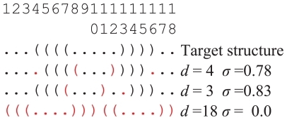
To explore the RNA sequence which folds into the desired target structure and has the lowest possible free energy, we have to take into account 2 objective functions simultaneously: a measure for structure stability (such as the free energy E computed by a direct problem solver) and a measure for structure similarity (eg, the structure distance d between the structure predicted for the designed RNA sequence and the target structure given by a user). In the present study, we use a structure stability score ɛ and a structure similarity score σ as the objective functions. The ɛ and σ are defined as ɛ = –E and σ = (N – d)/N, respectively, where E and N are the lowest free energy of the designed sequence and the total number of nucleotides, respectively; a structure distance d is the number of the nucleotide positions whose structure in the designed sequence is different from that in the target structure (Figure 1). A larger value of the ɛ corresponds to more stable structure. The similarity score σ scale ranges from 0.0 to 1.0 and a similarity score of 1.0 indicates a perfect consensus between 2 structures.

Figure 1 Examples of a structure distance d and similarity score σ between a target structure (denoted as ‘target structure’) and 3 structures of designed sequences. Nucleotide positions whose structure in the designed sequence is different from that in the target structure are represented in red. The structure shown at the bottom has a σ = 0.0, ie, the target structure and the structure shown at the bottom are completely different.

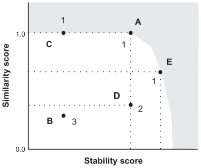
In the present paper, we introduce MOO to take the 2 objective functions into account in the RNA inverse folding. In MOO,¹⁶ we evaluate solutions by using a dominance, which is defined between 2 solutions. Let us consider exploring the solutions that maximize all objective functions. Solution A is said to dominate solution B if both of the following 2 conditions are satisfied: i) f_i^A ≥ f_i^B (∀i ∈1 … M), where f_i^A and f_i^B are the i-th objective functions of solutions A and B, respectively, and M is the number of objective functions; ii) f_i^A ≠ f_i^B (∃i ∈1 … M). In addition, solution A is said to strongly dominate solution B when f_i^A > f_i^B (∀i ∈1 … M). A Pareto optimal solution is a solution that is not dominated by any other solution, and a solution not strongly dominated by any other solution is called a weak Pareto optimal solution. In accordance with the definitions, 2 solutions with exactly the same values of objective functions are neither dominated nor strongly dominated each other. The definitions of the terminology (eg, dominance) written in italic in this paragraph are taken from Deb.¹⁶ A schematic illustration of a dominance relationship in RNA inverse folding is shown in Figure 2.

Figure 2 An example of a dominance relationship in the RNA inverse folding problem. Stability and similarity scores are used as objective functions. Each solid circle indicates a solution in the objective function space. In this figure, solutions A and E dominate solutions B and D; solution A also dominates solution C. Since solution C has a similarity score the same as that of solution A, solution A does not strongly dominate solution C. In this figure, a gray region schematically indicates the region where no solution exists; hence solutions A and E are Pareto optimal solutions. Since solution A is the Pareto optimal solution with a similarity score of 1.0, solution A has the highest stability score in all RNA sequences folding into a target structure. Solution C is not a Pareto optimal solution, but is included in weak Pareto optimal solutions. The integers assigned to each solution are the dominance ranks calculated for the 5 solutions, where the dominance ranks are calculated based on strong dominance.

Multi-objective genetic algorithm

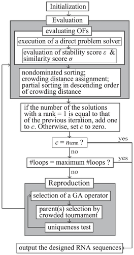
To obtain an approximate set of weak Pareto optimal solutions for RNA inverse folding, we developed an RNA inverse folding algorithm, MODENA, on the basis of NSGA2,^16,19 which is one of the standard MOGAs. A flowchart of MODENA is shown in Figure 3, where initialization, evaluation and reproduction procedures are used in accordance with the standard procedures of genetic algorithm (GA); GA is a population-based metaheuristics for a search and combinatorial optimization. ²⁰ In the initialization step, initial N_p solutions are generated in a random manner, where N_p is a GA population size. In MODENA, an RNA nucleotide sequence is used as a solution, and duplication of identical RNA sequences in one population is prohibited throughout a MODENA run. In the evaluation step, a direct problem solver is invoked to assign stability and similarity scores to each solution. After the evaluation step, reproduction procedures generate child solutions by applying mutations and a crossover to a parent population. The iteration between the evaluation and reproduction procedures stops when one of the following conditions is satisfied: i) a GA iteration number reaches a given maximum number of iterations; ii) the number of non-strongly dominated solutions in a GA population does not change during continuous n_term iterations. In the present study, n_term = 30 was used. Details of the initialization, evaluation and reproduction procedures are described below.

Figure 3 Flowchart of MODENA algorithm.

Abbreviations: GA, genetic algorithm; OF, objective function.

Initialization

In this step, we generate an initial population of N_p RNA sequences in a random manner. To generate the i-th individual of the initial population (1 ≤ i ≤ N_p), first, we define a probability p_AG = (i – 1.0)/(N_p – 1.0). Then we scan the nucleotide positions of i-th solution to assign a nucleotide as follows: if the position is a loop position in the target structure, we assign an adenine to the position with a probability of p_AG + (1.0 – p_AG) × 0.25, otherwise a cytosine, guanine, or uracil is assigned to the position with an equal probability; if the position has a base pair, a guanine is assigned to the position with a probability of p_AG + (1.0 – p_AG) × 0.25, otherwise an adenine, cytosine, or uracil is assigned to the position with an equal probability.

In addition to the procedure mentioned above, we perform 2 procedures for the initialization of the i-th individual. The first one is a ‘random change from a guanine to cytosine’. In this procedure, a guanine assigned to each nucleotide position is randomly changed to a cytosine with a probability of 0.5. This procedure is introduced to shuffle a guanine and cytosine in the base paired positions without changing a base pair type (a G:C and C:G are the same base pair type). The second one is a ‘propagation procedure’ where the generated RNA sequence is scanned from the 5′ end to the 3′ end, and if we find a position i which forms a base pair with a position j (where i < j), a nucleotide compensatory to the nucleotide at the position i is assigned to the position j, where only canonical A:U and G:C pairs are used (eg, if G is found at position i, C is assigned to position j; a G:U pair is not used). This procedure guarantees that the randomly generated RNA sequence is a compatible RNA sequence for the target structure.

By using the procedures mentioned above with a high p_AG, we can obtain an RNA sequence that has GC-rich base paired positions and A-rich loop positions, and we can expect that such an RNA sequence has a high stability score. In contrast, when we use a low p_AG, we can obtain an RNA sequence with a lower stability score. By using the formula p_AG = (i – 1.0)/(N_p – 1.0) for the i-th solution, we can fill the initial population with RNA sequences that have diverse values of stability scores, and such a set of RNA sequences can give a good initial guess for obtaining an approximate set of weak Pareto optimal solutions.

Evaluation

In the evaluation step, the stability score ɛ and similarity score σ for each solution are evaluated. To calculate the 2 objective functions, we have to run a direct problem solver for each solution since both the lowest free energy (which is needed to obtain the stability score) and a structure (which is needed to calculate the structure similarity with the target structure) are computed by the direct problem solver. As a direct problem solver, we can utilize RNAfold² and CentroidFold⁵ in MODENA. A default direct problem solver is RNAfold. These direct problem solvers can be specified through an option of MODENA.

After evaluating the objective functions, in accordance with NSGA2,^16,19 MODENA assigns a dominance rank to each solution and determines the N_p parent solutions for the next GA generation as follows:

Step 1 We set R = (N_p parent solutions) + (N_p child solutions). It is noted that, at the first GA iteration, the child population is a null; ie, R = (N_p parent solutions) at the first GA iteration.

Step 2 A dominance rank is assigned to each solution in R. We use the O(MN_p²) nondominated sorting of the original NAGA2,¹⁶ where M is the number of objective functions.

Step 3 The solutions in R are sorted in ascending order of dominance rank.

Step 4 If both the N_p-th solution and the (N_p + 1)-th solution in R share a dominance rank of i, sorting in descending order of crowding distance¹⁶ is performed only for the solutions with a dominance rank of i; this procedure is called a ‘niching’. We use the top N_p solutions in R as the parent solutions at the next GA generation. Step 4 is not used at the first GA iteration since (N_p + 1)-th solution does not exist.

Reproduction

In the reproduction step of MODENA, in accordance with NSGA2,^16,19 we generate N_p child solutions from the parent N_p solutions. The child solutions are generated with randomly invoked GA operators. After selection of the GA operator, a parent solution is selected using crowded tournament selection,¹⁶ where a mutation and crossover operator needs 1 and 2 parent solutions, respectively. In the MODENA algorithm, we use 1 crossover operator (structural n-point crossover) and 2 mutation operators (point accepted mutation and error diagnosis mutation). The 3 GA operators are invoked with an equal probability, ie, 1/3.

Structural n-point crossover is performed with a crossover parameter n_c and a randomly determined x₀ (= 0 or 1) as follows:

Step 1 Set l = 0 and set x_i = x₀ for all i (1 ≤ i ≤ N; N is a sequence length). Randomly select a base pair (i, j) (1 ≤ i < j ≤ N).

Step 2 If x_k (i ≤ k ≤ j) is 0, change x_k to 1, otherwise change x_k to 0 for all k; then increment l by 1.

Step 3 If l < n_c and ‘the number of the base pairs whose upstream nucleotide position m satisfies i < m (where m < N)’ is larger than or equal to 1, randomly select a base pair (i^new, j^new), where i < i^new < j^new ≤ N; then we set i = i^new and j = j^new, and move to Step 2; otherwise we go to Step 4.

Step 4 Generate a child solution according to x_i for all i (1 ≤ i ≤ N); if x_i = 0, copy the value of a nucleotide s_i^A in parent A to the corresponding nucleotide s_i^child of the child solution; if x_i = 1, the value of a nucleotide s_i^B in parent B is copied to s_i^child.

It is noted that we consider only the target structure and do not use a predicted structure in structural n-point crossover. The algorithm of structural n-point crossover is illustrated in Figure 4(a). In this study, we use n_c = 1 (a user can change this value with a command line option). As can be seen from the figure, structural n-point crossover splices the subsequences of 2 parent RNA sequences in such a way that the 2 nucleotides of each base pair are copied from 1 parent RNA sequence. By using the structural n-point crossover, we can crossover the parent RNA sequences without destroying the compensatory relationships in each parent RNA sequence.

Figure 4 Examples of the genetic algorithm operators used in the MODENA algorithm. a) Structural n-point crossover: parent A and parent B are randomly divided into subsequences (denoted in red and blue) in accordance with the target structure, where base pairs in each parent solution are preserved in each set of the subsequences. A child solution is generated by concatenating the subsequences selected from parent A (denoted in red) and those selected from parent B (denoted in blue). b) Point accepted mutation: randomly selected positions of the child solution are mutated. In this example, mutated positions are indicated in red. c) Error diagnosis mutation: examples corresponding to the rules (i), (ii) and (iii) are denoted in red, blue and green, respectively.

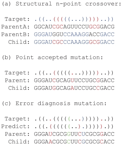
Point accepted mutation copies the parent sequence to the child sequence, and then scans the child sequence from the 5′ end in order to randomly change each nucleotide with a probability of p_M. If the position of the changed nucleotide forms a base pair with the other position k (1 ≤ k ≤ N) in the target structure, a nucleotide compensatory to the changed nucleotide is assigned to the position k, where an A:U or G:C base pair is used (Figure 4(b)).

In error diagnosis mutation operator, first we copy the nucleotide s_i^parent and connection information c_i^parent of a parent solution to the s_i^child and c_i^child of a child solution for all i (1 ≤ i ≤ N), respectively; here we copy the c_i^parent, which is assigned to the parent solution by a direct problem solver, to the child solution. Then, we scan the c_i^child (1 ≤ i ≤ N) of the child solution from the 5′ end. If we find a nucleotide position i which has a structure different from the corresponding one of the target structure (ie, when c_i^target ≠ c_i^child), a s_i^child is modified (and s _j^child, where 1 ≤ j ≤ N, is also modified if position i forms a base pair with position j in the target structure) in accordance with the following 3 rules:

1. when position i forms a base pair with position j in the predicted structure (ie, c_i^child = j, 1 ≤ i ≤ N, 1 ≤ j ≤ N) whereas position i has a loop nucleotide in the target structure (c_i^target = 0), we change a nucleotide s_i^child in accordance with the value of s _j^child; when s _j^child is an adenine, we set a cytosine or guanine to s_i^child ; if s _j^child is a cytosine, we set an adenine or uracil; if s _j^child is a guanine or uracil, we set an adenine or cytosine, respectively; these operations prevent a nondesired base pair formation when the child RNA sequence is folded by a direct problem solver.

2. when position i does not form a base pair in the predicted structure (c_i^child = 0) while the corresponding position in the target structure forms a base pair with position j (c_i^target = j), we set a C:G or G:C pair to a s_i^child:s_j^child pair.

3. if position i forms a base pair with position k in the predicted structure (c_i^target = k, 1 ≤ k ≤ N) whereas position i forms a base pair with position j (≠ k) in the target structure (c_i^target = j, 1 ≤ j ≤ N), we change the nucleotide s_i^child in accordance with the value of s_k^child; when s_k^child is an adenine, we set a cytosine or guanine to s_i^child; if s_k^child is a cytosine, we set an adenine or uracil; if s_k^child is a guanine or uracil, we set an adenine or cytosine, respectively; then a nucleotide compensatory to that of position i is assigned to s _j^child, where A:U or G:C base pairs are used.

An example of error diagnosis mutation is shown in Figure 4(c). It is noted that the operations by the rules (i)–(iii) are not independent of each other; during the scan from the 5′-end, an operation by a rule may overwrite the previous change made by another rule.

Datasets for the performance evaluation

We evaluated the performance of MODENA and other RNA inverse folding programs with the dataset taken from the seed alignments of Rfam 9.0.²¹ To evaluate the RNA design performance for RNA secondary structures, we extracted the annotated structures from 29 Rfam entries (from RF00001 to RF00030 except for RF00023), where each Rfam entry corresponds to an RNA family. RF00023 (Rfam ID:tmRNA) was not used since it has too many pseudoknots. In each Rfam entry, we selected the longest RNA sequence and extracted its annotated structure, and we used the extracted structure as the target structure of the Rfam entry. If pseudoknot base pairs are included in the extracted structure, pseudoknot base pairs were deleted from the extracted structure before the performance evaluation. As a result, we obtained 29 target secondary structures. Hereafter, we refer to this dataset as the Rfam dataset.

Results and discussion

Since MODENA is a ‘population-based’ algorithm based on GA, multiple solutions can be obtained at 1 run. In the present study, we use a GA population size N_p = 50 to evaluate the performance of MODENA. MODENA with this setting outputs at most 50 successfully designed RNA sequences at one run; we refer to the designed RNA sequence which has a similarity score of 1.0 as a ‘successfully designed RNA sequence’, and we refer to a run which outputs the successfully designed RNA sequence as a ‘successful run’.¹² A GA population size = 100 was also used in order to compare the results obtained with population sizes of 50 and 100. Throughout the present paper, we use a maximum GA iteration number equal to the population size (eg, we use a maximum iteration number = 50 when using a population size = 50). Performance comparison between MODENA and previous methods is not straightforward, since the previous methods are ‘nonpopulation-based’ algorithms, which output one solution at 1 run. To compare the performance of MODENA with those of nonpopulation-based algorithms (INFO-RNA 2.1 and RNAinverse of Vienna RNA Package 1.8.3), we performed 50 independent runs for each target structure when evaluating the nonpopulation-based methods. Independent multiple runs of a nonpopulation-based method can give multiple solutions different from each other, since the nonpopulation-based methods used in our performance comparison are stochastic algorithms.

Comparison of computational times of MODENA and the previous nonpopulation-based algorithms is also not straightforward. When we performed 50 independent runs of each nonpopulation-based algorithm for a target structure, we calculated ‘the expected time E_t required for finding a solution’, which was used in the previous studies.^11,12 The E_t is defined as follows:

$E_{\text{t}}=E_{\text{s}}+\left(\frac{1}{f_{\text{s}}}-1\right)E_{\text{u}},$(1)

where E_s is the average time of successful runs, E_u is the average time of unsuccessful runs, and f_s is a rate of successful runs (f_s = the number of successful runs divided by the total number of independent runs). The E_t gives an expected computational time for obtaining a successfully designed RNA sequence. When there is no successful run (ie, f_s = 0), the E_t and the computational time of MODENA are denoted as ‘−’ in our results. We discuss the computational speed of MODENA and other methods by comparing the computational time of 1 MODENA run and the E_t of other methods.

An approximate set of weak Pareto optimal solutions

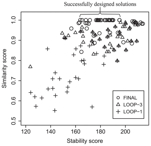
Figure 5 shows an example of how the solutions computed by MODENA evolve to the successfully designed RNA sequences. In the figure, we plot the solution distributions of the initial, third and final populations obtained in the GA iterations. In the initial distribution of this example, there are no successfully designed RNA sequences, ie, no solution has a similarity score of 1.0. These rather randomly distributed initial solutions successfully evolved to an approximate set of weak Pareto optimal solutions after 50 GA iterations, where 23 solutions with a wide range of stability scores were successfully designed. Moreover, we observed a fast convergence in this example; we obtained a solution distribution almost similar to that of the final population even at the tenth GA iteration (data not shown).

Figure 5 Example plots in an objective function space for the solutions obtained by MODENA. An RNA inverse folding result for a target structure (a structure of a rRNA predicted by RNAfold; GenBank accession number of the rRNA:AF107506) is shown. In this figure, the solution distribution of the initial genetic algoritham iteration (denoted by LOOP-1), that of the third iteration (LOOP-3) and the final one (FINAL) are shown. Successfully designed RNA sequences (ie, they have a similarity score of 1.0) are indicated as ‘successfully designed solutions’.

The results for the Rfam dataset

The performance evaluation results for the Rfam dataset are summarized in Table 1, where RNAfold was used as a direct problem solver of MODENA. In this table, the results for INFO-RNA and RNAinverse are also shown for the performance comparison. In the target structures taken from the annotations of the 29 RNA families in Rfam, MODENA successfully designed RNA sequences for 23 RNA families. This result is better than those obtained by INFO-RNA and RNAinverse, by which the RNA sequences of 17 and 13 RNA families were successfully designed, respectively. The free energy distributions for the successfully designed RNA sequences are shown in Figures 6, 7 and 8, where the results for the RNA families successfully designed by all methods (MODENA, INFO-RNA and RNAinverse) are represented. As can be seen from the figures, the RNA sequences designed by MODENA have much wider free energy ranges compared with those of INFO-RNA and RNAinverse. There are 2 possible reasons for this result. The first is the local search nature of INFO-RNA and RNAinverse. Since INFO-RNA and RNAinverse explore the region near to the initial RNA sequences, the initial guess can strongly affect the final RNA sequence. Interestingly, RNAinverse and INFO-RNA consistently outputs high free energy solutions and low free energy solutions, respectively, in our results. These results clearly correspond to the sequence initialization algorithms of the methods; RNAinverse uses a purely random compatible sequence as an initial sequence, while IFNO-RNA generates an initial sequence with a very low free energy by a dynamic programming. The second is the MOGA used in MODENA. MODENA is developed based on NSGA2; NAGA2 takes niching into account in the optimization procedure, which encourages the solutions in a population to be diverse in the objective function space. As a result, the approximate set of weak Pareto optimal solutions computed by MODENA tends to expand not only to a high stability score side but to a low stability score side. This leads to a wider free energy range of the RNA sequences designed by MODENA.

Figure 6 Free energy distributions of the successfully designed RNA sequences for a part of the Rfam dataset. The RNA family name and the accession number in Rfam are indicated at the top of the figure. The distributions for RNAinverse, INFO-RNA, and MODENA are shown by a boxplot. In the figure, the free energy of the natural RNA sequence corresponding to the target structure is also plotted as a ‘natural’, where the free energy was obtained by folding the RNA sequence with RNAfold.

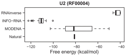
Figure 7 Free energy distributions of the successfully designed RNA sequences for a part of the Rfam dataset (continued from Figure 6).

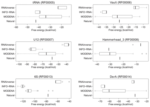
Figure 8 Free energy distributions of the successfully designed RNA sequences for a part of the Rfam dataset (continued from Figures 6 and 7).

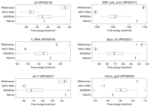
Table 1 The results for the Rfam dataset

Rfam AC	Rfam ID	MODENA			INFO-RNA		RNAinverse
		l (nt)	succ.	t (s)	succ.	Et (s)	succ.	Et (s)
RF00001	5S_rRNA	117	6/50	15.4	47/50	0.192	0/50	–
RF00002	5_8S_rRNA	151	20/50	17.2	0/50	–	0/50	–
RF00003	U1	161	22/50	23.8	0/50	–	0/50	–
RF00004	U2	193	34/50	23.8	24/50	8.531	5/50	142.418
RF00005	tRNA	74	33/50	4.4	50/50	0.021	39/50	0.117
RF00006	Vault	89	37/50	5.3	47/50	0.071	6/50	11.077
RF00007	U12	154	34/50	19.3	38/50	0.864	5/50	62.743
RF00008	Hammerhead_3	54	26/50	2.7	50/50	0.007	50/50	0.008
RF00009	RNaseP_nuc	348	29/50	106.6	0/50	–	0/50	–
RF00010	RNaseP_bact_a	357	0/50	–	0/50	–	0/50	–
RF00011	RNaseP_bact_b	382	0/50	–	0/50	–	0/50	–
RF00012	U3	215	27/50	30.1	0/50	–	0/50	–
RF00013	6S	185	12/50	23.2	22/50	10.779	7/50	73.390
RF00014	DsrA	87	33/50	6.5	50/50	0.021	50/50	0.019
RF00015	U4	140	38/50	11.7	23/50	5.473	2/50	284.150
RF00016	SNORD14	129	0/50	–	0/50	–	0/50	–
RF00017	SRP_euk_arch	301	28/50	99.0	43/50	3.167	8/50	155.517
RF00018	CsrB	360	24/50	139.3	0/50	–	0/50	–
RF00019	Y_RNA	83	32/50	5.7	50/50	0.024	33/50	0.215
RF00020	U5	119	0/50	–	0/50	–	0/50	–
RF00021	Spot_42	118	37/50	11.4	49/50	0.069	48/50	0.125
RF00022	GcvB	148	38/50	14.0	9/50	23.131	0/50	–
RF00024	Telomerase-vert	451	0/50	–	0/50	–	0/50	–
RF00025	Telomerase-cil	210	33/50	25.9	1/50	676.599	0/50	–
RF00026	U6	102	38/50	5.6	3/50	58.354	0/50	–
RF00027	let-7	79	32/50	7.3	50/50	0.035	47/50	0.094
RF00028	Intron_gpI	344	0/50	–	0/50	–	0/50	–
RF00029	Intron_gpII	73	37/50	3.8	41/50	0.024	8/50	1.140
RF00030	RNase_MRP	340	22/50	92.3	0/30	–	0/50	–

Notes: The evaluation results for the Rfam dataset. An ‘l’ column is the length (= number of nucleotides) of the target structure, a ‘succ.’ column represents the success rate, and t is computational time in seconds. In the results of MODENA, a success rate x/y means that we obtained x successfully designed sequences when we used a genetic algoritham population size of y. In the cases of INFO-RNA and RNAinverse, a success rate x/y means that x sequences were successfully designed when y independent runs were performed. E_t indicates the expected time required for finding a successfully designed sequence. Computational times were measured on a Core2Duo PC (2.8 GHz; a 2 Gbyte memory; CentOS 5.5).

Abbreviation: AC, accession number.

In almost all RNA families included in Figures 6, 7 and 8, the free energies of the natural RNA sequences corresponding to the target structures are located within the free energy range of MODENA, whereas the energy ranges of RNAinverse and INFO-RNA do not include the energies of the natural ones in almost all RNA families of Figures 6, 7 and 8.

To test the initial random number dependence of MODENA, we performed an additional 3 independent runs for the Rfam dataset with different initial random numbers. As a result, we found that the random number dependence of MODENA is very small, where only 1 run for RF00003 in an additional runs failed and the other RNA families, which were successfully designed in Table 1, were successfully designed in the additional 3 runs. It is noteworthy that we obtained 1 successful design of RF00028 in an additional run whereas design of this RNA family failed in Table 1.

As can be seen from Table 1, INFO-RNA is much faster than MODENA in many cases. Computational times of MODENA and RNAinverse are comparable.

To test the performance of the MODENA invoked with an option of a non-MFE direct problem solver (CentroidFold),⁵ we performed the RNA inverse folding with the Rfam dataset, where a population size of 50 was used. As a result, we successfully designed RNA sequences for 20 RNA families out of the 29 RNA families of the Rfam dataset. Since this result is slightly worse than that obtained with the MFE direct problem solver (RNAfold), we performed larger calculations with the CentroidFold direct problem solver on the failed 9 target structures of the Rfam dataset, where we set both a GA population size and maximum iteration number to 100. These larger calculations improved the results, where two out of the nine target structures were successfully designed. These results imply that RNA inverse folding with a non-MFE direct problem solver is more difficult than that with a MFE direct problem solver.

Why we explore weak Pareto optimal solutions

In the Pareto optimal solutions for the RNA inverse folding problem, where the stability score and similarity score are used as objective functions, there exists only 1 solution (eg, solution A in Figure 2) with a similarity score of 1.0 which folds into the target structure; this is because the other solutions (eg, solution C in Figure 2) with a similarity score of 1.0 (and a lower stability score) are dominated by the single Pareto optimal solution with a similarity score of 1.0. This indicates that the stability score of the Pareto optimal solution with a similarity score = 1.0 is highest in the stability scores of all RNA sequences folding into the target structure. The other solutions (eg, solution E in Figure 2) in the Pareto optimal solutions have a similarity score σ < 1.0.

It is noted that even when we successfully find the single solution which has a similarity score of 1.0 and the best stability score in all RNA sequences folding into the target structure, our search does not finish. This is because the other solutions (eg, solution C in Figure 2) with a lower stability score and a similarity score of 1.0 usually exist and they are also acceptable as solutions of RNA inverse folding. Since not only very stable RNA structures but also those with a lower stability can be candidates for artificial functional RNA sequences, it is important to develop a methodology that can design the RNA sequences with a wide range of free energies. To obtain a set of the RNA sequences that fold into the target structure and have a wide range of stability score, we can utilize weak Pareto optimal solutions. In weak Pareto optimal solutions of the RNA inverse folding problem, multiple solutions are allowed to have a similarity score of 1.0 in contrast to the case of the Pareto optimal solutions, where only 1 solution is allowed to have a similarity score of 1.0 (in Figure 2, solutions A and C are weak Pareto optimal solutions). Thus, weak Pareto optimal solutions can give more a comprehensive solution set for RNA inverse folding. Since it is difficult to obtain the complete set of weak Pareto optimal solutions, we explored the approximate set of weak Pareto optimal solutions in the RNA inverse problem by using a framework of MOGA.

Conclusions

We have developed a new RNA inverse folding algorithm, MODENA, on the basis of MOGA. We have evaluated MODENA with the dataset taken from Rfam, and found that our program can successfully design 23 RNA sequences out of the 29 target secondary structures. This result is better than those of the previous RNA inverse folding algorithms, INFO-RNA and RNAinverse, which successfully designed 17 and 13 RNA sequences, respectively. MODENA can not only design the RNA sequences successfully but also output multiple solutions with a wide range of free energies at 1 run. In addition, we showed that MODENA can design RNA sequences on the basis of a non-MFE-based state-of-the-art RNA folding program.

The advantage of MODENA is the ability to produce successfully designed multiple RNA sequences with a wide range of free energies. Currently, this function has not been realized by the other RNA inverse folding algorithms. This function enables us to select not only a very stable RNA secondary structure but also an RNA sequence whose secondary structure has a free energy similar to that of natural counterparts.

It is noted that the RNA sequence designed by an RNA inverse folding program is a ‘predicted candidate’; ie, there is no guarantee that the designed RNA sequence folds to the structure exactly same as that of the specified structure in vivo. For this reason, an experimenter will have to assess a number of computationally designed RNA sequences before obtaining an RNA sequence that has a desired function.

For example, riboswitches⁶ are interesting targets of the RNA sequence design. Riboswitches show a conformational change when they work; if the designed riboswitch sequence has too stable a structure, the riboswitch may not work correctly since a too stable structure can disturb the conformational change necessary to function as a riboswitch. In such a case, selecting a designed RNA sequence whose free energy is not too low but near that of natural counterparts will become important. Moreover, in other ncRNAs, if the cleavage of the RNA strands of the ncRNA is necessary to work as a functional RNA, a similar situation can occur.

A slow computational speed is the drawback of MODENA. Since MODENA executes a direct problem solver many times (if we use a population size of 50 and a maximum GA iteration number of 50, the direct problem solver is called at most 2500 times), the computational time of MODENA strongly depends on the speed of the direct problem solver. MODENA is based on GA, and GA can be accelerated by using a parallel computation; a parallel computation is a promising way to hasten MODENA and such an implementation is currently in progress.

The objective functions of MODENA still have a degree of freedom. In the current version of MODENA, the probability of the lowest energy structure of the designed RNA sequence is not used in the objective functions.¹⁰ By using the probability as the stability score instead of –E, we can explore the RNA sequence whose lowest energy structure has the largest probability. Implementation of this direction is not difficult, and we will include such a function also in the next versions.

It is noteworthy that the framework of the MOO allows us to optimize not only a system with 2 objective functions but also that with more objective functions. This means that the MODENA algorithm can potentially be extended to various different purposes. We believe that the MODENA algorithm gives a useful framework for the inverse folding of a great variety of biomolecules.

Acknowledgments

This work was partially supported by KAKENHI (22700304).

Disclosure

The author reports no conflicts of interest.