Review of the mathematical functions used to model the temperature dependence of electrical and thermal conductivities of biological tissue in radiofrequency ablation

Abstract

Purpose: Although theoretical modelling is widely used to study different aspects of radiofrequency ablation (RFA), its utility is directly related to its realism. An important factor in this realism is the use of mathematical functions to model the temperature dependence of thermal (k) and electrical (σ) conductivities of tissue. Our aim was to review the piecewise mathematical functions most commonly used for modelling the temperature dependence of k and σ in RFA computational modelling.

Materials and methods: We built a hepatic RFA theoretical model of a cooled electrode and compared lesion dimensions and impedance evolution with combinations of mathematical functions proposed in previous studies. We employed the thermal damage contour D63 to compute the lesion dimension contour, which corresponds to Ω = 1, Ω being local thermal damage assessed by the Arrhenius damage model.

Results: The results were very similar in all cases in terms of impedance evolution and lesion size after 6 min of ablation. Although the relative differences between cases in terms of time to first roll-off (abrupt increase in impedance) were as much as 12%, the maximum relative differences in terms of the short lesion (transverse) diameter were below 3.5%.

Conclusions: The findings suggest that the different methods of modelling temperature dependence of k and σ reported in the literature do not significantly affect the computed lesion diameter.

• Electrical conductivity
• radiofrequency ablation
• thermal conductivity
• theoretical modelling
• tissue characteristics

Introduction

High temperature ablative techniques use radiofrequency (RF), laser, microwave, or ultrasound energy to heat biological tissues to over 50 °C. In particular, RF ablation (RFA), is a minimally invasive technique that uses electrical currents (≈500 kHz) to heat the target biological tissue. It has been increasingly used in recent years for the treatment of cancer in the liver [1], kidney [2], bone [3], breast [4], prostate [5] and lung [6].

Clinical trials, experimental studies (in vivo or ex vivo), phantom-based models and theoretical modelling have been used to study different aspects of RFA. Although theoretical models can provide information about the biophysics of RFA quickly and cheaply, it is important for them to be as realistic as possible [7]. The mathematical functions used to model the temperature dependence of tissue characteristics are one of the most important factors in achieving realism. Electrical (σ) and thermal conductivity (k) in particular show significantly varying values due to the phenomena associated with the high temperatures reached during RFA, such as water vaporisation at temperatures near 100 °C and the subsequent sudden rise in impedance, which impedes the delivery of RF power, hence limiting the lesion size.

Previous theoretical studies have assessed the impact of absolute values of σ and k on lesion geometry [8–10]. However, we are now interested in reviewing the mathematical functions employed to model the temperature dependence of σ and k, since previous computer modelling studies used different approaches. As far as we know, no previous studies have critically reviewed and assessed the effect of these mathematical functions on the computed lesion size. Our aim was to assess how the different mathematical functions proposed to model σ and k temperature dependence affect lesion dimensions and impedance evolution during theoretical computations of RF hepatic ablation with a cooled electrode. Here we first review the different mathematical functions used in previous studies on RFA computer modelling and present the different combinations considered by us in our modelling study. Secondly, we describe the theoretical model used to compare these combinations and finally we discuss the results and suggest certain functions to be used in future modelling studies.

Mathematical functions to model the σ and k temperature dependence

At the present time there are two ways of introducing the parameters σ and k in RFA theoretical models: (1) using constant values taken from the scientific literature [11,12], and (2) in a more realistic way, using mathematical functions which reflect the dependence of these parameters on temperature, especially for high temperatures [13,14]. We are interested in the second case, consisting of functions which consider temperatures above 100 °C. Table I shows the different combinations of mathematical functions used to model the σ and k temperature dependence considered in this study. These will be explained in the following subsections.

Table I. Studied cases according to the different mathematical functions used to model the temperature dependence of electrical (σ) and thermal (k) conductivities.

		σ
		T < 100 °C
		Linear growth (%/°C)		Exponential growth (%/°C)		T > 100 °C		k
Cases		1.5	2	1.5	2	σ drops rate 2 orders	σ drops rate 4 orders	Constant	Linear growth +  constant	Different value for each phase (liquid–gas)	Linear drop +  constant
Set 1	1	X				X		X
	2		X			X		X
	3			X		X		X
	4				X	X		X
	5	X					X	X
	6		X				X	X
	7			X			X	X
	8				X	X		X
Set 2	9				X			X	X
	10	X				X			X
	11	X				X					X
	12				X		X		X
	13				X		X			X
	14				X		X				X

Temperature dependence of electrical conductivity (σ)

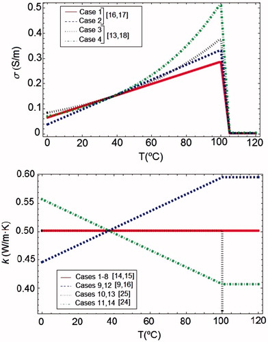
The most commonly used mathematical function for σ in RFA models is a piecewise function which uses different mathematical expressions according to the temperature range. First, at temperatures below 100 °C, σ increases. However, there are discrepancies about the rate of this increase, from +1.5%/°C [15] to +2%/°C [8], and about the increase type, linear [16,17] or exponential [13,18].

At temperatures above 100 °C vaporisation occurs and desiccation implies a rapid drop of σ. There are also discrepancies about the rate of this drop: Byeongman and Aksan [13] considered that σ decreases by approximately two orders of magnitude between 105 °C and 110 °C, Haemmerich et al. [14] assumed a rapid drop by a factor of 10,000 between 100 °C and 102 °C, and Pätz et al. [19] considered a discontinuous drop to a value close to zero. Here we have studied the effect of the following variations of σ with temperature (see Table I):

1. For temperatures below 100 °C, two increase rates: 1.5 and 2%/°C, and two increase types: linear and exponential.

2. For temperatures above 100 °C, two drop rates: two and four orders of magnitude between 100 °C and 105 °C.

These combinations of σ allowed up to eight cases in which k was assumed to be constant (see set 1 in Table I). In Figure 1 we represented the different functions used for σ in the case of a drop rate of two orders.

Figure 1. Representation of the functions used for modelling the thermal dependence of σ and k. In the case of σ was showed only a two order drop for T > 105 °C. Legends specify some references in which these kinds of functions of σ and k are used.

Temperature dependence of thermal conductivity (k)

Most RFA theoretical models have used a constant value for k [14,15,17,20–22], probably due to the fact that changes in k with temperature are not so marked as in σ [10,23]. Models considering k temperature dependence used a piecewise continuous function. The great discrepancies between these functions are found for temperatures up to 100 °C [24]. The most commonly used approximation considered a linear increase of k [9,16], but a decreasing function for k, which depends on the fraction of water vaporised has also been proposed [24]. Above 100 °C, k has been assumed to be constant [13]. A few studies modelled the temperature dependence of k with a non-continuous piecewise function which considered two different values for k before and after water vaporisation temperature [25].

We have considered the following variations of k with temperature (see Table I).

1. A constant value (see set 1 in Table I).

2. A linear increase rate of 1.5%/°C for temperatures below 100 °C, and a constant value for temperatures above 100 °C [13].

3. A different value before (0.502 W/m °C) and after (0.092 W/m °C) water vaporisation [25], i.e. a different value for each phase, liquid and gas.

4. A linear drop rate of −1.5%/°C for temperatures below 100 °C, and a constant value for temperatures above 100 °C [24].

In Figure 1 we represented the different functions used to model the thermal dependence of k.

Description of the model of RF hepatic ablation

To compare the effect of the different combinations of the mathematical functions presented in the previous section, we considered a theoretical RF hepatic ablation model which consisted of a fragment of hepatic tissue and an internally cooled electrode. Figure 2 shows the geometry and dimensions of the theoretical model. The problem presented axial symmetry and hence a two-dimensional analysis was conducted. The model included three different materials: plastic partially covering the electrode, a metallic electrode and a fragment of hepatic tissue. The dispersive electrode was modelled as an electrical condition on boundaries at a distance from the active electrode. The model was based on a coupled thermo-electric problem which was solved numerically using COMSOL Multiphysics software (COMSOL, Burlington MA, USA). The bioheat equation [26] was used as the governing equation of the thermal problem. The enthalpy method [13,25] was considered to modify the bioheat equation and hence to incorporate the phase change [22,27] as follows: where ρ is tissue density, h enthalpy, T temperature, t time, k thermal conductivity, q heat source produced by RF power, and Q_p heat loss from blood perfusion. For biological tissues, enthalpy is related to tissue temperature by the following expression [25,28]: where ρ_i and c_i are tissue density and specific heat of tissue in liquid phase (i = l, i.e. tissue at temperatures below 100 °C) and the post-phase-change tissue (i = g, i.e. tissue at temperatures above 100 °C), h_fg is the product of water latent heat of vaporisation and water density at 100 °C and C is tissue water content inside the liver (68%) [19]. The notation h(99) and h(100) refers to enthalpy at 99 and 100 °C, respectively. The characteristics of materials used in the model are shown in Table II [12,19,29,30].

Figure 2. Geometry of the two-dimensional theoretical model (out of scale and dimensions in mm) and electrode detail. The domain is divided into three zones: plastic portion of the electrode, metallic electrode and hepatic tissue.

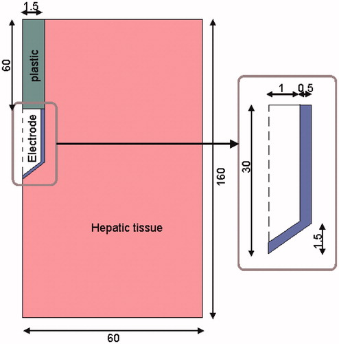
Table II. Characteristics of the materials used in the theoretical model [12,19,29,30].

Tissue/material	σ (S/m)	k (W/m K)	ρ(kg/m^3)	c (J/kg K)
Electrode	7.4 × 10^6	15	8 × 10^3	480
Plastic	10^−5	0.026	70	1045
Liver	0.132^a	0.502^b	1080^c	3455^c
			370^d	2156^d

σ, electric conductivity; k, thermal conductivity; ρ, density; c, specific heat.

^aAssessed at 17 °C. This allows initial impedance (≈100 Ω) to match the experimental mean value obtained from [30].

^bAssessed at 37 °C [12].

^cTissue in liquid phase.

^dTissue in gas phase.

Firstly, we conducted a set of simulations including cases 1 to 8 (see Table I) in order to assess the effect of σ. From the results of this first set we selected the two most different cases of impedance evolution, i.e. those with the earliest and latest roll-offs, roll-off being the time at which tissue impedance is 30 Ω higher than the initial. We then set the mathematical function used for σ in these extreme cases (1 and 4, see results) and conducted a second set of simulations varying k by means of different temperature-dependent functions (cases 9 to14).

The heat source from RF power q (Joule losses) was given by q = σ|E|², where E is an electric field which was obtained from the electrical problem. The Laplace equation ▿²V = 0 was the governing equation for the electric problem, V being the voltage. The electric field was calculated by means of E = −▿V. We used a quasi-static approach, i.e. tissues were considered as purely resistive due to the value of the frequencies used in RF (≈500 kHz) and for the geometric area of interest (electrical power is deposited in a very small zone close to the electrode) [31]. The blood perfusion term Q_p was obtained from: where ρ_b is density of blood (1000 kg/m³) [14], c_b specific heat of blood (4180 J/Kg K) [8], T_b blood temperature (37 °C), ω_b blood perfusion coefficient (6.4 × 10⁻³s⁻¹) [32] and β is a coefficient which took the values of 0 and 1, depending on the value of the local thermal damage Ω: β = 0 for Ω ≥ 1, and β = 1 for Ω < 1. The parameter Ω was assessed by the Arrhenius damage model [32], which associates temperature with exposure time using a first-order kinetics relationship: where R is the universal gas constant, A is a frequency factor and ΔE is the activation energy for the irreversible damage reaction. The parameters A and ΔE for liver were A = 8 × 10³⁹s⁻¹ and ΔE = 2.577 × 10⁵J/mol [33]. We employed the thermal damage contour D63 to compute the lesion dimension contour, which corresponds to Ω = 1 (63% probability of cell death) [21].

Thermal boundary conditions were null thermal flux in the transversal direction to the symmetry axis and constant temperature of 37 °C in the dispersive electrode. Initial temperature of the tissue was considered to be 37 °C. The cooling effect produced by the liquid circulating inside the electrode was modelled using a thermal convection coefficient h with a value of 3366 W/K m² and a coolant temperature of 10 °C following the Newton’s law of cooling. The value of h was calculated by considering a length of 30 mm and a flow rate of 45 mL/min through an area of 1.57 × 10⁻⁶ m², which is equivalent to half of the cross-section of the inner diameter of the electrode (see Figure 2).

Electrical boundary conditions were zero current density in the transverse direction to the symmetry axis and inside the electrode and zero voltage in the dispersive electrode. The modelled pulsed RF protocol consisted of the application of 80 V up to roll-off time. Impedance evolution up to roll-off was used to compare the different mathematical functions, since this time is closely related to the time when dehydrated tissue reaches the middle zone of the electrode [30], i.e. when the area close to the electrode reaches a temperature around 100 °C. Once roll-off occurs, power is switched off for 15 s and then a new 80 V pulse is again applied until the next roll-off. This procedure, common in clinical practice, is repeated for a period of 6–12 min. The simulations lasted for up to 6 min and the protocol was implemented by means of a connection between COMSOL and MATLAB (MathWorks, Natick, MA).

The model mesh was heterogeneous, with a finer mesh size at the electrode–tissue interface, where the highest electrical and thermal gradients were expected. All the mesh elements used were triangular, and areas ratios varied between 2.5e-7 and 2.85e-5 m². The size of the finer mesh was estimated by a convergence test. We used the value of the maximum temperature (T_max) reached in the liver at the first roll-off time as a control parameter in these analyses. When there was a difference of less than 0.5% in T_max between simulations we considered the former mesh size as appropriate. The final total number of elements and degrees of freedom were 4991 and 30 330, respectively. Analogously, we used a similar convergence test to estimate the optimal time-step. In the case of the time-step we used an adaptive scheme since we let the time-stepping method choose time steps freely.

All computer simulations were performed with a Dell T7500 workstation with Six Core, 2.66 GHz Xeon processors and 48 GB RAM running on a Windows 7 Professional 64 bit operating system.

Results

The first roll-off time and the follow-ups to 12 min were registered for each case. In all cases we observed that after the first roll-off the subsequent roll-offs occurred at intervals of 25.7 ± 2.1 s. Figure 3 shows impedance evolution up to the first roll-off in some cases with σ modelled in different ways. Figure 3A shows the cases in which the increase of σ with temperature up to 100 °C was modelled for two increase rates (1.5 and 2%/°C) and types (linear and exponential). In all these cases we considered a two-order drop when T > 100 °C (see Table I). In general, the first roll-off occurred earlier in cases with exponential (3 and 4) than linear increase (1 and 2), with a difference of 4.8%. Moreover, roll-off occurred earlier when the increase rate was 2%/°C (cases 2 and 4) compared to 1.5%/°C (cases 1 and 3), with a difference of 7%. Consequently, the extreme cases were 1 (latest first roll-off) and 4 (earliest first roll-off) with time differences of 11.5% in achieving first roll-off. Figure 3B shows the impedance evolution for these extreme cases and the same cases with a four-order drop in T > 100 °C in σ (cases 5 and 8, respectively). Here, the differences were almost negligible (<1.5%).

Figure 3. (A) Impedance evolution to the first roll-off in cases 1 to 4. (B) Impedance evolution to the first roll-off in cases 1, 4, 5 and 8. The only characteristic which varies in both figures is σ, in accordance with Table I.

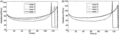
Figure 3 also shows that impedance evolution can be divided into three zones: 1) initial drop; 2) plateau; and 3) sudden increase up to roll-off. Figure 3A shows that in cases with linear increase (cases 1 and 2) the drop and increase slopes of the impedance plot were smaller than with exponential increase (cases 3 and 4). Moreover, for the same type of increase, the drop and increase slopes of the impedance plot were smaller when the increase rate was 1.5%/°C compared to 2%/°C. In contrast, Figure 3B shows that there are no differences in impedance evolution between a two-order or four-order drop in σ.

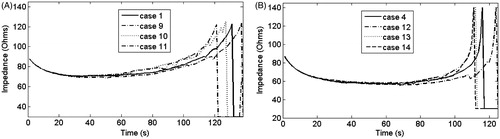
In the second set of simulations we considered the extreme cases from the first set (cases with the earliest and latest roll-offs, 1 and 4) and then varied k according to cases 9 to 14, (see Table I). Figure 4 shows the impedance evolution up to first roll-off in these cases. Figure 4A shows the impedance evolution in cases 1, 9, 10 and 11, i.e. with an extreme case of σ and different combination of k. Figure 4B shows the impedance evolution of cases 4, 12, 13 and 14, which correspond with the complementary extreme case of σ and the same combinations of k. In both figures it can be seen that in comparison with the cases in which k was constant (1 and 4), the first roll-off was achieved later in cases in which k increases with respect to the initial value (9 and 12), and earlier in cases in which k decreases linearly with respect to the initial value (11 and 14), with differences of ≈5%. These last differences increased by 1–2% when there was a sudden drop in k (10 and 13), i.e. a different value of k before and after 100 °C. Moreover, in all cases the drop and increase slopes of the impedance plot were similar, and changes in impedance evolution were only observed during the time in which impedance started to increase.

Figure 4. (A) Impedance evolution in cases 1, 9, 10 and 11. (B) Impedance evolution in cases 4, 12, 13 and 14. A different mathematical function for k was used in each case, in accordance with Table I.

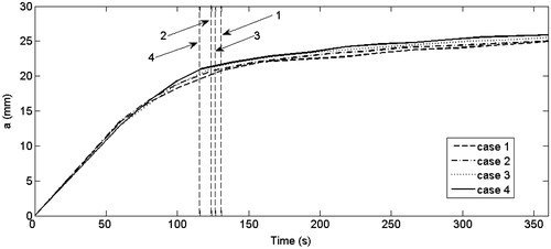
Finally, in order to assess the impact of the method of modelling the temperature dependence of σ and k on lesion dimensions, the evolution of the lesion short diameter (transverse diameter) for cases 1 to 4 was plotted for a period of 6 min (see Figure 5). In Figure 5 the dashed vertical lines indicate the time at which the first roll-off occurred in each case. The maximum difference was 6% between cases 1 and 4 at ≈220 s. This difference was only 3.5% at 6 min. The same comparison was made for cases 5 to 8, 9 to 11 and 12 to 14 (not shown) and differences in the lesion short diameter were always smaller. We also observed that a longer time for the first roll-off was not related to a greater lesion diameter (Figure 5). Indeed, when the first roll-off occurred, the lesion diameter was similar in all cases and its value was ≈75% of the lesion diameter at the end of ablation. Figure 5 also shows that the growth rate of the lesion decreased linearly with time.

Figure 5. Evolution of the lesion short diameter (a) throughout 360 s for cases 1 to 4 (see Table I for details). Dashed lines represent the time in which the first roll-off was achieved in each case.

The computational time required to obtain the solutions was almost the same in all the cases considered. Cases 1–8 were similar from a computational point of view, since a piecewise temperature-dependent function was used for σ and a constant value for k. We noticed that the computational time was around 5% longer in cases 9–14, in which a piecewise temperature-dependent function was used for k.

Discussion

In this study the different approaches employed by other authors to theoretically model the temperature dependence of σ and k during RFA were reviewed and compared, including those involving the electrical and thermal performance of tissue around 100 °C. The impedance evolution up to first roll-off was used to compare the different approaches, since impedance increases abruptly and the subsequent roll-off occurs when the electrode is completely surrounded by dehydrated tissue (≈100 °C) [30]. The evolution of the short diameter of the thermal lesion for up to 6 min was also used as a comparison.

We consider that the findings of this study can be explained by the thermo-electrical performance of the tissue around the electrode. Impedance evolution up to the first roll-off is divided into three zones (intervals) which are related to the temperature evolution of tissue surrounding the electrode (Figure 6). To understand the behaviour of impedance in each zone it is important to be aware that 1) impedance and σ are somewhat inversely related, and 2) the value of σ is a characteristic of every point in the tissue, while impedance is the result of a spatial integral which takes into account the value of σ at all points in the tissue. Thus σ increases at points located at the edges of the electrode (distal and proximal) in the early stages of RFA, due to the rapid rise in temperature in this zone, after which impedance gradually decreases (zone 1). As the temperature of the tissue around the electrode increases, there is a balance between points with temperatures at and above 100 °C. In the former, σ drops abruptly and in the latter σ is increasing. This situation causes an impedance plateau (zone 2). Finally, when the tissue around the electrode middle zone rises to a temperature over 100 °C, i.e. when the electrode is completely surrounded by dehydrated tissue, impedance increases abruptly and roll-off occurs (zone 3) [30]. According to this behaviour, it seems obvious that when σ grows slowest (i.e. linear type increase and 1.5%/°C rate) the changes in impedance are more gradual, the drop and increase slopes of impedance evolution are smaller and roll-off occurs later.

Figure 6. Two-dimensional tissue temperature distribution during RFA and impedance evolution. The impedance progress can be divided into three intervals: 1) initial impedance drop; 2) impedance plateau; and 3) abrupt increase of impedance. These zones are related to the physical conditions of the tissue during the RFA process [30].

On the other hand, as k measures the tissue’s ability to conduct heat, then when the value of k is lower, around 100 °C, (i.e. a sudden drop in k when T > 100 °C and when k decreases linearly up to 100 °C), the tissue is maintained at high temperatures for a longer time, so that there is a larger amount of tissue in which σ drops at the same time, consequently roll-off occurs earlier. This also agrees with the results obtained by Tungjitkusolmun et al. [8] in the computer modelling of RF cardiac ablation, in which they found that a drop in k implied that the maximal temperature of 100 °C was reached earlier. A rise in k likewise involved a drop in the maximum temperature reached at the end of a preset time [34].

When we studied the evolution of the short diameter of the thermal lesion we found that a large part of the lesion volume is formed at the first roll-off time (Figure 5) and thus used this time to compare cases. We also observed that longer first roll-off times were not necessarily related to bigger lesions. It can therefore be said that the different mathematical functions used to model σ and k give different first roll-off times (differences up to 11.5%) but not final lesion size after 6 min ablation (differences of 3.5% in short diameter). Also, the differences in lesion evolution are only noticeable from the first until approximately the third roll-off, after which they become negligible. This undoubtedly has clinical implications, since the computer results suggest that the lesion is almost complete after three roll-off episodes and experiences little change from this point on.

One of the limitations of this study is that we focused on piecewise mathematical functions as they are the most commonly used. However, it must be said that other kinds of mathematical functions can be used to model these characteristics in RFA. Pearce et al. [27] considered water as the most thermodynamically active tissue constituent and both their formulation and the functions used to model σ and k take into account the tissue water content. As regards σ, some studies have considered a temperature dependence based on a polynomial relation derived from NaCl solutions [21,35]. Ji and Brace [36] recently have suggested that variations in liver electrical conductivity at temperatures near 100 °C are best modelled using a sigmoid function for microwave thermal ablation. Watanabe et al. [37] studied and modelled k temperature dependence using three different piecewise functions to those used in our study.

Our study did not include any case in which σ was constant with temperature, since it had previously been demonstrated that this dependence has to be included in the models to achieve realistic results [38]. Likewise, we always considered the latent heat associated with the liquid–gas phase change when tissue reached 100 °C (in particular the enthalpy method [25]). Excluding this heat from the governing equation would considerably reduce the time to first roll-off. Neither of these approaches (using for σ a constant value with temperature and excluding latent heat) was considered, as they do not accurately reflect what really happens.

Our aim was not to choose the most suitable function to represent the temperature dependence of σ and k, which would need additional experimental studies outside the scope of this work. Although it has been demonstrated that both characteristics depend on temperature, no studies have been carried out on the type of function that best represents this dependence. In all the cases considered, a similar trend was observed in the σ growth up to 100 °C, a sudden drop between 100–105 °C, after which it remains constant at a very low value. However, there is somewhat more uncertainty in the case of k. Although we have found some studies (e.g. [37]) on the temperature dependence of k, a deeper study of this issue is required. A good result in this area would provide the necessary information for the accurate modelling of σ and k. The current lack of this information means that it necessary to assess the impact of the common mathematical functions used to model the temperature dependence of σ and k in RFA. Temperature profiles obtained in the simulations are relevant and typically found in a RFA regime, which validates our results in other RF problems (see for example [21] and [35]).

Conclusions

Although our main objective was to review and assess the impact of the mathematical functions most commonly used to model the temperature dependence of σ and k in RFA, our findings in the case of RFA modelling allow us to suggest the following:

1. The temperature dependence of σ below 100 °C can be modelled equally well either by using a linear or exponential increase or an increase rate of between +1.5%/°C and +2%/°C.

2. Once temperature reaches 100 °C, the change in σ caused by dehydration can be modelled equally well by using an abrupt drop of either two or four orders of magnitude between 100 °C and 105 °C.

3. The temperature dependence of k can be ignored, and hence a constant value can be used, since the different approaches proposed in previous modelling studies provide similar results.

4. The COMSOL computing time was similar in all cases.

In the context of this study, the term ‘equally’ means that the computed lesion short diameter after 6 min ablation differs by less than 3.5%. These conclusions could be useful for groups conducting research on RFA modelling using software with limited options on the temperature dependence of σ and k.

Declaration of interest

This work received financial support from the Spanish Plan Nacional de I + D + I del Ministerio de Ciencia e Innovación, grant no. TEC2011-27133-C02-01, and from the PAID-06-11 UPV, grant ref. 1988. The authors alone are responsible for the content and writing of the paper.

References

- Benoist S, Nordlinger B. Radiofrequency ablation in liver tumors. Ann Oncol 2004;15:313–17
- McAchran SE, Lesani OA, Resnick MI. Radiofrequency ablation of renal tumors: Past, present and future. Urology 2005;66:15–22
- Di Staso M, Zugaro L, Gravina GL, Bonfili P, Marampon F, Di Nicola L, et al. A feasibility study of percutaneous radiofrequency ablation followed by radiotherapy in the management of painful osteolytic bone metastases. Eur Radiol 2011;21:2004–10
- Sharma R, Wagner JL, Hwang RF. Ablative therapies of the breast. Surg Oncol Clin N Am 2011;20:317–39
- Savoie PH, Lopez L, Simonin O, Loubat M, Bladou F, Serment G, et al. Two-years follow-up of radiofrequency thermotherapy for urination disorders due to benign prostatic hyperplasia [in French]. Prog Urol 2009;19:501–6
- Akeboshi M, Yamakado K, Nakatsuka A, Hataji O, Taguchi O, Takao M, et al. Percutaneous radiofrequency ablation of lung neoplasms: Initial therapeutic response. J Vasc Interv Radiol 2004;15:463–70
- Berjano EJ. Theoretical modeling of epicardial radiofrequency ablation: State-of-the-art and challenges for the future. Biomed Eng Online 2006;5:24
- Tungjitkusolmun S, Woo EJ, Cao H, Tsai JZ, Vorperian VR, Webster JG. Thermal-electrical finite element modeling for radio frequency cardiac ablation: Effects of changes in myocardial properties. Med Biol Eng Comput 2000;38:562–8
- Shahidi AV, Savard P. A finite element model for radiofrequency ablation of the myocardium. IEEE Trans Biomed Eng 1994;41:963–8
- Solazzo SA, Liu Z, Lobo SM, Ahmed M, Hines-Peralta AU, Lenkinski RE, et al. Radiofrequency ablation: importance of background tissue electrical conductivity – An agar phantom and computer modeling study. Radiology 2005;236:495–502
- Gabriel C, Gabriel S, Corthout E. The dielectric properties of biological tissues: I. Literarure survey. Phys Med Biol 1996;41:2231–49
- Duck F. Physical properties of tissue – A comprehensive reference book. New York: Academic Press; 1990
- Byeongman J, Aksan A. Prediction of the extent of thermal damage in the cornea during conductive thermokeratoplasty. J Therm Biol 2010;35:167–74
- Haemmerich D, Chachati L, Wright AS, Mahvi DM, Lee FT, Webster JG. Hepatic radiofrequency ablation with internally cooled probes: Effect of coolant temperature on lesion size. IEEE Trans Biomed Eng 2003;50:493–9
- Jarrard J, Wizeman B, Brown RH, Mitzner W. A theoretical model of the applications of RF energy to the airway wall and its experimental validation. Biomed Eng Online 2010;9:81
- Dodde RE, Miller SF, Geiger JD, Shih AJ. Thermal-electric finite element analysis and experimental validation of bipolar electrosurgical cautery. J Manuf Sci Eng 2008;130:021015-1–8
- Lau M, Hu B, Werneth R. A theoretical and experimental analysis of radiofrequency ablation with a multielectrode, phased, duty-cycled system. Pacing Clin Electrophysiol 2010;33:1089–100
- Berjano EJ, Alió JL, Saiz J. Modeling for radio-frequency conductive keratoplasty: Implications for the maximum temperature reached in the cornea. Physiol Meas 2005;26:157–72
- Pätz T, Kröger T, Preusser T. Simulation of radiofrequency ablation including water evaporation. IFMBE Proceedings 2009;25/IV:1287–90
- Jain MK, Wolf PD. A three-dimensional finite element model of radiofrequency ablation with blood flow and its experimental validation. Ann Biomed Eng 2000;28:1075–84
- Chang IA, Nguyen UD. Thermal modeling of lesion growth with radiofrequency ablation devices. Biomed Eng Online 2004;3:27
- Yang D, Converse MC, Mahvi DM, Webster JG. Expanding the bioheat equation to include tissue internal water evaporation during heating. IEEE Trans Biomed Eng 2007;54:1382–8
- Bhavaraju NC, Valvano JW. Thermophysical properties of swine myocardium. Int J Thermophys 1999;20:665–76
- Baldwin SA, Pelman A, Bert JL. A heat transfer model of thermal balloon endometrial ablation. Ann Biomed Eng 2001;29:1009–18
- Abraham JP, Sparrow EM. A thermal-ablation bioheat model including liquid-to-vapor phase change, pressure- and necrosis-dependent perfusion, and moisture-dependent properties. Int J Heat Mass Transfer 2007;50:2537–44
- Pennes H. Analysis of tissue and arterial blood temperatures in the resting human forearm. J Appl Physiol 1948;85:5–34
- Pearce J, Panescu D, Thomsen S. Simulation of diopter changes in radio frequency conductive keratoplasy in the cornea. WIT Trans Biomed Health 2005;8:469–77
- Zhao G, Zhang HF, Guo XJ, Luo DW, Gao DY. Effect of blood flow and metabolism on multidimensional heat transfer during cryosurgery. Med Eng Phys 2007;29:205–15
- Berjano EJ, Burdío F, Navarro AC, Burdío JM, Güemes A, Aldana O, et al. Improved perfusion system for bipolar radiofrequency ablation of liver: Preliminary findings from a computer modeling study. Physiol Meas 2006;27:N55–66
- Trujillo M, Alba J, Berjano E. Relation between roll-off occurrence and spatial distribution of dehydrated tissue during RF ablation with cooled electrodes. Int J Hyperthermia 2012;28:62–8
- Doss JD. Calculation of electric fields in conductive media. Med Phys 1982;9:566–73
- Chang IA. Considerations for thermal injury analysis for RF ablation devices. Biomed Eng Online 2010;4:3-12
- Jacques S, Rastegar S, Thomsen S, Motamedi M. The role of dynamic changes in blood perfusion and optical properties in laser coagulation of tissue. IEEE J Sel Top Quantum Electron 1996;2:922–33
- Berjano EJ, Saiz J, Ferrero JM. Radio-frequency heating of the cornea: Theoretical model and in vitro experiments. IEEE Trans Biomed Eng 2002;49:196–205
- Barauskas R, Gulbinas A, Barauskas G. Investigation of radiofrequency ablation process in liver tissue by finite element modeling and experiment. Medicina (Kaunas) 2007;43:310–25
- Ji Z, Brace CL. Expanded modeling of temperature-dependent dielectric properties for microwave thermal ablation. Phys Med Biol 2011;56:5249–64
- Watanabe H, Yamazaki N, Kobayashi Y, Miyashita T, Fujie MG. Temperature dependence of thermal conductivity of liver based on various experiments and a numerical simulation for RF ablation. Conf Proc IEEE Eng Med Biol Soc 2010;2010:3222–8
- Labonté S. Numerical model for radio-frequency ablation of the endocardium and its experimental validation. IEEE Trans Biomed Eng 1994;41:108–15