Validation of MR thermometry: Method for temperature probe sensor registration accuracy in head and neck phantoms

Abstract

Purpose: Magnetic resonance thermometry (MRT) is an attractive means to non-invasively monitor in vivo temperature during head and neck hyperthermia treatments because it can provide multi-dimensional temperature information with high spatial resolution over large regions of interest. However, validation of MRT measurements in a head and neck clinical set-up is crucial to ensure the temperature maps are accurate. Here we demonstrate a unique approach for temperature probe sensor localisation in head and neck hyperthermia test phantoms. Methods: We characterise the proton resonance frequency shift temperature coefficient and validate MRT measurements in an oil–gel phantom by applying a combination of MR imaging and 3D spline fitting for accurate probe localisation. We also investigate how uncertainties in both the probe localisation and the proton resonance frequency shift (PRFS) thermal coefficient affect the registration of fibre-optic reference temperature probe and MRT readings. Results: The method provides a two-fold advantage of sensor localisation and PRFS thermal coefficient calibration. We provide experimental data for two distinct head and neck phantoms showing the significance of this method as it mitigates temperature probe localisation errors and thereby increases accuracy of MRT validation results. Conclusions: The techniques presented here may be used to simplify calibration experiments that use an interstitial heating device, or any heating method that provides rapid and spatially localised heat distributions. Overall, the experimental verification of the data registration and PRFS thermal coefficient calibration technique provides a useful benchmarking method to maximise MRT accuracy in any similar context.

• Control systems engineering/treatment optimisation
• imaging (i.e. PET, CT, MRI)
• non-invasive thermometry
• invasive thermometry
• quality assurance

Introduction

Thermotherapy procedures involve increasing or decreasing the temperature of in vivo tissue to prompt a biological response (e.g. increased vascularisation, cell necrosis) when sufficient thermal dose has been delivered. Thermal coagulation can be achieved by raising the tissue temperature by 13–40 °C for short durations (<1 min). Raising cells to this temperature kills them through protein denaturation. Examples of procedures in this category include focused ultrasound (FUS) ablation, laser ablation, and radiofrequency (RF) ablation [1]. An example of a more moderate heating procedure is adjuvant RF hyperthermia (RF-HT) [2]. Here, the temperature rise is between 3–6 °C but held for a longer (>30 min) duration. Hyperthermia induces a number of mechanisms that have additive and supra-additive effects on radiotherapy and chemotherapy [3].

Phase III studies [4–6], including many head and neck specific [7–9], have shown that RF-HT used in conjunction with other therapy modalities such as radio- or chemotherapy significantly increases the efficacy of cancer treatment. RF-HT typically involves invasive placement of temperature probes in catheters for thermometry. In the head and neck region (i.e. oral cavity, nasal cavity, pharynx and larynx), complex anatomy requires non-linear catheter trajectories to safely reach tumours [10]. The prevalence of thermo-sensitive tissue in this area requires that there is no stray heating outside targeted areas. This becomes challenging when the spatial resolution of temperature measurements is limited by the small number of catheters (∼4) that can be safely inserted. Magnetic resonance thermometry (MRT) was demonstrated to be feasible during RF-HT [11] and has proven to be an effective and non-invasive method to monitor temperature changes in vivo [12–16]. In thermotherapy procedures, MRT provides fast and accurate measurements of 3D temperature and thermal dose over a large region of interest with high spatial resolution.

Temperature measurement through MR can be done many ways. Longitudinal relaxation time (T₁) [17,18], the diffusion constant of water [19,20], and the proton resonance frequency shift (PRFS) [13,21,22] of water-based tissues have been shown to exhibit measurable temperature dependence. Of these, the latter is most commonly used for its ease of measurement and linear temperature dependence. In the PRFS method, the temperature change (ΔT) is calculated based on the relation shown in Equation 1: where is the difference between phase images (acquired before and after temperature change), γ is the gyromagnetic ratio, B₀ is the static magnetic field strength, TE is the echo time of the phase images, and α is the PRFS thermal coefficient (the PRF change per degree Celsius) reported in units of ppm/°C. The accuracy of calculating a temperature change using the PRFS method is greatly dependent on the PRFS thermal coefficient (α -parameter). An incorrect α value will lead to an error in the estimation of an accurate temperature distribution. This may have serious consequences as the temperature in healthy thermo-sensitive tissue may be underestimated, or the thermal dose in the target region overestimated, potentially leading to toxicity or reduced therapeutic effect.

Although work done by Peters et al. [23] shows some degree of tissue-type independence for the α value in ex vivo water-based animal tissues, many discrepancies remain in current literature for this parameter. For example, recent work by Shrivastava et al. [24] is based on an α value of ∼0.015 ppm/°C, while in other works, values of ∼0.01 ppm/°C [12,25,26] are assumed. In general, most groups assume α values in the range of 0.0096–0.015 ppm/°C. For a given phase difference, this range of α may yield a 56% spread of values for the computed temperature rise, e.g. ΔT = 6 °C to 9.36 °C calculated from Equation 1. Since the success of thermal therapies depends on accurate temperature maps, accurate characterisation of the α-parameter is crucial. Such characterisation may be challenging when it is difficult to accurately determine probe locations in the MR image coordinate space. These misalignments degrade MRT validation and the α characterisation, especially for procedures with spatially localised heat distributions where a small spatial shift in a probe’s location may yield a significantly different temperature reading due to the strong thermal gradients.

In any clinical thermotherapy method, absolute temperature accuracy relies on the use of invasive temperature probes for measuring local temperature during a heating experiment. In order to validate MRT as a non-invasive replacement for invasive probes, one must first show exact registration between the two data types. This involves both precise temperature sensor localisation in the MRI coordinate space, and accurate calibration of the material-specific α-parameter for the reasons mentioned above.

In this study we present an experimental method that can be used for temperature sensor localisation, and calibration of the α-parameter, thereby mitigating these variables’ impact on registration errors between temperature probe and MRT data. The method itself is straightforward, but subtleties must be properly considered for precise measurement. The results establish a benchmarking tool for MRT validation experiments.

Materials and methods

Phantoms

Two separate phantoms were used in this study, each with the general structure shown in Figure 1. Both phantoms had an inner cylinder (diameter = 100 mm) that held a human muscle-mimicking material composed of either a gadolinium-doped polysaccharide (TX-151 or ‘superstuff’) made with 86.51% deionised water, 2.72% agar, 6.74% polyethylene powder, 2.47% TX-151, 1.14% formaldehyde, 0.41% sodium chloride, 0.08 mL/kg 1 mM Gd-DO3A-butrol (Gadovist, Bayer, Germany), or a ‘gelatin’ made with 73.5% deionised water, 13.72% gelatin (Bloom 22, Sigma-Aldrich, St Louis, MO), 8.52% sunflower oil, 0.46% surfactant (Triton, Sigma-Aldrich), 0.6% sodium chloride, 3.19% formaldehyde [27]. The outer layer (total diameter 135 mm) contained pure sunflower oil for both phantoms. Overall, the inner region material properties were designed to simulate in vivo tissues. Measured specific heat capacity, density, and relative dielectric permittivity closely match reported values of in vivo tissues. Specific heat capacity and density respective values were of 3387 J/kg °C, 1045 kg/m³ for gelatin, and 3709 J/kg °C, 1007 kg/m³ for superstuff. The specific heat of each phantom material was measured using a differential scanning calorimeter (DSC) over the temperature range from 10–50 °C, and the thermal conductivity of each phantom material was obtained from transient temperature measurements fitted to a one-dimensional heat transfer equation as in Yuan et al. [28]. The thermal conductivities of both interior phantom recipes were measured to be ∼40% higher than expected, giving values of 0.515 W/m °C for gelatin, and 0.565 W/m °C for superstuff. Dielectric properties were measured by a vector network analyser with a dielectric assessment probe over a frequency range from 64 MHz (proton resonance frequency at 1.5T) to 434 MHz (HT applicator working frequency). Resulting relative dielectric permittivity and dielectric conductivity values at 434 MHz were 57.4, 1.07 S/m for gelatin phantom and 60.6, 0.85 S/m for superstuff. Dielectric conductivity at 64 MHz was 0.93 S/m and 0.79 S/m for gelatin and superstuff respectively. T₁, and were measured at 1.5 T for the phantom interiors. T₁ images were acquired using a 2D axial inversion recovery (IR) sequence at the following TI values: 3000, 2600, 2200, 1800, 1400, 1000, 700, 400, 200, 50 with all times in ms. Other parameters included flip angle (θ) 90°, TE 4 ms, TR 5000 ms, FoV 40 × 40 cm², matrix size 128 × 128, slice thickness 10 mm, and 1 signal average (NEX). The T₁ values of 736 and 806 ms were used to set the Ernst angle in all gradient-spoiled imaging sequences used for the gelatin and superstuff phantoms respectively. values for both phantoms were ∼30 ms. images were acquired using a 2D axial spoiled-gradient echo (SPGR) sequence at the following TE values: 210, 200, 180, 140, 100, 60, 40, 20, 10 with all times in ms. Other parameters included θ 29°, TR 220 ms, FoV 40 × 40 cm², matrix size 128 × 128, slice thickness 10 mm, NEX 1. All MR images were acquired on a 1.5 T GE MR450w scanner (GE Healthcare, Waukesha, WI).

Figure 1. Head and neck hyperthermia phantom set-up. (a) Top view of phantom. (b) Side view of phantom showing catheter path. (c) Fibre-optic temperature probe strand containing four equi-spaced temperature sensors distributed along its length. (d) Illustration of phantom set-up: the temperature probe strand from (c) is inserted into the catheter track which has a non-linear trajectory through the oil and phantom interior. Right magnification box: due to the bending catheter trajectory it is common for the temperature probe tip to become stuck before reaching the actual catheter tip. This will lead to temperature probe/MRT data misregistration (see text for further discussion).

Catheter mapping

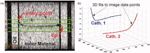
Brachytherapy delivery catheters (William Cook, model P4.1-CE-50-SFT-NS-0, internal diameter 0.89 ± 0.03 mm, outer diameter 1.32 ± 0.03 mm) were inserted through the gelatin and superstuff phantoms (Figure 1a, b, and d) and imaged with a 3D fast-SPGR sequence (TE 3.3 ms, TR 6.9 ms, θ 8°, FoV 33 × 33 cm², matrix size 512 × 512, NEX 2, slice thickness 2 mm). The contrast between the proton-rich inner material and the signal-void region of the hollow catheter tube (Figure 2a) was used to manually extract points that trace the path of the catheter. Spatial coordinates referenced according to anterior–posterior (A/P or ±y), superior–inferior (S/I or ±z), and right–left (R/L or ±x) locations were exported to Matlab (Mathworks, Natick, MA). Three-dimensional cubic spline curve fitting was performed on these points to generate the 3D trajectory of the catheter/temperature probe path. Each fitted curve was parameterised by the length from the tip of the catheter, which facilitated identification of the locations of four temperature sensors distributed equally along each fibre-optic probe strand (Figure 1d).

Figure 2. 3D spline catheter mapping. (a) Coronal fast-SPGR image showing the catheter in the phantom. For images such as this, the tip localisation was within <1 mm accuracy (in-plane uncertainty in the catheter tip was within 1 pixel on a 512×512 matrix with 33 cm FoV). Also shown here are the approximate axial slice locations for the SPGR images used in the MRT calculations. Axial slices are labelled 1–4. (b) Spline fits for catheter/temperature probe localisation. Data points are extracted from images such as (a) to reconstruct the catheters in MR image coordinate space.

Heating experiments and thermometry

The phantom was heated with phase-coherent RF radiation at 434 MHz using an MR-compatible laboratory prototype of the HYPERcollar RF hyperthermia applicator [29]. The heat applicator consists of two rings of six patch antennas optimised to give a minimum antenna reflection coefficient (S₁₁) at 434 MHz. The S₁₁ was always measured lower than −10 dB for any antenna. Each ring of antennas was driven with 25 W applied power by an individual RF power amplifier (RFPA). The applied power is referring to the RFPA output power after consideration of hardware losses (e.g. cables, connectors). Each channel of six antennas received 25 W input power for approximately 6 min. All antennas are driven with identical RF signal phase shifts, i.e. inter-antenna relative phase shift of 0°. Experiments were performed such that heating and scanning never occurred simultaneously, i.e. RF power to the HYPERcollar was turned off when MRT data was acquired. RF power to HYPERcollar applicator was turned on to resume heating after each MRT scan (∼12 s per scan) was completed. Fibre-optic temperature probe sensors (FISO, Quebec, Canada, model FOT-NS-577C, serial numbers: THC0023E, THC0022B, THC0022A, THC0022C, OD = 0.8 ± 0.05 mm, ± 0.1 °C accuracy, calibrated monthly) provided reference temperature readings. Each fibre-optic strand contained four equi-spaced GaAs temperature sensors as depicted in Figure 1(c). In-house calibration/test experiments have shown that the static magnetic field and applied RF during MR excitation/heating cycles does not affect the reference temperature measurement accuracy. Temperature probe strands were inserted through the catheters, which had a non-linear trajectory through the phantom interior. We note that the thermal conductivity of the catheter wall was not measured. This may contribute a systematic error to the measured temperature probe readings if wall thickness is not isotropic and the temperature profile has a strong gradient. For the purposes of this paper, we assume this error to be negligible. Sensor points were localised in MR coordinate space for accurate MRT/sensor data registration by using the 3D cubic spline curve generated from catheter mapping. We average all pixels in a radius (r) around the sensor coordinates for MRT calculations. For these experiments r = 5.5 mm.

MR thermometry was performed using a 3-echo SPGR imaging sequence (TE₁ = 14.9 ms, TE₂ = 17.3 ms, TE₃ = 19.7 ms, TR = 110 ms, θ = 29°, FoV = 40 × 40 cm², matrix size = 128 × 128, 4 slice acquisition, slice thickness = 10 mm, MRT maps evaluated on axial slices depicted in Figure 2(a)). For data presented here, a phase-based fat-referenced technique was used to correct for the static B₀ drift [30]. Fat-referenced PRFS maps [25,31–33] are computed as in Equation 2: where represents the non-temperature-dependent component of the PRF phase shift during heating experiments. Overall, the phase difference maps of the fat images, taken before and after heating, are used to correct the water-based phase difference maps. This approach mitigates temperature-measurement inaccuracies caused by time-varying phase disturbances. The homogeneity of the B₀ field was maximised by ensuring correct phantom placement at the true iso-centre of the magnet and a modified shim volume to cover only the diameter of the test phantom (instead of the full field of view). All post-processing was performed with Matlab (Mathworks, Natick, MA).

Results

MRT data registration

The overall procedure to accurately register and evaluate MRT with temperature probe data in a test phantom with non-linear catheter placement and a non-uniform (spatially localised) heat distribution combines three techniques. First, we establish a 3D spline curve fit of the catheter track(s) prior to the temperature probe insertion. That result is utilised in the next step of this procedure as a way to constrain a positional sweep in MR coordinate space. Temperature sensor registration is then achieved by a linear correlation between 3–4 quasi-independent sensor points located along each temperature probe. Here, we look for linearity of PRFS phase change () as a function of temperature for all sensor points along a given temperature probe. In particular, we do a positional sweep along the spline curves to maximise the Pearson product–moment correlation coefficient (R²) for all sensor points plotted together. An R²> 0.995 threshold is used to check whether this maximum provides sufficient correlation for a ‘pass’ (please see the Temperature sensor registration and α-calibration section below, for more details). Finally, once the temperature probe sensors are localised, the PRFS thermal coefficient (α-parameter) can be extracted as the slope of the linear plot. Data is presented in Section B, which shows the significance of these steps for enhancing the accuracy of MRT data registration against fibre-optic reference temperature probes.

Spline curve fits

Figure 2(a) shows a fast-SPGR coronal image with a catheter path in the interior phantom. The dark, signal-void region of the empty catheter tube provides an adequate contrast from which position points are extracted and plotted. The plots in Figure 2(b) show points fit by smoothing cubic spline functions. Fits reconstruct the catheters in MR image coordinate space from the A/P, S/I, and R/L points of Figure 2(a), and temperature probe location coordinates are extracted from these plots. The fits are constrained through the catheter tip as the estimated uncertainty in the catheter tip localisation was within 1 pixel on a 512 × 512 matrix with a 33 × 33 cm² FoV.

The catheter placement uncertainty can be estimated based on the data point offset from the spline fit functions shown in Figure 2(b). In general, the maximum distance between any segmented position along a catheter and its corresponding spline fit was 0.5 mm with an average offset of <0.25 mm. As depicted in Figure 1(c), four equi-spaced temperature sensors are distributed along each temperature probe. From the spline plots, the arc-length is calculated from the tip to each temperature sensor location assuming the temperature probe tip is directly aligned with the catheter tip. In practice it is likely that the temperature probe tip will not fully reach the catheter tip (as shown in Figure 1(d) right). This situation can arise for a variety of reasons, e.g. operator-dependent probe insertion variability, kinks near the catheter tip, catheter bore variability [34]. Ultimately, this circumstance will cause a temperature probe/MRT image localisation error, and therefore misregistration between probe and MRT data.

Temperature sensor registration and α-calibration

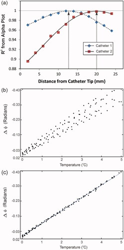
The MR-compatible heating array used for all hyperthermia experiments is shown in Figure 3(a). Figure 3(b) shows a fat-referenced PRFS temperature map with the general temperature sensor locations depicted in the image. As mentioned earlier, the sensor positions in a given catheter are fixed relative to one another. To prove that we have sensor–MRT coordinate registration, we start by assuming exact registration of the temperature probe filament tip and catheter tip, and therefore calculate the sensor locations starting from 0 mm along the spline. Given the high spatial resolution 3D fast-SPGR scans, the average offset error between fitted splines and the manually segmented catheter position is <0.25 mm. Therefore, if sensor localisation is correct, the PRFS phase change () for all sensors plotted as a function of reference temperature should yield a linear trend with a Pearson correlation (R²) of >0.995. In addition, the slope of the linear correlation provides a measure of the α-parameter. Figure 4(a) shows the R² correlation values for 2-mm increments for both temperature probes used in Figure 3(b). This plot indicates that the gross displacement for the temperature probe in catheter 1 is ∼13 mm, and the displacement for the temperature probe in catheter 2 is ∼20 mm. As the sensor points reach their true location along the spline, they coalesce to a single curve on the versus temperature plot, leading to an R² correlation >0.995 as indicated by the arrows in Figure 4(a). Figure 4(b) shows the versus temperature plot of all the sensors at the starting point of 0 mm along the spline. Figure 4(c) shows how the sensor plots merge into a single curve once the sensor positions are localised. The plot in Figure 4(c) shows versus temperature information for temperature probe sensors 1–3 localised at fixed relative positions of +13 mm along their corresponding spline fit, and for temperature probe sensors 4–6 localised at fixed relative positions of +20 mm along their corresponding spline fit. The slope of the curve in Figure 4(b) yields the α-parameter for the ‘gelatin’ phantom, α = 0.0123 ppm/°C, and is valid for all heating experiments using the same phantom material and imaging parameters. This value of α is high for water-based tissues, but falls within the range of literature values 0.0096–0.015 ppm/°C.

Figure 3. Heating array and axial MRT images. (a) MR-compatible heating array. The phantom sits inside a hollow water bolus cylinder. Patch hyperthermia antennas radiate phase-coherent RF at 434 MHz for heating. (b) Fat-referenced axial PRFS MRT map for slice 2 from Figure 2(a) showing general temperature probe sensor locations. Sensors 1–3 are part of one temperature probe for which the tip is located to the left of ‘3’. Sensors 4–6 are part of another temperature probe for which the tip is located to the right of ‘4’. Despite having four total sensor points per fibre-optic strand, during the experiments only three were usable, as one sensor was located in the fat/oil ring and therefore displayed no temperature-dependent phase change. The data for the sensor point located in the fat/oil is not shown.

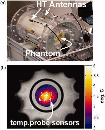
Figure 4. Sensor localisation and alpha calibration. (a) Shows the method used to determine temperature probe strand displacement inside each catheter. Each point on the plot represents the Pearson product-moment correlation (R²) of a linear regression line from a plot such as (b), where the PRFS phase change for all the sensors in a given catheter are plotted as a function of ground-truth temperature at a specific position along the spline curve. As you can see in (a), when the R² ∼ 1 (as indicated by the grey line) the temperature probes are localised correctly inside the catheters. Here the temperature probe in catheter 1 is shifted ∼13 mm, while the temperature probe in catheter 2 is shifted ∼20 mm as indicated by the arrows. (b) PRFS phase is shown as a function of ground-truth temperature for all sensors non-localised: i.e. assuming 0 mm difference in registration between the catheter and the temperature probe tips. Here R² < 0.900. (c) PRFS phase is shown as a function of ground-truth temperature for all sensors localised: i.e. after the sensors in temperature probe 1 have been shifted 13 mm and the sensors in temperature probe 2 have been shifted 20 mm from the catheter tip as indicated in (a). Here the R² > 0.998. The slope of this curve is the PRFS thermal coefficient (α-parameter).

Finally, to confirm the validity of our measurements of the ‘gelatin’ phantom temperature sensor locations and α, we repeated our experiments on the muscle-mimicking superstuff phantom. In that phantom, the α-parameter was found to be 0.0103 ppm/°C, which is more typical of water-based tissues.

Heating experiments

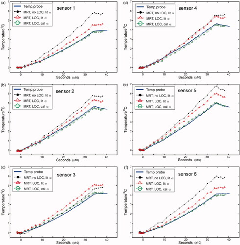
Heating experiments were performed to assess the accuracy of the methods presented in the MRT data registration section above. In each case, the difference between the MRT temperature and the sensor point temperature (ΔT) was used as the ultimate metric of accuracy. Figure 5 plots the temperature during the heating experiments as a function of time for all sensor points in the heating region. Atop the temperature probe data are MRT temperature plots for various processing conditions (See Figure 5 legend for details). The MRT data (green circles) plotted with the temperature probe data shows a virtually indistinguishable temperature plot. The improvement in this data compared to the other MRT data stems from the correctly localised temperature probe sensors and the resulting α-parameter calibration for this phantom material. The result corresponds to a reduced average error of ΔT < 0.14 °C with a maximum error of ΔT ∼ 0.22 °C. In contrast, the MRT data plotted without sensor localisation and using a nominal literature value of α = 0.010 ppm/°C yielded an average error of ΔT ∼ 1.42 °C with a maximum error of ΔT ∼ 2.21 °C (shown in Figure 5 as the solid black data points). We also note that using the correctly localised sensor positions and an assumed literature value of α = 0.010 ppm/°C yields an average error of ΔT ∼ 1 °C (Figure 5, red triangle points). To prevent over-fitting on a single data set, α values were only calculated once and used for other phantoms with the same material properties in different experiments. In addition, we confirmed the temperature probe shifts in the catheters by independent computed tomography (CT) measurements. Here, a wire of similar diameter to the temperature probe was inserted through the catheter. CT images clearly showed a gross displacement from the catheter tip for the 20-mm and 13-mm shifts mentioned above. MRT experiments were also performed with the superstuff phantom. These gave an average ΔT ∼ 0.2 °C, and overall trends that were consistent with the above findings for the gelatin phantom. In general, MRT accuracy is maximised when both sensor localisation and α calibration are addressed.

Figure 5. Heating experiments performed with ‘gelatin’ phantom. (a–f) The temperature data has been plotted for sensors 1–6 respectively, as depicted in Figure 3(b). On each plot, the ground-truth temperature data is represented by the solid blue curve. MRT data is also shown on each plot. Solid black circles represent MRT data processed for non-localised (no LOC) sensors assuming a literature PRFS-thermal coefficient (α-parameter) value of 0.01 ppm/°C (lit α). Hollow red triangle points represent MRT data processed for localised (LOC) sensors assuming a lit α. Hollow green circle points represent MRT data processed for localised (LOC) sensors with a calibrated α value of 0.0123 ppm/°C (cal α) from the slope of Figure 4(c). Similar results were obtained with the ‘superstuff’ phantom.

Discussion and conclusions

Although it is common practice to measure versus temperature to calculate the α-parameter [15,23,28], the use of multiple sensor points constrained to a catheter spline curve in a spatially localised heating pattern has not, to our knowledge, been employed in earlier work. The fitting of multiple independent sensor points at each sweeping step evaluates 3–4 different temperature evolutions making it possible to overcome MRT errors due to regional heating effects, e.g. a large temperature gradient. The use of a single sensor point along a non-linear catheter trajectory has many possible drawbacks. It may be difficult to locate – given no obvious fiducial point, and this puts further constraints on α calibration experiments as it would require very precise and uniform sample heating. Using the spline sweeping method for temperature sensor registration we can correct for errors in localising the temperature probe sensors and calibrate the material-specific α-parameter in a single experiment, without the necessity of slow uniform heating in the sample. Ultimately we have reduced these variables as a source of temperature probe/MRT data misregistration and presented a method that may be used as a benchmarking tool in any MRT validation application where invasive temperature probe placement is a routine practice.

Present experiments provide data showing the increased accuracy of MR thermometry data with fibre-optic reference temperature sensor data for two phantoms of distinct material properties. We found that for a non-linear catheter path, a 3D fast-SPGR sequence provides adequate contrast from which data points can be extracted, plotted, and fitted with cubic splines. These spline fits provide <0.25 mm error from catheter placement uncertainty and allow us to effectively localise multiple equi-spaced temperature sensors in MR coordinate space. We established the utility of carefully specifying the catheter tip in the spline curve from which we calculate the sensor locations. Most notably, if the temperature probe does not reach the catheter tip, the technique employs a positional sweep along the catheter path, where a plot of PRFS phase versus temperature is made at each positional increment. Ultimately, a Pearson correlation (R²) of >0.995 on the phase versus temperature plot indicates proper sensor localisation and α-parameter calibration. Given the linearity of our alpha plot data for multiple sensor points (R² of >0.995), and overall <0.5 degree Celsius discrepancy between reference probe and MRT calculation at equivalent time points, we can conclude that for the phantom materials and geometry, heating pattern and heating duration used in these experiments, there were no significant errors observed in our PRFS MRT readings from an electrical conductivity-induced phase-shift offset [35], or susceptibility-induced phase changes [36]. We note that in vivo any interface between materials of different susceptibility values may introduce a susceptibility artefact in the phase images, especially if the interface is perpendicular to the orientation of B₀. These may be problematic if they cannot be subtracted out to acquire a set of homogeneous steady-state temperature baseline images, e.g. if the susceptibility interface moves with time or if signal dephasing is severe enough to cause complete signal voids. Overall, conductivity-induced phase-shift offsets and/or susceptibility-induced phase changes may become more substantial as phantom heterogeneity, heating volume, heating uniformity, and heating duration are increased, and should therefore remain a topic of further investigation to mitigate PRFS MRT error for clinical hyperthermia applications.

The most critical impact of our results relates to the method presented, which provides the two-fold advantage of accurate sensor localisation and PRFS thermal coefficient (α) calibration. We have shown that this method is feasible and beneficial for MRT validation and α characterisation, i.e. only data paired with accurate probe localisation and α calibration yielded small errors between temperature probe and MRT during heating experiments. The techniques presented here may be used to simplify calibration experiments that use an interstitial heating device, or any heating method that provides rapid and spatially localised heat distributions, given that reference thermometry involves using multiple sensor points constrained along a catheter path. Overall, the experimental verification of the data registration and α calibration technique provides a useful benchmark method to maximise MRT accuracy in any similar context.

Declaration of interest

Matthew Tarasek, Lorne Hofstetter, Eric Fiveland, and Desmond Yeo are employees of GE Global Research and Gavin Houston is employed by GE Healthcare. The authors alone are responsible for the content and writing of the paper.

References

- Knavel EM, Brace CL. Tumor ablation: Common modalities and general practices. Tech Vasc Interv Radiol 2013;16:192–200
- van der Zee J. Heating the patient: A promising approach? Ann Oncol 2002;13:1173–84
- Kampinga HH. Cell biological effects of hyperthermia alone or combined with radiation or drugs: A short introduction to newcomers in the field. Int J Hyperthermia 2006;22:191–6
- Franckena M, van der Zee J. Use of combined radiation and hyperthermia for gynecological cancer. Curr Opin Obstet Gynecol 2010;22:9–14
- Issels RD, Lindner LH, Verweij J, Wust P, Reichardt P, Schem BC, et al. Neo-adjuvant chemotherapy alone or with regional hyperthermia for localised high-risk soft-tissue sarcoma: A randomised phase 3 multicentre study. Lancet Oncol 2010;11:561–70
- Vernon CC, Hand JW, Field SB, Machin D, Whaley JB, van der Zee J, et al. Radiotherapy with or without hyperthermia in the treatment of superficial localized breast cancer: Results from five randomized controlled trials. International Collaborative Hyperthermia Group. Int J Radiat Oncol Biol Phys 1996;35:731–44
- Hua Y, Ma S, Fu Z, Hu Q, Wang L, Piao Y. Intracavity hyperthermia in nasopharyngeal cancer: A phase III clinical study. Int J Hyperthermia 2011;27:180–6
- Huilgol NG, Gupta S, Sridhar CR. Hyperthermia with radiation in the treatment of locally advanced head and neck cancer: A report of randomized trial. J Cancer Res Ther 2010;6:492–6
- Valdagni R, Amichetti M. Report of long-term follow-up in a randomized trial comparing radiation therapy and radiation therapy plus hyperthermia to metastatic lymph nodes in stage IV head and neck patients. Int J Radiat Oncol Biol Phys 1994;28:163–9
- Paulides MM, Bakker JF, Linthorst M, van der Zee J, Rijnen Z, Neufeld E, et al. The clinical feasibility of deep hyperthermia treatment in the head and neck: New challenges for positioning and temperature measurement. Phys Med Biol 2010;55:2465–80
- Gellermann J, Wlodarczyk W, Ganter H, Nadobny J, Fahling H, Seebass M, et al. A practical approach to thermography in a hyperthermia/magnetic resonance hybrid system: Validation in a heterogeneous phantom. Int J Radiat Oncol Biol Phys 2005;61:267–77
- Kickhefel A, Rosenberg C, Weiss CR, Rempp H, Roland J, Schick F, et al. Clinical evaluation of MR temperature monitoring of laser-induced thermotherapy in human liver using the proton-resonance-frequency method and predictive models of cell death. J Magn Reson Imaging 2011;33:704–12
- Rieke V, Butts Pauly K. MR thermometry. J Magn Reson Imaging 2008;27:376–90
- van den Bosch M, Daniel B, Rieke V, Butts-Pauly K, Kermit E, Jeffrey S. MRI-guided radiofrequency ablation of breast cancer: Preliminary clinical experience. J Magn Reson Imaging 2008;27:204–8
- Weis J, Covaciu L, Rubertsson S, Allers M, Lunderquist A, Ahlstrom H. Noninvasive monitoring of brain temperature during mild hypothermia. Magn Reson Imaging 2009;27:923–32
- Wust P, Cho CH, Hildebrandt B, Gellermann J. Thermal monitoring: Invasive, minimal-invasive and non-invasive approaches. Int J Hyperthermia 2006;22:255–62
- Bloembergen N, Purcell EM, Pound RV. Relaxation effects in nuclear magnetic resonance absorption. Phys Rev 1948;73:679–712
- Parker DL. Applications of NMR imaging in hyperthermia: An evaluation of the potential for localized tissue heating and noninvasive temperature monitoring. IEEE Trans Biomed Eng 1984;31:161–7
- Bleier AR, Jolesz FA, Cohen MS, Weisskoff RM, Dalcanton JJ, Higuchi N, et al. Real-time magnetic resonance imaging of laser heat deposition in tissue. Magn Reson Med 1991;21:132–7
- Morvan D, Leroy-Willig A, Malgouyres A, Cuenod CA, Jehenson P, Syrota A. Simultaneous temperature and regional blood volume measurements in human muscle using an MRI fast diffusion technique. Magn Reson Med 1993;29:371–7
- De Poorter J, De Wagter C, De Deene Y, Thomsen C, Stahlberg F, Achten E. Noninvasive MRI thermometry with the proton resonance frequency (PRF) method: In vivo results in human muscle. Magn Reson Med 1995;33:74–81
- Ishihara Y, Calderon A, Watanabe H, Okamoto K, Suzuki Y, Kuroda K, et al. A precise and fast temperature mapping using water proton chemical shift. Magn Reson Med 1995;34:814–23
- Peters RD, Hinks RS, Henkelman RM. Ex vivo tissue-type independence in proton-resonance frequency shift MR thermometry. Magn Reson Med 1998;40:454–9
- Shrivastava D, Abosch A, Hughes J, Goerke U, DelaBarre L, Visaria R, et al. Heating induced near deep brain stimulation lead electrodes during magnetic resonance imaging with a 3 T transceive volume head coil. Phys Med Biol 2012;57:5651–65
- Soher BJ, Wyatt C, Reeder SB, MacFall JR. Noninvasive temperature mapping with MRI using chemical shift water–fat separation. Magn Reson Med 2010;63:1238–46
- Yung JP, Shetty A, Elliott A, Weinberg JS, McNichols RJ, Gowda A, et al. Quantitative comparison of thermal dose models in normal canine brain. Med Phys 2010;37:5313–21
- Pellicer R, Numan W, Tarasek MR, Hofstetter LW, Togni P, Bakker JF, et al. Rigorous investigation of muscle and fat mimicking phantom materials for MR-RF hyperthermia experiments. Paper presented at the European Society of Hyperthermic Oncology (ESHO) 28th Annual Meeting, Munich, Germany, 19–22 June 2013
- Yuan Y, Wyatt C, Maccarini P, Stauffer P, Craciunescu O, Macfall J, et al. A heterogeneous human tissue mimicking phantom for RF heating and MRI thermal monitoring verification. Phys Med Biol 2012;57:2021–37
- Paulides MM, Bakker JF, van Rhoon GC. Electromagnetic head-and-neck hyperthermia applicator: Experimental phantom verification and FDTD model. Int J Radiat Oncol Biol Phys 2007;68:612–20
- Hofstetter LW, Yeo DT, Dixon WT, Kempf JG, Davis CE, Foo TK. Fat-referenced MR thermometry in the breast and prostate using IDEAL. J Magn Reson Imaging 2012;36:722–32
- Kuroda K, Oshio K, Chung AH, Hynynen K, Jolesz FA. Temperature mapping using the water proton chemical shift: A chemical shift selective phase mapping method. Magn Reson Med 1997;38:845–51
- Shmatukha AV, Harvey PR, Bakker CJ. Correction of proton resonance frequency shift temperature maps for magnetic field disturbances using fat signal. J Magn Reson Imaging 2007;25:579–87
- Wyatt CR, Soher BJ, MacFall JR. Correction of breathing-induced errors in magnetic resonance thermometry of hyperthermia using multiecho field fitting techniques. Med Phys 2010;37:6300–9
- van der Zee J, van Rhoon GC, Broekmeijer-Reurink MP, Reinhold HS. The use of implanted closed-tip catheters for the introduction of thermometry probes during local hyperthermia treatment series. Int J Hyperthermia 1987;3:337–45
- Peters RD, Henkelman RM. Proton-resonance frequency shift MR thermometry is affected by changes in the electrical conductivity of tissue. Magn Reson Med 2000;43:62–71
- Sprinkhuizen SM, Konings MK, van der Bom MJ, Viergever MA, Bakker CJ, Bartels LW. Temperature-induced tissue susceptibility changes lead to significant temperature errors in PRFS-based MR thermometry during thermal interventions. Magn Reson Med 2010;64:1360–72