A model evaluation study for treatment planning of laser-induced thermal therapy

Abstract

A cross-validation analysis evaluating computer model prediction accuracy for a priori planning magnetic resonance-guided laser-induced thermal therapy (MRgLITT) procedures in treating focal diseased brain tissue is presented. Two mathematical models are considered. (1) A spectral element discretisation of the transient Pennes bioheat transfer equation is implemented to predict the laser-induced heating in perfused tissue. (2) A closed-form algorithm for predicting the steady-state heat transfer from a linear superposition of analytic point source heating functions is also considered. Prediction accuracy is retrospectively evaluated via leave-one-out cross-validation (LOOCV). Modelling predictions are quantitatively evaluated in terms of a Dice similarity coefficient (DSC) between the simulated thermal dose and thermal dose information contained within N = 22 MR thermometry datasets. During LOOCV analysis, the transient model’s DSC mean and median are 0.7323 and 0.8001 respectively, with 15 of 22 DSC values exceeding the success criterion of DSC ≥ 0.7. The steady-state model’s DSC mean and median are 0.6431 and 0.6770 respectively, with 10 of 22 passing. A one-sample, one-sided Wilcoxon signed-rank test indicates that the transient finite element method model achieves the prediction success criteria, DSC ≥ 0.7, at a statistically significant level.

• Bioheat transfer
• graphics processing unit (GPU)
• laser induced thermal therapy
• MR temperature imaging

Introduction

Approximately 211 000 patients in the USA present each year with brain tumours. Of these, 38 000 are benign primary tumours, 23 000 malignant primary tumours, and 150 000 are metastatic, originating largely from lung, breast, and melanoma [1–5]. The average life expectancy for patients with primary and metastatic malignancies in the brain, from time of diagnosis until death, is approximately 12–16 months. Five-year survival is among the lowest of all cancers. Current treatment options include conventional surgery, stereotactic radiosurgery (SRS), or chemotherapy. Surgical resection may be preferred for patients presenting with a single, solitary lesion, or lesions greater than 2.5–3.0 cm in which the size or location of the tumour causes neurological symptoms such as seizures, headaches, cognitive or motor deficits, that can be resolved by reducing the volume of the disease. SRS, such as Gamma Knife®, is typically performed on patients with multiple tumours, tumours under 2.5 cm in diameter, and deep seated tumours [6]. An additional target in the brain is epileptogenic foci for patients with medically refractory epilepsy, where MRgLITT is being considered for the surgical armamentarium for those patients [7,8]. Unfortunately, patients with malignant recurrences who have reached maximum radiation dose limitations and complications with surgical resection create a group of patients with no remaining conventional treatment options; meanwhile patients with medically refractory epilepsy have limited interventions available. Magnetic resonance-guided laser-induced thermal therapy (MRgLITT) presents an alternative, minimally invasive thermal ablation technique for these groups of patients and has been safely and successfully applied to each [9–15].

Under MR guidance, the laser applicator is carefully navigated through critical structures and placed directly into the diseased tissue to induce ablative heating and destroy the tissue. Real-time thermometry of the treatment volume during laser heating provides a mechanism by which it is possible to deliver these therapies in both a safe and effective manner [16–19] as well as to estimate the extent of tissue damage [20–22]. However, the heating induced by the laser is not constrained exclusively to tumour tissue and nearby tissue damage is possible. For these procedures to progress to standard of care, a priori determination of the optimal placement of the laser catheter(s) is crucial for achieving a more conformal delivery of therapy over the target volume with minimal co-morbidity of intervening or adjacent tissue. Surgical workflows in which the operating room and MRI suite are separate [7,23] escalate the advantages of a predictive model.

This manuscript focuses on the development of a practical methodology for evaluating computer model predictions for a priori planning the procedure, given N datasets from previous procedures. Evaluation focuses on prediction accuracy for guiding applicator placement. Retrospective analysis of MR thermometry data acquired during previous procedures is essential to train or calibrate the computer model parameters. The machine learning and statistics community have a rich history in applying various algorithmic and physics-based data models to reach conclusions from a given dataset [24,25]. Here we assume that a Pennes bioheat transfer model [26] provides representative predictions of the physical process underlying the heating observed within the MR thermometry data. This physics-based approach provides a theoretically sound and concise methodology to statistically summarise the high dimensional thermometry dataset with a low dimensional model parameter subset.

Two distinct modelling approaches are pursued: 1) A GPU implementation of an unstructured hexahedral spectral element method for predicting the bioheat transfer is developed, and 2) a computationally inexpensive algorithm for predicting the heat transfer from a linear superposition of analytic point source heating functions is also presented as a reference implementation. Combined with the data, the two modelling approaches presented provide an environment to critically evaluate model accuracy and selection for therapy planning of MRgLITT. Both approaches build intuition into the prediction by repetitively training the underlying physics model to statistically match representative datasets. Predictions are critically evaluated in terms of solution efficiency and accuracy for prospective treatment planning of MRgLITT procedures. Leave-one-out cross-validation (LOOCV) is used to simulate the clinical scenario in which N datasets from previous procedures are available to calibrate the computer model. LOOCV provides an objective framework to critically estimate the accuracy and confidence in predicting the outcome of the procedure for the N + 1 patient [27–31].

Methods

Thermometry data

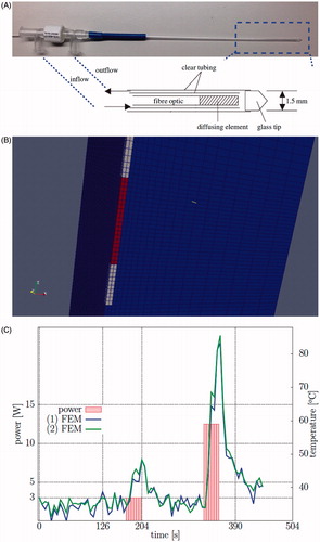
MR thermal monitoring from MRI-guided stereotactic laser-induced thermal therapy (LITT) was considered in N = 22 MR thermometry datasets. The datasets were vetted for motion artefacts, low signal-to-noise, and catheter-induced signal voids that spuriously reduce the modelling accuracy. Each patient was treated with the Visualase Thermal Therapy System (Visualase, Houston, TX). The Visualase® system includes a 15 W 980 nm diode laser, a cooling pump, and a laser applicator set. The laser applicator set is disposable and consists of a 400 μm core silica fibre optic with a cylindrical diffusing tip housed within a 1.65 mm diameter saline-cooled polycarbonate cooling catheter [12,22]; see Figure 1. Applicator cooling lines and laser fibre optics are connected through a waveguide between the control room and the bore of the MR magnet. An MR-compatible head holder is used to secure the patient’s head. The trajectory to the targeted tumour lesion was obtained using the Brainlab navigation system (Brainlab, Westchester, IL). A battery-powered hand drill was used to place a threaded plastic bone anchor within the skull. The laser applicator is secured to the threaded plastic bone anchor. The Visualase® system imports images from a 3D MPRAGE sequence to verify applicator position within the lesion. The depth is determined by the navigation software and is input retrospectively within this study.

Figure 1. (A) The Visualase® applicator modelled in this application and a diagram of the photon emitting diffusing tip and the cooling fluid are shown. (B) A finite element mesh conforms to the applicator and is used as the template for the calculations. (C) A representative time–temperature history profile is shown of the thermometry data at two points within the brain tissue, ∼1 mm from the applicator. The corresponding power history is also shown.

MR temperature imaging was performed on a 1.5 T MRI (GE Healthcare Technologies, Waukesha, WI) using a 2D gradient echo sequence [32] (flip angle = 30°, field of view = 24 × 24 cm², matrix size = 256 × 128, repetition time/echo time = 37.5/20 ms, receive-only head coil, 5 s per update). The imaging plane was chosen perpendicular to the axial direction of the applicator and allowed monitoring of critical structure regions. The Visualase® workstation communicates with the MR scanner to obtain raw DICOM imaging data during the procedure. The temperature-dependent water proton resonance frequency shift is measured by calculating the complex phase difference observed during heating. The water proton resonance frequency chemically shifts to lower frequencies with higher temperatures (caused by rupture, stretching, bending of hydrogen bonds) [33]. The total temperature change, Δu, is proportional to the measured phase change, δ φ.

Here α is the temperature sensitivity coefficient, γ is the gyromagnetic ratio of water, B₀ is the static magnetic field strength, and TE is the echo time. A baseline body temperature of u₀= 37.0 °C is assumed to obtain absolute temperature. An Arrhenius rate process model [34] was used to evaluate the thermal dose resulting from the time–temperature history of the laser exposure. (1)

In this Arrhenius thermal dose model, the frequency factor, A, and the activation energy, E_A, are experimentally determined kinetic parameters. The values for A and E_A were 3.1E98 s⁻¹ and 6.28E5 J mol⁻¹, respectively, and have been used in previous studies [9,35,36]. R is the universal gas constant. The thermal dose was assumed to be lethal at doses Ω ≥ 1 as seen in previous reports [9,36].

Prior to treatment delivery, a low power test pulse — e.g. 4 W for 30 s — is applied to verify the position of the diffusion fibre optic within the catheter. The test pulse is sufficient to allow thermal visualisation but not cause thermal damage. Multiple thermal imaging datasets are available per patient; only the therapeutic pulses are considered in this study. A representative laser power profile used during the therapy is shown in Figure 1. All DICOM header information was imported into an SQLite database to provide efficient queries and organise thermometry data for reproducible analysis and processing. The schema provided by the Slicer [37] DICOM module was used as a template for the table structure. The object identifier (OID) of the SQL table was used to provide anonymous references to the data. The SQL functions, ‘group by’, ‘group_concat’, and ‘count’, were used in quality assurance of the data location, number of files, for example. Metadata needed for the analysis included the following.

1. The applicator orientation and heating region of interest (ROI) were manually identified within the imaging datasets for input into the computer models discussed in the sections immediately below.

2. A text file containing the relevant laser power history for each imaging dataset was parsed and input into the simulation. The power history provides information on the heating and cooling time intervals during the procedure.

Simulation of bioheat transfer within laser irradiated tissue

A time-dependent Pennes [26] bioheat transfer equation provides a computer model for predicting the temperature field resulting from the laser tissue interaction. (2)

Here the tissue specific heat, c_p; tissue density, ρ; thermal conductivity, k; perfusion, ω; blood specific heat, c_blood; and arterial blood temperature, u_a, are deterministic model parameters obtained from the literature [38–40], see Table 1. The laser source, q_laser, is a deterministic function of the applied power, p(t); optical scattering, μ_s; optical absorption, μ_a; anisotropy factor, g; and distance, , from the source, U_tip. Active cooling of the water flowing through the applicator is modelled by a Robin or mixed boundary condition in which the temperature flux at the applicator interface is proportional to the convection coefficient, h, and the temperature difference between the cooling fluid u_cooling and the tissue. A diagram of the Visualase® applicator used in this application is shown in Figure 1.

Table 1. Constitutive data [38–40].

k		g [Unity]	μs [cm^−1]	μa [cm^−1]	ρ			h	ucooling [°C]	ua [°C]
0.527	9.0	0.88	14000	500	1045	3840	3600	100	21	37

An implicit Euler time discretisation is used to reduce the time-dependent bioheat equation, Equation 2(2) , into a sequence of elliptical problems. Hexahedral Lagrange elements (polynomial order = 3) were used in the finite element discretisation of the spatial domain. These elements use a tensor product of Gauss-Lobatto-Legendre (GLL) interpolation nodes and are commonly referred to as spectral elements. A matrix-free preconditioned conjugate gradient algorithm is used to solve the linear system of equations inherent inthe discretisation. An overlapping additive Schwarz preconditioner is used since the local block problem on each element is well suited for the block-coupled parallelism of the wide SIMD cores on the GPU. The matrix-free approach minimises the storage requirements and data movement of the finite element elliptical solvers. The preconditioned conjugate gradient algorithm does not explicitly demand the system matrix to be stored but only requires the evaluation of matrix vector products, and the structure of the tensor product hexahedral elements allow this action to be computed with O(N⁴) operations per degree-N finite element. Avoiding assembly and storage of the stiffness matrix on the GPU allows the solver to handle discretisations with a large number of elements to compensate for the limited memory on the GPU. This algorithmic approach is shown to have high computational efficiency on the non-uniform memory architecture of modern GPUs [41].

All computations were performed on the template hexahedral mesh shown in Figure 1(B). For each simulation the template was registered to the observed laser location for each patient. The mesh consists of disjoint regions for the applicator and tissue. A quadrilateral mesh was extruded axially along the applicator to create the base of the hexahedral finite element mesh. The mesh for the tissue conforms to the surface of the application and extends sufficiently far to ensure that the boundary does not influence the heating. The discretisation consists of N_dof = 844,032 total GLL nodes. The degrees of freedom across the volume of the applicator were removed; the effect of the room-temperature cooling fluid which protects the laser fibre during heating were considered through the boundary conditions at the surface nodes. Similar to previous studies [42], multiple mesh resolutions were considered to ensure convergence of the discretised solution; a mesh resolution approximating the 1 mm pixel size near the applicator was used. Multiple time resolutions were also evaluated to ensure convergence of the time stepping scheme.

Analytic steady-state solution

A steady-state version of the Pennes bioheat equation, Equation 2(2) , was also considered as a surrogate model for the therapy planning, in order to investigate the accuracy of a simpler, trained model. Constant coefficients are assumed. A one-dimensional spherically symmetrical radial decomposition of the solution, , simplifies the analysis of the differential operator in spherical coordinates.

From classical theory [43], the general solution is the linear combination of the homogeneous solution, u_h, and a particular solution, .

In this case, the particular solution was obtained from the method of undetermined coefficients for . (3)

The boundary conditions are used to determine the coefficients of the homogeneous solution. Applicator cooling is specified by the boundary condition at r = r₁ = 0.75 mm. The domain is assumed large enough that no heat flux is observed at the far boundary, r = r₂ = 1 m.

The one-dimensional solution provides an estimate of the heating from a single point source with applicator boundary at r₁. Mathematica 7 (Wolfram, Champaign, IL) was used to determine and verify all coefficients. Then, ccode was used to write out the kernel. Similar analytical solutions are provided in Giordano et al. [44–46]. Heating caused by the cylindrical geometry of the diffusing tip was modelled as evenly distributed point sources, M = 10, along the axial dimension of the applicator at positions . (4)

Model calibration

For each thermometry dataset discussed above, an inverse problem was solved to calibrate both computer models considered for the heating observed. Previous work [47] showed that the optical parameters provided the highest sensitivity in the temperature predictions over the range of physically meaningful model parameters. Consequently, optical parameters were considered in the optimisation. The analytical form of the standard diffusion approximation for the laser source term concisely represents the heating as a function of the single optical parameter, μ_eff. At the end of optimisation for one MRTI dataset, the dataset has a corresponding optimal μ_eff that is constant in space and time.

The out-of-plane translation component, z, of the mesh template shown in Figure 1 was also optimised. The physics of the MR thermometry data acquisition averages the temperature over the slice thickness and the translation update is implemented to tune the registration of the computational domain to the MR thermometry data. The remaining input parameters are assumed fixed.

The Dakota (Sandia National Laboratories, Albuquerque, NM) [48] library was used to optimise μ_eff for the transient and steady-state models. The L₂ error over space and time was used as the objective function. Thermometry data is denoted u^MRTI. All time steps were considered for the transient analysis of the computer model presented above. For the steady-state model presented above, the objective function was the L₂ norm between the model and the MRTI’s maximum heating time point. A quasi-Newton optimisation method, opp-q-newton, was implemented as the optimisation algorithm for both models. Gradients of the objective functions were computed using numerical finite differences. The calibration was solved as a bound constrained optimisation problem. A physically feasible parameter bound on the optimisation of the optical parameters, μ_eff ∈ (0.8, 400) m⁻¹, was obtained from the literature [39]. During calibration, the initial value for μ_eff was 180 m⁻¹. The initial value was calculated via the μ_eff identity from Equation 2(2) and the μ_a, μ_s, and g values from Table 1. The slice thickness of the MR thermometry data was used to bound the optimisation of the template out of plane translation.

Leave-one-out cross-validation

Leave-one-out cross-validation (LOOCV) is a method for estimating a trained, i.e. calibrated, model’s accuracy in prediction [27–31]. Within this context, developing a ‘predictive model’ refers to the process by which we can confidently assign a probability to a treatment outcome, such as full tumour destruction or damage to surrounding healthy tissue. Similar to the human cognitive process, the predictive computer model is built from prior experience using MR temperature imaging data used to monitor the procedure. The datasets are used to calibrate the computer model parameters as discussed in the previous section. The LOOCV algorithm is executed as:

• For each thermometry dataset i = 1, … , N.

• The average value for the optical coefficient, , is learned from the calibration results, , on the remaining j ≠ i datasets.

• Tissue damage on the i-th dataset is predicted by using the average, , values from the j ≠ i cohort. The Dice similarity coefficient (DSC) provides an estimate of the agreement with Arrhenius damage measured from thermometry data.

The DSC measures the area of overlap between the area enclosed by the Arrhenius damage model for the thermometry data, A, and the computer model prediction, B. The Arrhenius damage, Equation 1(1) , is computed from the simulated temperature field of the transient analysis. The isotherms are used as the damage model for the steady-state analysis. Previous work in canine brain demonstrated that the 57 °C isotherm produced damage regions similar to the Arrhenius model for the ablation regime considered in this study [49].

The trained model’s predictive ability is evaluated by analysing the distribution of DSC values from the N iterations of LOOCV. A one-sample, one-sided Wilcoxon signed rank test examines whether the trained model prediction’s median exceeds DSC ≥ 0.7. One-sample calculations were computed using a threshold DSC value, 0.7, as the null hypothesis H₀.

The value chosen is a commonly accepted value in image processing literature [49–51]; DSC = 1 implies complete agreement between the measure and predicted damage model, i.e. the predicted and measured damage volumes completely overlap. A two-sample, paired Wilcoxon signed-rank test was used to compare whether the two models’ prediction medians were statistically different from one another. All statistical tests and descriptive statistics were evaluated on GraphPad Prism 6.01 (GraphPad Software, La Jolla, CA).

Results

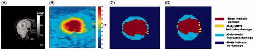
Representative thermometry images and calibrated computer model predictions are shown in Figure 2. The measured and predicted thermal dose is displayed. The Arrhenius damage model is shown for the transient model predictions, Equation 2(2) , and the thermometry data. The 57 °C isotherm damage model is shown for the steady-state analysis, Equation 4(4) . Significant variability is seen in the heating due to local patient tissue heterogeneities, tumour location, and nearby heat sinks in the brain such as large blood vessels and cerebral spinal fluid (CSF). This is reflected by the non-ellipsoidal shape of the isotherms and corresponding damage volume in the Arrhenius estimates of the damage. However, the calibrated thermal damage predictions show acceptable agreement, i.e. Dice similarity coefficient (DSC) ≥ 0.7 [51], between the measured and predicted tissue damage in multiple patients.

Figure 2. Representative thermometry data and calibrated model damage predictions. (A) The magnitude of the complex valued thermometry data provides a visualisation of the anatomy and is provided as a reference. The applicator trajectory is observed as a signal void in the image. The ROI displayed has a 3.75 × 3.28 cm² field of view and is shown in B–D. (B) MR thermometry at maximum heating is shown. (C) finite element method (FEM) model-predicted Arrhenius damage is compared to Arrhenius damage based on MRTI. (D) A comparison of the steady-state damage model is shown. The steady-state damage model is the region enclosed by the 57 °C isotherm. The colour map indicates the geometrical overlap used in DSC calculations; the legend is at right (C). Respective DSC values for the FEM model (C) and steady-state model (D) are DSC = 0.8385 and DSC = 0.7442.

The calibration process applied to each thermometry dataset provides a histogram of μ_eff values in which the optimal agreement between the model’s prediction and the MR thermometry is observed for each model. The histogram of the μ_eff values for both the transient and steady-state model calibrations is shown in Figure 3. Literature values of the expected optical properties are provided as a reference. Extrema of the feasible set are obtained from the range of values observed in the literature. Descriptive statistics of the optimised μ_eff values, DSC during optimisation, and DSC during LOOCV for both models is provided in Table 2; meanwhile, percentiles corresponding to interesting DSC thresholds are presented in Table 3.

Figure 3. Presented here are histograms of calibration analysis from the transient FEM model (A) and steady-state model (B), shown left and right, respectively. Both histograms have a bin width of 13.0 m⁻¹. The optical parameters, μ_eff, recovered from each thermometry dataset considered are shown. For each calibration the bound constrained optimisation was restricted to a range obtained from literature, μ_eff ∈ [0.8, 400] m⁻¹. Leave-one-out cross-validation was performed using these 22 μ_eff values. The nominal value in brain tissue obtained from Welch and van Gemert [39] is μ_eff = 180 m⁻¹.

Table 2. The descriptive statistics for μ_eff during optimisation and DSC performance during optimisation and LOOCV (N = 22). The transient solve of the Pennes bioheat equation using the Arrhenius damage, Equation 1(1) , is denoted by FEM. Steady-state analysis using the 57 °C isotherm damage model is denoted SS. Note that all DSC, skewness, and kurtosis quantities are unitless. %-ile refers to percentiles, e.g., 25%-ile means the dataset’s DSC performance exceeds 25% of the population DSC values in ranked order.

Descriptive statistic	FEM optimal μeff values (m^−1)	SS optimal μeff values (m^−1)	FEM optimal DSC values (Unity)	SS optimal DSC values (Unity)	FEM LOOCV DSC values (Unity)	SS LOOCV DSC values (Unity)
Minimum	67.26	138.4	0.4865	0.3421	0	0.3312
25%-ile	115.5	167.2	0.7356	0.5789	0.6709	0.5617
Median	121.6	189.6	0.8142	0.6925	0.8001	0.6770
75%-ile	146.1	212.4	0.8652	0.7259	0.8429	0.7257
Maximum	154.6	269.4	0.8972	0.8476	0.8859	0.8143
Mean	125.6	194.7	0.7824	0.6493	0.7323	0.6431
Standard deviation	21.78	38.42	0.1091	0.1274	0.1930	0.1289
Skewness	−0.7906	0.5714	−1.432	−1.190	−2.830	−1.150
Kurtosis	1.026	−0.2562	1.609	1.142	9.919	0.6817

FEM, finite element method; SS, steady state; opt., optimization; LOOCV, leave-one-out cross-validation; DSC, Dice similarity coefficient.

Table 3. The percentiles that correspond to several interesting DSC thresholds. The ‘opt.’ and ‘LOOCV’ columns refer to the same groups of datasets described in Table 2, as well as the datasets plotted in Figure 4. The smaller the percentile value, the better the model’s performance. ‘0’ indicates all values pass at the given threshold; ‘100’ indicates no values pass.

DSC threshold (Unity)	FEM (%-ile)	SS opt. (%-ile)	FEM (%-ile)	SS LOOCV (%-ile)
0.4	0	8.357	5.776	7.176
0.5	2.996	13.34	6.652	14.06
0.6	11.36	27.34	12.97	27.52
0.7	15.25	57.64	30.35	58.61
0.75	30.53	83.22	41.36	85.11
0.8	44.36	95.12	49.97	96.14
0.85	67.19	100	82.06	100

FEM, finite element method; SS, steady state; LOOCV, leave-one-out cross-validation; DSC, Dice similarity coefficient.

The overall DSC performance from both models during LOOCV analysis is provided in Figure 4. The performance is summarised by the number of datasets that pass a given DSC threshold; the plot is analogous to the Kaplan-Meier survival curve. During LOOCV, the transient model had 15 of 22 datasets pass the DSC ≥ 0.7 success criterion, while the steady-state model passed 10 of 22.

Figure 4. Here, the overall predictive performance, measured by DSC, is displayed for both models. (A) Left is the performance during optimisation, and (B) the right is during LOOCV. The horizontal axis displays increasing DSC thresholds; the vertical axis displays the number of datasets that pass the DSC threshold. Greater area under the curve (AUC) indicates better prediction. In the FEM LOOCV plot, there is one dataset that has a DSC = 0 and therefore does not appear on the plot.

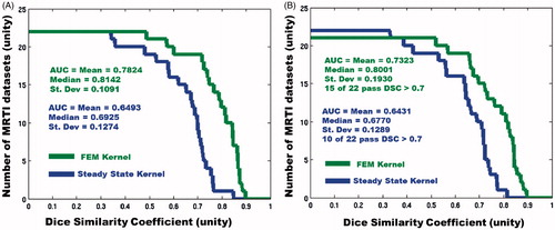
The two-sample, paired Wilcoxon signed-rank test rejected the null hypothesis with a p value of 0.0059; i.e. the difference of the transient and steady-state models’ medians of DSC during LOOCV was statistically significant. The one-sample, one-sided Wilcoxon signed-rank test for the transient model rejected the null hypothesis with a p value of 0.029; i.e. the transient model’s median of DSC during LOOCV was ≥0.7 at a statistically significant level. The one-sample, one-sided Wilcoxon signed-rank test for the steady-state model accepted the null hypothesis with a p value of 0.0732; i.e. the steady-state model’s median of DSC during LOOCV was not ≥0.7 at a statistically significant level.

Discussion

Given the number of available datasets, the LOOCV analysis provides a methodology to recapitulate the clinical scenario for treatment planning. Prior knowledge and experience is embodied within the thermometry data from the previous N ablations. Information from the previous ablations is extracted by calibrating a computer model to the available data. In this case, we calibrate our optical parameter to the thermometry data. Modelling goals are to ultimately utilise the calibrated model in optimising the thermal dose delivery. The success or failure of this paradigm is related to several factors. First, there must be a sufficient quantity of retrospective datasets for the training to converge. Second, the cohort of retrospective datasets used in training must have sufficient similarity within the group and to the prediction scenarios. Third, the model must be able to describe clinically relevant ablations.

If the LOOCV analysis only includes datasets that can be optimised to have DSC ≥ 0.7, both models perform very well. This is because the calibrated μ_eff values have a much tighter distribution; i.e. datasets with an optimal DSC ≥ 0.7 had similar μ_eff values. Given this investigation is framed as a prediction on the N + 1 patient, cherry-picking the successful optimisations is inappropriate. Indeed, optimisation results with DSC < 0.7 are included in the LOOCV analysis as seen in the descriptive statistics, Table 2. However, it is worth realising that successful optimisations have similar μ_eff values and perhaps information beyond the thermometry data would allow the calibration to be grouped into similar cohorts. For example additional meta information on the primary disease type, tumour location and treatment history would provide useful information in the analysis that may demonstrate clustering during the calibration and would further classify the tissue type.

The two models presented provide a canonical model selection comparison of the trade-off between the time investment in the algorithm, efficiency of the numerical implementation, and accuracy required for predicting the final endpoint of the application. The two-sided, two-sample paired Wilcoxon signed-rank test indicates the predictive results’ medians are significantly different and only the transient model’s median DSC performance was significantly ≥0.7. As a quantitative reference, the forward solve mapping between model parameters, Table 1, and temperature field is considered the fundamental computational operation of this study. Total run times in the analysis are proportional to the total number of forward solve iterations in the optimisation and LOOCV analysis. The run times for the forward solves in this study averaged 1.87E2 s and 1.12E1 s for the transient model GPU implementation and steady-state CPU implementation; respectively. These numbers are intended to provide intuition for the observed practical run times on a local CPU (Intel Xeon, 6 core, 2.4 GHz, double precision peak 57 Gflops) workstation with attach GPU accelerators (NVIDIA Tesla M2070 double precision peak 515 Gflops) available to this study. The finite element discretisation of the governing equations requires significant expertise of the GPU computing architecture as well as detailed algorithmic understanding of both the finite element technology and matrix-vector multiply within the iterative linear system solver to maximise floating point operation throughput and minimises memory transactions latencies. As opposed to explicitly storing and reading matrix entries from global memory, the matrix-free method recalculates the local matrix entries needed within the linear system solve. This memory access design pattern has demonstrated a 4–10× speed up over the matrix explicit methods [41,52,53]. Meanwhile, the steady-state superposition analysis, Equation 4(4) , provides treatment predictions with fewer floating point operations and would be selected under Occam’s razor [54] philosophy highly preferential to simplicity. While all kernels for the present spectral element methods and preconditioned conjugate gradient method were hand coded in this manuscript, library implementations of the matrix-free iterative solver approach are also appearing [53,55,56].

The finite element discretisation of the governing equations, however, provides significant opportunity for further physics-based improvements including higher order model spherical harmonic expansions in the laser fluence model [57]. As seen in Figure 3, the chosen models introduce a bias in the model parameter recovery that differs from published literature values. The bias may arise from inaccuracies in the modelling assumptions, perhaps most significant being the use of optical tissue properties that are invariant in space and time. The literature has clear examples where temperature/damage dependent and spatio-temporal dependent parameters are critical to the prediction [58,59]. The use of thermometry data during only the test pulse is also expected to influence the recovered optical properties. The choice to use a single constant parameter for full time history of each MRTI dataset is motivated by the practical model training focus of this investigation. Higher order physics models of the fluence are expected to provide the highest accuracy in recovering the optical parameters during the calibration process and for characterising the tissue properties.

The finite element discretisation of the governing equations also provides a rigorous physics-based methodology to incorporate tissue heterogeneities into the treatment prediction. Calibrations of the spatially heterogeneous optical parameter field have been shown to provide highly accurate predictions [60–62]. The inclusion of spatially varied, damage-dependent, and multiple parameters should be pursued in future efforts. Adjoint-based methods of computing the gradient of the objective function are necessary to efficiently optimise in the higher dimensional parameter space. Tissue heterogeneities could similarly be incorporated into the steady-state superposition analysis, Equation 4(4) , in a patient-specific ‘ad hoc’ manner. However, this would violate the underlying homogeneous tissue parameter assumptions which provided the mathematical structure for the concise analytical solution. A Gaussian process [63,64] framework may be appropriate in which the model parameters recovered may be interpreted as hyper-parameters for the covariance kernels. Similar to physics-based model calibration, optimisation of the hyper-parameters in the Gaussian process kernels offers a complementary trade-off between data fitting and smoothing. Further, Gaussian processes allow for prior information to be used and provide a full probabilistic prediction and an estimate of the uncertainty.

Model calibration and training was limited to thermometry data in these efforts. The predictive capabilities are expected to improve with more information provided by pre-treatment MR imaging such as dynamic contrast-enhanced imaging or perfusion imaging to help guide the selection of the model parameters, especially if these preoperative images can inform the optical parameters. Incorporating tissue heterogeneities into the model predictions would also require segmentations of the neuro-anatomy as a template for the regional heterogeneity. Each direction would benefit from the forethought of including these data acquisitions into the therapy protocol. For example, current brain segmentation techniques [65] require high resolution FLAIR, T2, and T1 imaging with and without contrast. The SQL database used in organising all data was vital to the reproducibility of the analysis in these efforts; this additional information must be incorporated. Tools for communicating with the neuro-navigation software to locate the fibre would also provide further information to improve the analysis throughput and reproducibility. Passive tracking of the applicator location using fiducials placed on the fibre would additionally provide the registration information needed to align the computational domain of the mathematical model.

Conclusion

Currently, the neurosurgeon reviews anatomical MR images to plan his/her trajectory to reach the tumour with neuro-navigation software, but does not have the capability to visualise outcomes of the laser ablation using various trajectories beforehand. Fully developed and commercially implemented predictive computer models will extend this functionality to include a priori visualisation and optimisation of the potential outcomes for complex treatment scenarios (multiple applicators/trajectories) in which the laser ablation is performed near a critical structure within a heterogeneous tissue environment. This work presents a step in this direction and demonstrates the feasibility in establishing a confidence in these predictions. Consideration of other available metadata to improve prediction accuracy is a topic of on-going research.

Acknowledgements

The authors would like to thank Roger McNichols, PhD, for his assistance in clinical laser ablation as well as the DAKOTA [48], ITK [66], Paraview [67], and CUBIT [68] communities for providing enabling software for scientific computation and visualisation.

Declaration of interest

The research in this paper was supported in part through grants from the O’Donnell Foundation, US National Science Foundation AIR-1312048, US National Institutes of Health 1R21EB01016-01, National Center for Advancing Translational Sciences of the National Institutes of Health TL1TR000369, US Department of Defence W81XWH-14-1-0024, and the Cancer Center Support Grants CA016672 and CA79282. Research was jointly conducted at the MD Anderson Center for Advanced Biomedical Imaging in part with equipment support from General Electric Healthcare. At the time of this work, Visualase, Inc. and BioTex, Inc. provided the surgical device technology and services. Anil Shetty and Ashok Gowda were employed by those companies. Since that time, Medtronic, Inc. has acquired Visualase, Inc., and employs Anil Shetty. BioTex, Inc. employs Ashok Gowda. Shabbar Danish has received educational honoraria from Medtronic, Inc. The authors alone are responsible for the content and writing of the paper.

References

- Siegel R, Naishadham D, Jemal A. Cancer statistics, 2013. CA Cancer J Clin 2013;63:11–30
- Kalkanis SN, Linskey ME. Evidence-based clinical practice parameter guidelines for the treatment of patients with metastatic brain tumors: Introduction. J Neurooncol 2010;96:7–10
- Gavrilovic IT, Posner JB. Brain metastases: Epidemiology and pathophysiology. J Neurooncol 2005;75:5–14
- Bafaloukos D, Gogas H. The treatment of brain metastases in melanoma patients. Cancer Treat Rev 2004;30:515–20
- Owonikoko TK, Arbiser J, Zelnak A, Shu H-KG, Shim H, Robin AM, et al. Current approaches to the treatment of metastatic brain tumours. Nat Rev Clin Oncol 2014;11:203–22
- Alexander E, Moriarty TM, Davis RB, Wen PY, Fine HA, Black PM, et al. Stereotactic radiosurgery for the definitive, noninvasive treatment of brain metastases. J Natl Cancer Inst 1995;87:34–40
- Curry DJ, Gowda A, McNichols RJ, Wilfong AA. MR-guided stereotactic laser ablation of epileptogenic foci in children. Epilepsy Behav 2012;24:408–14
- Nowell M, Miserocchi A, McEvoy AW, Duncan JS. Advances in epilepsy surgery. J Neurol Neurosurg Psychiatry 2014;85:1273–9
- Carpentier A, Itzcovitz J, Payen D, George B, McNichols RJ, Gowda A, et al. Real-time magnetic resonance-guided laser thermal therapy for focal metastatic brain tumors. Neurosurgery 2008;63:ONS21–9
- Carpentier A, McNichols RJ, Stafford RJ, Guichard J-P, Reizine D, Delaloge S, et al. Laser thermal therapy: Real-time MRI-guided and computer-controlled procedures for metastatic brain tumors. Lasers Surg Med 2011;43:943–50
- Carpentier A, Chauvet D, Reina V, Beccaria K, Leclerq D, McNichols RJ, et al. MR-guided LITT for recurrent glioblastomas. Lasers Surg Med 2012;44:361–8
- Torres-Reveron J, Tomasiewicz HC, Shetty A, Amankulor NM, Chiang VL. Stereotactic laser induced thermotherapy (LITT): A novel treatment for brain lesions regrowing after radiosurgery. J Neurooncol 2013;113:495–503
- Jethwa PR, Barrese JC, Gowda A, Shetty A, Danish SF. Magnetic resonance thermometry-guided laser-induced thermal therapy for intracranial neoplasms: Initial experience. Neurosurgery 2012;71:ons133–45
- Schwarzmaier H-J, Eickmeyer F, Fiedler VU, Ulrich F. Basic principles of laser induced interstitial thermotherapy in brain tumors. Med Laser Appl 2002;17:147–58
- Schulze PC, Vitzthum HE, Goldammer A, Schneider JP, Schober R. Laser-induced thermotherapy of neoplastic lesions in the brain – underlying tissue alterations, MRI-monitoring and clinical applicability. Acta Neurochir (Wien) 2004;146:803–12
- Rieke V, Butts Pauly K. MR thermometry. J Magn Reson Imaging 2008;27:376–90
- De Senneville BD, Quesson B, Moonen CTW. Magnetic resonance temperature imaging. Int J Hyperthermia 2005;21:515–31
- Stafford RJ, Shetty A, Elliott AM, Klumpp SA, McNichols RJ, Gowda A, et al. Magnetic resonance guided, focal laser induced interstitial thermal therapy in a canine prostate model. J Urol 2010;184:1514–20
- Woodrum DA, Gorny KR, Mynderse LA, Amrami KK, Felmlee JP, Bjarnason H, et al. Feasibility of 3.0 T magnetic resonance imaging-guided laser ablation of a cadaveric prostate. Urology 2010;75:1514.e1–6
- Dewhirst MW, Viglianti BL, Lora-Michiels M, Hanson M, Hoopes PJ. Basic principles of thermal dosimetry and thermal thresholds for tissue damage from hyperthermia. Int J Hyperthermia 2003;19:267–94
- McDannold N, Tempany CM, Fennessy FM, So MJ, Rybicki FJ, Stewart EA, et al. Uterine leiomyomas: MR imaging-based thermometry and thermal dosimetry during focused ultrasound thermal ablation. Radiology 2006;240:263–72
- McNichols RJ, Kangasniemi M, Gowda A, Bankson JA, Price RE, Hazle JD. Technical developments for cerebral thermal treatment: Water-cooled diffusing laser fibre tips and temperature-sensitive MRI using intersecting image planes. Int J Hyperthermia 2004;20:45–56
- Tovar-Spinoza Z, Carter D, Ferrone D, Eksioglu Y, Huckins S. The use of MRI-guided laser-induced thermal ablation for epilepsy. Child’s Nerv Syst 2013;29:2089–94
- Breiman L. Statistical modeling: The two cultures (with comments and a rejoinder by the author). Stat Sci 2001;16:199–231
- Hastie T, Tibshirani R, Friedman J. The elements of statistical learning: Data mining, inference and prediction. Math Intell 2005;27:83–5
- Pennes HH. Analysis of tissue and arterial blood temperatures in the resting human forearm. J Appl Physiol 1948;1:1725–32
- Stone M. Cross-validatory choice and assessment of statistical predictions. J R Stat Soc Ser B 1974;36:111–47
- Geisser S. The predictive sample reuse method with applications. J Am Stat Assoc 1975;70:320–8
- Kohavi R. A study of cross-validation and bootstrap for accuracy estimation and model selection. Proc 14th Int Jt Conf Artif Intell San Francisco, CA 1995;1137–43
- Browne M. Cross-validation methods. J Math Psychol 2000;44:108–32
- Arlot S, Celisse A. A survey of cross-validation procedures for model selection. Stat Surv 2010;4:40–79
- Stafford RJ, Price RE, Diederich CJ, Kangasniemi M, Olsson LE, Hazle JD. Interleaved echo-planar imaging for fast multiplanar magnetic resonance temperature imaging of ultrasound thermal ablation therapy. J Magn Reson Imaging 2004;20:706–14
- Ishihara Y, Calderon A, Watanabe H, Okamoto K, Suzuki Y, Kuroda K, et al. A precise and fast temperature mapping using water proton chemical shift. Magn Reson Med 1995;34:814–23
- Pearce J, Thomsen S. Rate process analysis of thermal damage. In: Welch AJ, Gemert MJC Van, editors. Optical-Thermal Response of Laser-Irradiated Tissue. New York: Springer; 1995. pp. 561–606
- Schwarzmaier HJ, Yaroslavsky I V, Yaroslavsky a N, Fiedler V, Ulrich F, Kahn T. Treatment planning for MRI-guided laser-induced interstitial thermotherapy of brain tumors – the role of blood perfusion. J Magn Reson Imaging 1998;8:121–7
- McNichols RJ, Gowda A, Kangasniemi M, Bankson JA, Price RE, Hazle JD. MR thermometry-based feedback control of laser interstitial thermal therapy at 980 nm. Lasers Surg Med 2004;34:48–55
- Yeniaras E, Fuentes DT, Fahrenholtz SJ, Weinberg JS, Maier F, Hazle JD, et al. Design and initial evaluation of a treatment planning software system for MRI-guided laser ablation in the brain. Int J Comput Assist Radiol Surg 2013;9:659–67
- Diller KR, Valvano JW, Pearce JA. Bioheat transfer. In: Kreith F, Goswami Y, eds. CRC Handbook of Mechanical Engineering, 2nd ed. Boca Raton: CRC Press, 2005. pp. 4--114 to 4--215
- Welch AJ, van Gemert MJC. Optical-Thermal Response of Laser-Irradiated Tissue. 2nd ed. New York: Springer; 2010
- Duck FA. Physical Properties of Tissue: A Comprehensive Reference Book. London: Academic Press; 1990
- Medina DS, St-Cyr A, Warburton T. OCCA: A unified approach to multi-threading languages. arXiv 2014;1403.0968v1:1–25
- Fuentes D, Walker C, Elliott A, Shetty A, Hazle JD, Stafford RJ. Magnetic resonance temperature imaging validation of a bioheat transfer model for laser-induced thermal therapy. Int J Hyperthermia 2011;27:453–64
- Boyce WE, Diprima RC, Haines CW. Elementary Differential Equations and Boundary Value Problems. 7th ed. New York: Wiley; 2001
- Giordano MA, Gutierrez G, Rinaldi C. Fundamental solutions to the bioheat equation and their application to magnetic fluid hyperthermia. Int J Hyperthermia 2010;26:475–84
- Vyas R, Rustgi ML. Green’s function solution to the tissue bioheat equation. Med Phys 1992;19:1319–24
- Deng Z-S, Liu J. Analytical study on bioheat transfer broblems with spatial or transient heating on skin surface or inside biological bodies. J Biomech Eng 2002;124:638--49
- Fahrenholtz SJ, Stafford RJ, Maier F, Hazle JD, Fuentes D. Generalised polynomial chaos-based uncertainty quantification for planning MRgLITT procedures. Int J Hyperthermia 2013;29:324–35
- Eldred MS, Giunta AA, van Bloemen Waanders BG, Wojtkiewicz SF, Hart WE, Alleva MP. DAKOTA, a Multilevel Parallel Object-Oriented Framework for Design Optimization, Parameter Estimation, Uncertainty Quantification, and Sensitivity Analysis: Version 4.1 Reference Manual. Albuquerque, NM: Sandia National Laboratories; 2007
- Yung JP, Shetty A, Elliott A, Weinberg JS, McNichols RJ, Gowda A, et al. Quantitative comparison of thermal dose models in normal canine brain. Med Phys 2010;37:5313–21
- Dice LR. Measures of the amount of ecologic association between species. Ecol Soc Am 1945;26:297–302
- Zou KH, Wells WM, Kikinis R, Warfield SK. Three validation metrics for automated probabilistic image segmentation of brain tumours. Stat Med 2004;23:1259–82
- Mueller E, Guo X, Scheichl R, Shi S. Matrix-free GPU implementation of a preconditioned conjugate gradient solver for anisotropic elliptic PDEs. Comput Vis Sci 2013;16:41–58
- Knepley MG, Terrel AR. Finite element integration on GPUs. ACM Trans Math Softw 2013;39:1–13
- Jaynes ET, Bretthorst GL. Probability Theory: The Logic of Science. Cambridge: Cambridge University Press; 2003
- Knepley MG, Brown J, Rupp K, Smith BF. Achieving high performance with unified residual evaluation. arXiv 2013;1309.1204v2:4
- Knepley MG, Kupp K, Terrel AR. Finite element integration with quadrature on accelerators. ACM Trans Math Softw 2015
- Carp SA, Prahl SA, Venugopalan V. Radiative transport in the delta-P1 approximation: Accuracy of fluence rate and optical penetration depth predictions in turbid semi-infinite media. J Biomed Opt 2004;9:632–47
- Mohammed Y, Verhey JF. A finite element method model to simulate laser interstitial thermo therapy in anatomical inhomogeneous regions. Biomed Eng Online 2005;4:2
- Schutt DJ, Haemmerich D. Effects of variation in perfusion rates and of perfusion models in computational models of radio frequency tumor ablation. Med Phys 2008;35:3462
- Fuentes D, Elliott A, Weinberg JS, Shetty A, Hazle JD, Stafford RJ. An inverse problem approach to recovery of in vivo nanoparticle concentrations from thermal image monitoring of MR-guided laser induced thermal therapy. Ann Biomed Eng 2012;41:100–11
- Diller KR, Oden JT, Bajaj C, Browne JC, Hazle JD, Babuška I, et al. Computational infrastructure for the real-time patient-specific treatment of cancer. In: Minkowycz WJ, Sparrow EM, editors. Advances in Numerical Heat Transfer: Numerical Implementation of Bioheat Models and Equations. Vol. 3. New York: Taylor and Francis; 2009. pp. 307--344
- Feng Y, Fuentes D, Hawkins A, Bass JM, Rylander MN. Optimization and real-time control for laser treatment of heterogeneous soft tissues. Comput Methods Appl Mech Eng 2009;198:1742–50
- Rasmussen CE, Williams CKI. Gaussian Processes for Machine Learning. Cambridge, MA, USA: MIT Press; 2006
- Constantinescu EM, Anitescu M. Physics-based covariance models for Gaussian processes with multiple outputs. Int J Uncertain Quantif 2013;3:47--71
- Menze B, Jakab A, Bauer S, Kalpathy-Cramer J, Farahani K, Kirby J, et al. The Multimodal Brain Tumor Image Segmentation Benchmark (BRATS). IEEE Trans Med Imaging 2014;2014:1–32
- Ibanez L, Schroeder W, Ng L, Cates J. The ITK Software Guide. Clifton Park, NY, USA: Kitware; 2005
- Henderson A, Ahrens J. The ParaView Guide: A Parallel Visualization Application. Clifton Park, NY: Kitware; 2004
- Blacker TD, Bohnhoff W, Edwards T. CUBIT Mesh Generation Environment.Volume 1: Users Manual. Albuquerque, NM: Sandia National Laboratories; 2004