Registering 2D and 3D imaging data of bone during healing

Abstract

Purpose/Aims of the study: Bone’s hierarchical structure can be visualized using a variety of methods. Many techniques, such as light and electron microscopy generate two-dimensional (2D) images, while micro-computed tomography (µCT) allows a direct representation of the three-dimensional (3D) structure. In addition, different methods provide complementary structural information, such as the arrangement of organic or inorganic compounds. The overall aim of the present study is to answer bone research questions by linking information of different 2D and 3D imaging techniques. A great challenge in combining different methods arises from the fact that they usually reflect different characteristics of the real structure.

Materials and methods: We investigated bone during healing by means of µCT and a couple of 2D methods. Backscattered electron images were used to qualitatively evaluate the tissue’s calcium content and served as a position map for other experimental data. Nanoindentation and X-ray scattering experiments were performed to visualize mechanical and structural properties.

Results: We present an approach for the registration of 2D data in a 3D µCT reference frame, where scanning electron microscopies serve as a methodic link. Backscattered electron images are perfectly suited for registration into µCT reference frames, since both show structures based on the same physical principles. We introduce specific registration tools that have been developed to perform the registration process in a semi-automatic way.

Conclusions: By applying this routine, we were able to exactly locate structural information (e.g. mineral particle properties) in the 3D bone volume. In bone healing studies this will help to better understand basic formation, remodeling and mineralization processes.

• Backscattered electron imaging
• micro-computed tomography
• semi-automatic image registration
• three-dimensional visualization

Introduction

In bone research, there is an increasing demand to track temporal and spatial changes in bone material properties during healing and adaptation processes. Combining information representing different structural and functional properties of bone and visualizing them together helps to understand these processes. To obtain this structural and functional information, not only different image modalities are used, but the imaging techniques also operate on different length scales. While for some aspects three-dimensional (3D) images are acquired, other properties are only obtained in a two-dimensional (2D) plane. Integration of these different types of datasets usually requires some kind of registration process.

It is well known that bone has different functions within the organism, such as enabling locomotion and serving as a mineral reservoir (1). To maintain or restore its functionality, it has a great adaptive and regenerative potential in response to mechanical loads or after injuries. Bone undergoes different stages of healing (2) through which the bone structure changes remarkably. During bony callus formation, primary bone material is usually quickly deposited in a first wave and replaced by highly structured lamellar bone in a second wave (3). To elucidate bone’s adaptation and regeneration processes, it is crucial to investigate bone from different perspectives with a variety of complementary methods. In addition to biological techniques and tools, which reveal histological, biochemical, genetic and cellular information, several methods enable a visualization of structural, physical and mechanical properties at different length scales.

From a materials science perspective, bone is regarded as a nanocomposite material consisting of hydroxyapatite platelets within a collagen matrix (4,5). It has extraordinary structural properties, since it consists of different hierarchical levels and all these levels reveal changes during fracture healing (6). These changes in material properties are investigated in a spatially and temporally resolved way using various methods. Microscopy methods give information on the micrometer level, for example, polarized light microscopy visualizes the orientation of collagen fibrils and confocal laser scanning microscopy reveals the osteocyte network (7). Scanning electron microscopy (SEM) detecting backscattered electrons (BSE) qualitatively shows the mineral content within the bony tissue (8). Using nanoindentation, hardness and indentation modulus are calculated (9). With X-ray scattering techniques, also including synchrotron experiments, information on the nanometer level is collected. The mean thickness, the degree of alignment and the predominant orientation of the mineral particles are determined (10). Combining these multiple methods helps to understand the healing progress with the changing structural and functional characteristics of the bone material. However, all these methods are performed in 2D planes and their results are generally only visualized as such.

Since bone has a 3D structure, investigations of processes in bone should also consider its 3D nature. Micro-computed tomography (µCT) is used to examine bone samples in 3D (Figure 1A). During tomography scanning, the X-ray beam becomes more attenuated as it passes through the thicker, denser portions of the bone material. Thus, it is possible to reconstruct a highly detailed 3D model, where even fine trabeculae within the bone are non-destructively visualized (11). The attenuation of the X-rays is reported to be proportional to the tissue density (12). Therefore, not only mineralized and non-mineralized tissue parts are distinguishable, but also the degree of mineralization of the bone material is qualitatively shown by the resulting gray values. Even more important, µCT data can be used as a reference frame to incorporate 2D datasets from other methods using the environmental scanning electron microscopy in backscattered electron mode (ESEM/BSE) as methodic link. The ESEM/BSE images exhibit two essential properties to serve as reference for other 2D methods and to find the exact location of the 2D plane in a 3D µCT dataset: (i) They are produced in high resolution relatively fast, so that on the one hand their resolution corresponds to the resolution of the characterizing methods and on the other hand they visualize large parts of the analyzed structure or even the whole bone. (ii) They are perfectly suited for semi-automatic registration into the µCT datasets since they equally translate the mineral content into different gray values and show structures that are visible in 2D sections of the µCT models in an identical way (Figure 1C–E).

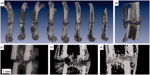
Figure 1. Two typical datasets for 2D-3D registration. Panel A shows a volume rendering of a µCT dataset visualizing a 3D model of an osteotomized rat femur with a non-critical-size osteotomy, four weeks post-osteotomy. The complete bone is rotated around the major axis and shown from different sides. Furthermore, the bone is intersected at different levels to see the inner structure. Panel B gives a higher resolved µCT scan of the osteotomy. In panel B, the bony periosteal and endosteal callus tissue is clearly detected. Panels C to E are environmental scanning electron microscopy images in backscattered electron mode (ESEM/BSE) of non-critical-size femoral osteotomies in rats at three, four, and six weeks post-osteotomy.

Both ESEM/BSE and µCT can also be performed in a quantitative manner using calibrated systems to describe the mineral density of the bone (8,13). Thereby, different gray values correspond directly to values of the bone mineral content. Using either ESEM/BSE or µCT in a quantitative way would enable to evaluate the differences of the qualitative values of the other method to exact quantitative values.

Generally, the need to progress in automatic image registration, i.e. in overlaying images by geometric transformations, increases in general with the growing diversity of imaging methods and the amount of image data produced (14). A good overview of image registration methods can be found, for example, in the surveys of Zitova et al. (14) and Pluim et al. (15) as well as in the monographs of Goshtasby (16) and Modersitzki (17). In the present study, registering the experimental data within a 3D reference frame is realized in a two-step process: (I) Manual registration of the experimental results into ESEM/BSE images. Performing these characterizing experiments is usually very time-consuming. The measurements are generally in high resolution and therefore restricted to small areas. (II) Semi-automatic integration of the ESEM/BSE images into the µCT models (following the schematic description in Figure 3, see Figure 2 as an example) and repeat this integrating transformation with the experimental results.

Figure 2. 3D localization of backscattered electron (ESEM/BSE) image plane within the 3D µCT dataset. Panel A shows an ESEM/BSE image of a rat femoral osteotomy, four weeks post-osteotomy. Panel B gives a slice of a virtual section through a µCT volume rendering at the site of the exact location of the ESEM/BSE image and C the same view where the volume is cut in half by this plane. Panels D and E visualize the 3D position of the section within the µCT reference dataset, locally and within the whole bone.

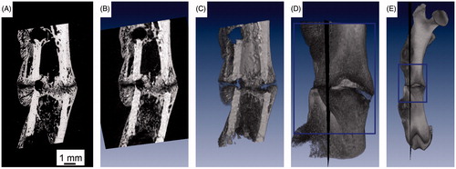
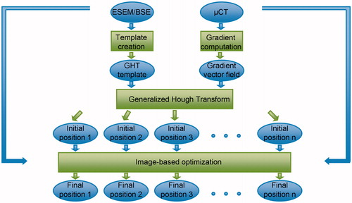
Figure 3. Schematic description of the different steps of the registration process. The backscattered electron (ESEM/BSE) image and the µCT dataset are used to determine a template and a gradient vector field, respectively, for the GHT. The GHT is then used to calculate n different initial positions that are stored and optimized using an image-based fine registration process resulting in n final positions.

In this study, we show how crucial it is to take into account the 3D position of characterizing measurements, such as nanoindentation or X-ray scattering, to correctly interpret the data. It is essential to know whether the section where the measurement was performed is tilted with respect to the major axis of the bone and if it is at the side of the bone rather than in the center (Figure 2). We present a workflow and techniques that allow us to integrate 2D information into a 3D µCT volume. We use ESEM/BSE images as methodic link, since these exhibit similar image properties as the µCT image. Our workflow was specifically designed to handle the challenging case where the 2D image (ESEM/BSE) resembles a large number of slices with different positions and orientations in the 3D image. In our datasets, this was due to the rotational symmetry around the major axis of the bone. As a result, many local optima appear in the objective function, making the registration process a demanding task. The problem of integrating 2D image slices into 3D image volumes has been the subject of a few recent publications including the ones by Osechinskiy and Kruggel (18) and Ferrante and Paragios (19). However, to the best of our knowledge, none of these works handles the problem of determining initial starting positions for the local optimization procedure. Due to the high degree of rotational symmetry, manually determining this initial position, as was done in the previously mentioned publications (18,19), is infeasible. We therefore propose to use the generalized Hough transform (GHT) (20) for identifying suitable starting positions and show that this seems to be suitable for µCT and ESEM/BSE images. In the following, we present methods together with a work flow to quickly register 2D and 3D datasets in a semi-automatic way as well as to visualize structures and properties of bone during healing.

Materials and methods

Sample preparation

Developing and testing of the software was performed using datasets derived from rat femoral osteotomy samples.

Surgical procedure

Non-critical (1 mm, see Figure 1C–E) and critical-size (5 mm, see Figure S1) osteotomies were produced following the operative procedure described previously (21,22). Briefly, the animals (female Sprague-Dawley rats, 12 weeks old, 250 g to 300 g) were anesthetized with ketamine hydrochloride (60 mg/kg, Ketamine 50 mg, Actavis Group, Hafnarfjördur, Iceland) and medetomidine (0.3 mg/kg, Domitor®, Pfizer, Karlsruhe, Germany) and treated with an antibiotic (clindamycin-2-dihydrogenphosphate 45 mg/kg, Ratiopharm, Ulm, Germany). In the midshaft of the femur, an osteotomy was created using an oscillating saw and an external fixator with four pins was used to stabilize the osteotomy. An analgesic (tramadol hydrochloride, Grünenthal, Aachen, Germany) was given during the surgery and during the following three days. The animals were sacrificed two, three, four or six weeks after surgery. All animal experiments were in accordance to the policies and procedures of the local legal representative (LAGeSo Berlin, G0071/07).

Further sample processing

After scanning the samples with a µCT (described later in the section “Micro-computed tomography”), further sample preparation steps, such as embedding, cutting and grinding were performed as previously specified (23). Briefly, the samples were fixed in 10% formalin. For dehydration, they were put in ascending concentrations of ethanol and finally they were put in Xylol. PMMA-embedding was performed using methylmethacrylate (MMA, Technovit® 9100 new, Heraeus Kulzer GmbH, Wehrheim, Germany). The samples were cut using a low-speed diamond saw (Buehler Isomet, Buehler GmbH, Duesseldorf, Germany) and ground by hand with 1200 silicon carbide grinding paper (grain size 15 µm). ESEM/BSE images (see section “Environmental scanning electron microscopy in backscattered electron mode”) and other experiments (see section “Experimental methods for 2D data for integration into 3D datasets”) were then performed using blocks or thin slices of the embedded samples with ground and polished surfaces.

Micro-computed tomography

Micro-computed tomography of freshly harvested osteotomized rat femurs was performed with a µCT scanner (viva40, Scanco Medical, Brüttisellen, Switzerland) at a voltage of 70 kV, an intensity of 114 µA, 600 ms integration time and no frame averaging. Micro-computed tomograms of the midshaft regions, including the osteotomy site and the area with newly formed callus tissue were acquired at a 28-fold magnification. The reconstructed 3D datasets had a voxel size of 10.5 µm × 10.5 µm × 10.5 µm. A sub-set of samples was scanned within ethanol with a SkyScan1072 µCT scanner (SkyScan, Aartselaar, Belgium). The measurement was performed using a 1 mm Al filter at a voltage of 80 kV and an intensity of 98 µA during an integration time of 6 s. We scanned again the midshaft region with the osteotomy and the callus structure with a magnification of 28.2 resulting in a voxel size of 10.3 µm × 10.3 µm × 10.3 µm (Figure 1B). Additionally, we made bigger scans of the whole bone for selected samples with a magnification of 15.6 and a voxel size of 18.7 µm × 18.7 µm × 18.7 µm (Figure 1A). Collecting radiographic projections at different angles led to a 3D dataset with different gray values. The gray value of every voxel reflects the mineral content as the attenuation is proportional to the density of the irradiated sample volume (12).

The two different scanners resulted in totally different ranges of gray value that correspond to the mineral density within the bone.

Environmental scanning electron microscopy in backscattered electron mode

To produce the BSE images, we used blocks or thin slices of PMMA-embedded samples with ground surfaces. The setup consisted of an environmental scanning electron microscope (ESEM, Quanta 600, FEI, Hillsboro, OR) equipped with a backscattered electron detector under the following conditions: working distance of approximately 10 mm, acceleration voltage of 10 kV or 12.5 kV, and a low vacuum setting (pressure 0.75 Torr). Images were captured at different magnifications, approximately 60-fold and in more detail at approximately 200-fold. The single images had a resolution of 1024 pixels × 943 pixels or 2048 pixels × 1886 pixels. For registration applications, we mainly used images recorded with 60-fold magnification and a resolution of 1024 pixels × 943 pixels, resulting in a pixel size of 4.6 µm × 4.6 µm. The single images were then combined manually, using Photoshop CS5 (Adobe Systems, Munich, Germany) and the microscope-associated software. The BSE detector monitors the electrons that are scattered back elastically when the electron beam interacts with the nuclei of the atoms in the sample surface (24). The higher the atomic number the more electrons are scattered back, resulting in brighter gray values in the image (24). In bone, the different gray values are used to evaluate the calcium content within the tissue and therefore give the degree of mineralization. However, we only make qualitative statements since we did not perform quantitative backscattered electron imaging (25). ESEM/BSE images for several samples are given in Figure 1(C–E).

Experimental methods for 2D data for integration into 3D datasets

We describe here characterizing methods, such as nanoindentation to determine the indentation modulus of the bone or X-ray scattering to investigate the nanostructure of the bony tissue (Figures 5 and S2). The 2D results of these methods illustrate the urgency of knowing the exact 3D location and the importance of considering this information while interpreting the experimental data.

Nanoindentation

Mechanical testing was performed using a nanoindentation device (Hysitron Inc., Minneapolis, MN), equipped with a Berkovich diamond indenter tip, to calculate hardness and indentation modulus of the bone tissue. The experimental procedure was described previously (23,26).

X-ray scattering experiments

Small angle X-ray scattering experiments, using a laboratory X-ray source as well as the synchrotron radiation facility BESSY II (Berliner Elektronenspeicherring-Gesellschaft für Synchrotronstrahlung, Helmholtz-Zentrum Berlin, Germany) were performed according to previously described methods (23). The mean thickness of the mineral particles (T parameter) as well as degree of orientation (ρ parameter) and direction of the particles were determined (10).

Visualization and registration using Amira

Image registration experiments were performed using 2D and 3D datasets of 12 different animals.

The software Amira (FEI Visualization Sciences Group, Bordeaux, France) was used to visualize both the 2D datasets, such as ESEM/BSE images, and the 3D datasets, such as µCT models. Registering the 2D slices at the exact spatial position within the 3D object was performed using registration tools that were specifically developed at Zuse Institute Berlin (Berlin, Germany). These tools will be described in the following section. The extension packages used in the registration process will be made available for research purposes for Amira 6 at http://www.zib.de/software/2d-3d-registration. The GHT Amira module, which has been extended in this work, will be made available for research purposes at the web site of the 1000shapes GmbH.

Results: registration pipeline and exemplary registration

Overview

In order to register a 2D ESEM/BSE image into a 3D µCT dataset, we applied a visually guided semi-automatic approach. At the core of this approach, we utilized the GHT (20) to identify several good initial registrations. The GHT is an extension of the Hough transform (27), which was originally developed to identify linear structures in images. The initial registrations obtained by applying the GHT were then improved using a standard image registration method. The whole registration pipeline was performed using Amira (28) with custom extensions packages. In summary, the registration pipeline consisted of the following steps:

1. Loading both the ESEM/BSE image and the µCT dataset into Amira and setting the correct pixel and voxel sizes.

2. Aligning the major axes of the ESEM/BSE images and the µCT dataset to one another with respect to the gray value intervals representing the mineral content of the bone material.

3. Computing several good initial registrations of the ESEM/BSE image to the µCT dataset using the GHT.

4. Improving the results obtained by applying the GHT using an image registration method.

The whole registration process was visually guided. For this, the ESEM/BSE image was depicted using the OrthoSlice module, whereas the µCT dataset was displayed using volume rendering with the Volren module of Amira. Once the datasets had been loaded (step 1), step 2 was optionally performed automatically or manually. If the orientation of the bone was already roughly the same in both the ESEM/BSE image and the µCT dataset, step 2 was omitted. Finally, steps 3 and 4 carried out the actual registration. Since these steps were the most important ones in our pipeline, they are explained in more detail in the following subsections. All tools and scripts except for the AffineRegistration module were specifically developed to carry out the multi-step registration process described in this paper.

Preprocessing of data for generalized Hough transform

The GHT allows one to find arbitrary shapes within images (20). The shapes that are being searched for are generally represented by a set of discrete points together with a normal at each point, where the normal is orthogonal to the boundary of the shape. We call the representation of the shape by points and their normals the “template”. In order to find a shape within the µCT dataset, several rotations are applied to its template. For each rotation, the template is then compared to the gradient vector field of the µCT data. Here, only voxels of the µCT dataset that have a strong gradient magnitude are considered. These voxels represent borders of objects contained in the µCT data. Thus, by applying the GHT, we compare the borders of objects residing in the imaged volume with our template. Those positions and orientations of the template that exhibit large hits with respect to the object borders are the ones we are most interested in.

Creation of the template from the ESEM/BSE image

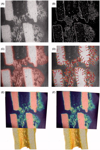
In order to apply the GHT, we first created a template from the ESEM/BSE image (Figure 3, Template creation) by computing its gradient vector field and its magnitude field. By choosing a threshold for the gradient magnitude and setting all pixels to 1 for which the gradient magnitude was above this threshold (and all remaining pixels to 0), we obtained a binary image (Figure 4B). An optional step was to create a mask using the segmentation editor of Amira (Figure 4C). In an automatic way, we placed landmarks at pixels that had a magnitude above the threshold and were contained in the manually created mask (Figure 4D). The landmarks were placed such that no other landmark could be found within a user-specified neighborhood. For each landmark, we used the gradient vector as its normal (Figure 4D, arrows). The main reason for using the additional manually created mask was that changes within the sample shape and structure occurred that were caused by embedding, drying and sectioning of the sample after µCT scanning. This sample processing resulted, for example, in cracks through the bone material. Finally, if the user was not satisfied with some of the automatically placed points, these could be interactively moved or deleted from the set. This completed the template creation.

Figure 4. Visualization of the different steps of the registration process. Panel A shows the original backscattered electron (ESEM/BSE) image. In panel B, all pixels of the ESEM/BSE image where the magnitude of the gradient is above a certain threshold are shown in white, all others in black resulting in a binary image. In panel C, the mask is depicted in red on top of the ESEM/BSE image. Creating this mask is typically a manual step. Panel D shows landmarks that were placed automatically, according to the following three rules: (i) the gradient magnitude is above a certain threshold (white pixels in binary image, panel B), (ii) they are within the mask (depicted in panel C), and (iii) no other landmark is within a user-defined neighborhood. Additionally, the image visualizes their associated gradient vectors. Panel E gives one of the n initial positions obtained by the GHT. Panel F shows the final position resulting from the initial position in panel E after the fine registration process. In panels E and F, Amira’s Colorwash tool is used to blend the slice through the µCT model with the ESEM/BSE image. Here, the gray values of the ESEM/BSE image are multiplied with the pseudocolors representing the slice through the µCT, which is shown in the back.

Preprocessing of the µCT data

Apart from creating the template, a further preprocessing step was required before the GHT could be applied (Figure 3, Gradient computation). We computed the gradient vector field of the µCT data as well as the magnitude field. From the magnitude field we created a binary mask by setting all voxels to 1 that had a gradient magnitude above a chosen threshold. This threshold was most likely different from the magnitude threshold used in the creation process of the template of the ESEM/BSE image. The selection of the threshold was visually supported by displaying the gradient magnitude with Amira’s Volren module. A compromise between too few and too many voxels had to be found. The main purpose of the binary mask was to speed up the computation of the GHT. Only voxels with a binary value of 1 were considered.

Application of generalized Hough transform

The GHT module implemented in Amira used three inputs: the template (see the section “Creation of the template from the ESEM/BSE image”), the gradient vector field of the µCT dataset, and the binary mask of the µCT dataset (see the section “Preprocessing of the µCT data”). Further parameters of the module were the rotations that were applied to the template. For registering the bone images, we rotated the template primarily around the major axis of the bone and only to a small extent (approximately ±15°) around the two minor axes. However, since we wanted to compare a 3D µCT dataset with a 2D template, we could not apply the GHT directly to the 3D gradient field of the µCT dataset. Instead, for each orientation of the template, we projected the gradient vectors of the µCT dataset into the plane of the 2D template. Using this, we were able to adapt the GHT to our needs and to appropriately register 2D images into 3D references. The subsequent steps of our registration procedure, including the GHT are sketched in Figure 3. One example of an initial position computed with the GHT is given in Figure 4(E). Hence, the GHT provided a set of initial positions with already relatively good results by analyzing mainly the contour of the bone.

Image-based optimization

Using the ESEM/BSE image as model and the µCT dataset as reference, the AffineRegistration module of Amira was used to optimize the best initial registrations obtained from the GHT. We usually used the best 10–20 initial registrations. From these, the final registrations were computed (Figure 3). This fine registration process required relatively good matches as starting positions, which were delivered as results by the GHT tool and then improved using the AffineRegistration module. We believe that the main reason for requiring good starting positions was the large number of local optima for the image-based registration problem. For all initial and all final positions, we computed metric values using mutual information. This enabled a comparison of the different positions and an observation of the improvement of registration during the fine registration process. An example of a final position is shown in Figures 4(F) and 6(D), which resulted from the initial position given in Figure 4(E). To compare the ESEM/BSE image and the slice through the µCT that was found by the registration procedure, we used Amira’s Colorwash tool (Figures 4E and F, and 6D). This module enables one to blend the two datasets by multiplying the gray values of the ESEM/BSE image with pseudocolors representing the slice through the µCT.

Figure 5. Results from nanoindentation and synchrotron small angle X-ray scattering experiments (SAXS). Panel A shows a backscattered electron image (compare Figure 1E) of a non-critical-size femoral osteotomy, six weeks post-osteotomy. The four colored boxes refer to the analyzed areas in panels B to E, which are shown in higher resolution. Panel B to D visualize nanoindentation measurement results showing the indentation modulus E _r color-coded. Panel E demonstrates small angle X-ray scattering results giving the degree of orientation (ρ parameter) and the predominant orientation (bar-coded by length and orientation) as well as the mean thickness (T parameter) of the mineral particles (color-coded).

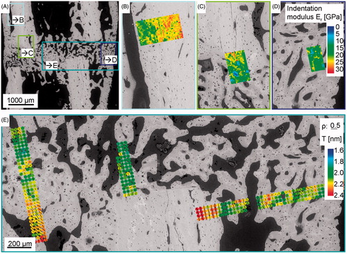
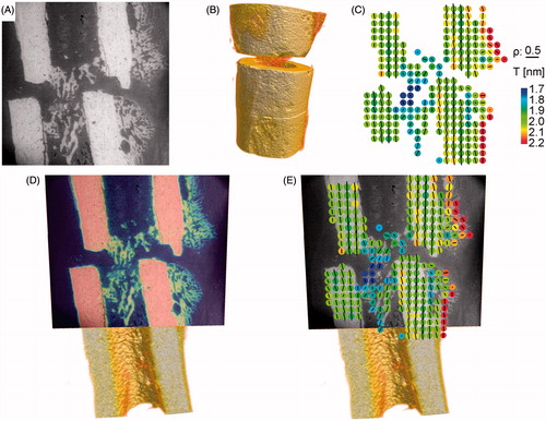
Figure 6. Illustration of registration process. Three datasets are included in the registration process; the backscattered electron image (ESEM/BSE) (panel A), the μCT as volume rendering (panel B) and the result of an experiment (here: SAXS) (panel C) of a non-critical-size rat femoral osteotomy, three weeks post-osteotomy. Panel D shows the result of the described registration process where the ESEM/BSE image is fitted into the µCT dataset. Panel E visualizes the experimental data integrated into the 3D µCT reference frame.

Scripting

Several scripts were implemented to automate parts of the workflow and to simplify the whole registration process. For example, the template creation was steered by a script. The gradient vector field computation of the µCT dataset was supported by another script. For preparing the GHT, a third script was used.

Exemplary registration and evaluation

The steps of the registration process are illustrated for one example in Figure 4. Figure 4(E) gives the result of the GHT that was used as one initial position for further refinement. Figures 4(F) and 6(D) show the resulting final position found with the refinement process. Obviously the final results (Figure 4F) further improved the outcome of the GHT (Figure 4E). A detailed visual analysis comparing the section obtained through µCT and ESEM/BSE showed that there were only very small differences. When choosing the best fit within 10–20 final positions, the quality was visually evaluated, but could also be measured quantitatively; Amira always calculated a metric value, the mutual information, to optimize the registration. This enabled us to find the best matching out of several final positions, but also to quantitatively assess the quality of the registration result and to compare the results for different samples.

Since no ground truth was available for the applications presented in the previous section, we conducted the following simple experiment to evaluate our methods. From 11 datasets we extracted two arbitrary oblique slices with main orientation along the major axis of the bone but not parallel to it. We then applied the same workflow as for the “real” application. In all cases the exact position of the extracted slice was found without any visually observable differences to the original location.

Running time

All computations were done in parallel on four CPU cores. The measured timings for the computation of the GHT varied between 10 and 25 min while the image-based optimization took less than 1 min per starting position. Since we used 10 starting positions, the overall time for the registration was less than 35 min. The creation of the mask for the GHT template is on the order of one minute and was accomplished using the segmentation editor of Amira. In summary, including the time needed for evaluating the results, a single dataset could be processed in less than one hour.

Discussion

Main achievements

The general registration process of experimental data consisted of two subsequent steps, (I) a manual registration of results from the characterizing methods into ESEM/BSE images (Figure 5), and (II) a semi-automatic registration of the ESEM/BSE images into the µCT models. With step II we obtained a transformation that could be recapitulated with the result of step I to receive the registration of experimental data into the 3D µCT references (as shown in Figure 6E). Here, we discuss the results of step II, as step I is well established and further examples can be found in a previous publication (23).

Our main achievements are (i) the development of a semi-automatic registration tool allowing quantification and comparison of registration quality. By considering the obtained metric values, one can observe whether the registration result gets better, can choose the quantitatively best registration from the obtained ones, can evaluate the quality of the registration result and compare the quality among the different samples. Using mutual information, the highest metric value indicates the best analytical result. However, we do not necessarily obtain the global optimum using this approach. To improve the change of getting close to the optimum, we employed a multi-start approach. Applying the registration tool delivers (ii) an exact 3D location of 2D experimental data enabling better interpretation of results. Furthermore, we demonstrate that (iii) ESEM/BSE images are particularly suited for semi-automatic registration. By applying the tool, we found how to (iv) optimize the sample preparation and processing in order to produce less artifacts, such as cracks or at least how to organize the order of the different steps to have the same state of the sample for all measurements.

Necessity of knowing the exact 3D location

The data illustrate the importance of knowing the exact position of 2D slices within the 3D object bone (Figure 2). An even better impression of the 3D situation is obtained by rotating and sliding into the visualized object. We therefore included a supplementary video (Video S1), which shows 3D volume renderings of the µCT results of both, the osteotomy and the whole bone, rotated around the bone’s long axis. It depicts the plane, where further experiments were performed, as it was determined with the registration routine and finally visualizes the synchrotron X-ray scattering results integrated into the 3D model. Regarding only the ESEM/BSE image of the osteotomy (Figure 2A), the sample section appeared to be well chosen and cut along the long axis and in the center of the long bone. Integrating the sample section into the reference frame revealed that our cutting plane was at the side, instead of in the center of the long bone (Figure 2D and E, locally and within the whole bone). This information was very important to correctly interpret our experimental data, especially when the analyzed properties became direction dependent. For example, properties could be anisotropic within the material, as has been shown with the hardness and indentation modulus within cortical bone (nanoindentation results, see Figure 5B–D). As previously described (29), rat long bones have a lamellar structure only at the endosteal and/or periosteal border of the cortex, called the circumferential lamellar bone. This cortical bone part has anisotropically distributed mechanical properties showing lower indentation modulus values than the central part when indented transversally (29), but higher values when indented longitudinally (23). Thus, even tilting the section could influence the result and would be important to take into account. Another example, where knowledge of specimen location is important, is in many experiments aimed at investigating structure and especially orientation within this structure. Bone consists of hydroxyapatite platelets that are embedded within a collagen matrix (4,5) and both, the platelets and the collagen fibrils are reported to be aligned along with the long axis of the bone. Small angle X-ray scattering experiments lead to parameters describing the degree of orientation (ρ parameter) and the predominant orientation of the hydroxyapatite particles (10) within the collagen matrix (see Figure 5E, visualized for every measurement point as direction of small black bar). It is possible to rotate the sample during the measurement and thereby obtaining 3D information on shape, size and arrangement of the particles (30). This is also the optimal way to correctly interpret the obtained data. However, this procedure is extremely time-consuming and only feasible with particular sample geometry. Therefore, it is necessary to at least know the orientation of the plane to appropriately interpret the SAXS results (see also supplementary text and Figure S3). Other methods, such as the Picrosirius Red staining analyzed with polarization microscopy, are used to visualize the orientation of the collagen fibers (21). Whenever investigating the orientation of the bone material, it is essential to know if the analyzed section is tilted or if it is located in the center or rather at the side of the long bone.

ESEM/BSE images as methodic link

ESEM/BSE images seem to be well suited for semi-automatic registration in µCT datasets. In contrast to most other 2D imaging techniques, such as light microscopy and histological staining techniques, backscattered electron imaging visualizes identical features and details in a similar way as those visualized in µCT data. Both techniques are based on the same physical principles, the Z-contrast, and therefore both show bone and its structure in gray values, depending on the electron density of the tissue and thus on its mineralization level. Based on these similarities, the outer shapes generated by the template formation processes and the gradients in preparation for the GHT enabled us to find an acceptable initial position that could then be refined to an excellent final position.

Stability, flexibility and limitations of the tools

We analyzed the registration process with µCT datasets in different resolutions produced by different µCT scanners, and registered data of different sample types, critical (5 mm) and non-critical (1 mm) femur osteotomy samples, after different periods of healing, three, four and six weeks post-osteotomy (see Figure 1C–E and S1). In general, in all cases we obtained satisfying results, and in most cases very good results. However, the critical-sized osteotomy samples were more difficult to handle, most probably due to the sample processing that occurred in between the two imaging processes. µCT scans were performed on native samples, and backscattered electron images were made on dehydrated, PMMA-embedded and cut samples. Obviously, the critical-sized osteotomies that failed to heal over the experimental period allowed a greater amount of interfragmentary movement compared to the smaller osteotomies. After harvesting the samples, an increased instability of the osteotomized femurs may have led to deformations, including shrinking and enlarging of the gap, but also to misalignment of the two parts. Additionally, we saw crack formation in all samples, probably accrued during dehydration. These, however, could be coped with by masking the ESEM/BSE images. Nevertheless, for both non-critical and critical healing samples, we have to state that the sample preparation process, namely the dehydration and PMMA embedding caused immense changes in the sample shape, commonly referred to as shrinkage artifact that has to be considered in future experimental designs. For further experiments, it would be preferable to perform tomography scanning after dehydration and embedding. However, in this study we used already existing datasets (µCT volumes from non-embedded samples and ESEM/BSE images from PMMA-embedded samples). Even with these non-optimal data, the registration process worked well and we could therefore describe one possible way to handle artifacts, such as cracks that complicate registration processes.

Combination of different 2D methods and 3D µCT data

Generally, combining different measurement methods and integrating their results into a 3D frame is nowadays a common task to answer specific research questions (31). Based on the fact that bone is a mineralized biological tissue, the semi-automatic registration of 2D slices into a 3D volume was realized and results were now obtained quickly, with only a minimum amount of manual labor. So far, applying automatic registration tools was only possible if relatively good matches were already obtained by hand. Registering 2D data in 3D reference models does not only help to better interpret the obtained data, but also gives possibilities for generalizations. Characterizing methods, such as nanoindentation and X-ray scattering are usually in high resolution and are very time-consuming and therefore restricted to small selected areas. By looking first at the 2D-2D registration process, and integrating these types of high-resolution data into ESEM/BSE images (mentioned in the section “Main achievements” as step I), one gets a better understanding of the results. The ESEM/BSE images are in high resolution, but also show larger structures. This approach allows one to draw assumptions in regard to bigger parts of the structure or areas having the same structure and conditions. Looking at Figure S2(A and B), we see that the orientation of the mineral particles follows the curvature of the bony closure of the marrow cavity (23). We could then suggest that the orientation, following this arc-shaped closure is not only like that in this small measured part, but also within this whole structure. On the other hand, we could expect the same orientation behavior in similarly structured closures of other samples. Furthermore, it would help to more precisely define areas for further measurement steps. To approach a 2D-3D registration of the results of this first step, we used ESEM/BSE as methodic link between the characterizing measurements and the 3D µCT models. We saved the transformation that registered the ESEM/BSE image with the µCT reference, found with the registration procedure (which is step II). We were then able to recapture this transformation with the result of step I. Hence, we could visualize and comprehend our 2D measurement results, that is, the ultrastructural, compositional and mechanical properties of the bone material, in a more complete way. By embedding them into the 3D model, we would even be able to generalize the conclusions in a 3D way, to draw further assumptions, and to understand bone as a hierarchically organized 3D structure with its many different characteristics.

In conclusion, our workflow has been tested primarily on image data obtained from bone structures, but we believe that it is general enough to be applied in other applications [see for example the work of Handschuh et al. (31)].

Supplementary material available online

Supplementary text, Figures S1, S2, S3, Video S1.

Acknowledgments

The authors would like to thank Agnes Ellinghaus, Carolin Schwarz and Mario Thiele for their support in performing the animal surgeries, sample preparation and µCT imaging. We acknowledge Miheer Shah for performing further µCT scans. We would also like to thank Chenghao Li and Stefan Siegel for helping to perform the synchrotron X-ray scattering experiments at the µspot beamline of BESSY II (Berliner Elektronenspeicherring-Gesellschaft für Synchrotronstrahlung, Helmholtz-Zentrum Berlin, Germany),and the BSRT (Berlin-Brandenburg School for Regenerative Therapies) for scientific support.

Declaration of interest

The authors report no conflicts of interest. The authors alone are responsible for the content and writing of the paper.

The authors acknowledge the DFG (Deutsche Forschungsgemeinschaft, FR 2190/4-1 Gottfried Wilhelm Leibniz-Preis 2010) and the MPG (Max-Planck-Gesellschaft) for financial support.

References

- Baron RE. Anatomy and ultrastructure of bone. In: Favus MJ, ed. Primer on the metabolic bone diseases and disorder of mineral metabolism. 3rd ed. Philadelphia, PA: Lippincott-Raven; 1996:3–10
- Shapiro F. Bone development and its relation to fracture repair. The role of mesenchymal osteoblasts and surface osteoblasts. Eur Cell Mater 2008;15:53–76
- Liu YF, Manjubala I, Schell H, Epari DR, Roschger P, Duda GN, Fratzl P. Size and habit of mineral particles in bone and mineralized callus during bone healing in sheep. J Bone Miner Res 2010;25:2029–38
- Fratzl P, Gupta HS, Paschalis EP, Roschger P. Structure and mechanical quality of the collagen-mineral nano-composite in bone. J Mater Chem 2004;14:2115–23
- Weiner S, Wagner HD. The material bone: structure mechanical function relations. Annu Rev Mater Sci 1998;28:271–98
- Fratzl P, Weinkamer R. Nature's hierarchical materials. Prog Mater Sci 2007;52:1263–334
- Kerschnitzki M, Wagermaier W, Roschger P, Seto J, Shahar R, Duda GN, Mundlos S, Fratzl P. The organization of the osteocyte network mirrors the extracellular matrix orientation in bone. J Struct Biol 2011;173:303–11
- Roschger P, Gupta HS, Berzlanovich A, Ittner G, Dempster DW, Fratzl P, Cosman F, Parisien M, Lindsay R, Nieves JW, Klaushofer K. Constant mineralization density distribution in cancellous human bone. Bone 2003;32:316–23
- Oliver WC, Pharr GM. An improved technique for determining hardness and elastic-modulus using load and displacement sensing indentation experiments. J Mater Res 1992;7:1564–83
- Rinnerthaler S, Roschger P, Jakob HF, Nader A, Klaushofer K, Fratzl P. Scanning small angle X-ray scattering analysis of human bone sections. Calcified Tissue Int 1999;64:422–9
- Hildebrand T, Laib A, Muller R, Dequeker J, Ruegsegger P. Direct three-dimensional morphometric analysis of human cancellous bone: microstructural data from spine, femur, iliac crest, and calcaneus. J Bone Miner Res 1999;14:1167–74
- Cann CE, Genant HK, Kolb FO, Ettinger B. Quantitative computed-tomography for prediction of vertebral fracture risk. Bone 1985;6:1–7
- Genant HK, Engelke K, Fuerst T, Gluer CC, Grampp S, Harris ST, Jergas M, Lang T, Lu Y, Majumdar S, Mathur A, Takada M. Noninvasive assessment of bone mineral and structure: state of the art. J Bone Miner Res 1996;11:707–30
- Zitova B, Flusser J. Image registration methods: a survey. Image Vision Comput 2003;21:977–1000
- Pluim JP, Maintz JB, Viergever MA. Mutual-information-based registration of medical images: a survey. IEEE T Med Imaging 2003;22:986–1004
- Goshtasby A. 2-D and 3-D image registration for medical, remote sensing, and industrial applications. Hoboken (NJ): A John Wiley & Sons, Inc; 2005
- Modersitzki J. Numerical methods for image registration. Oxford: Oxford University Press; 2004
- Osechinskiy S, Kruggel F. Slice-to-volume nonrigid registration of histological sections to MR images of the human brain. Anat Res Int 2010;2010:287860
- Ferrante E, Paragios N. Non-rigid 2D-3D medical image registration using Markov random fields. In: Mori K, Sakuma I, Sato Y, Barillot C, Navab N, eds. Medical image computing and computer-assisted intervention – MICCAI 2013. Berlin, Heidelberg: Springer; 2013:163–70
- Ballard DH. Generalizing the Hough transform to detect arbitrary shapes. Pattern Recogn 1981;13:111–22
- Mehta M, Schell H, Schwarz C, Peters A, Schmidt-Bleek K, Ellinghaus A, Bail HJ, Duda GN, Lienau J. A 5-mm femoral defect in female but not in male rats leads to a reproducible atrophic non-union. Arch Orthop Traum Su 2011;131:121–9
- Schwarz C, Wulsten D, Ellinghaus A, Lienau J, Willie BM, Duda GN. Mechanical load modulates the stimulatory effect of BMP2 in a rat nonunion model. Tissue Eng Part A 2013;19:247–54
- Hoerth RM, Seidt BM, Shah M, Schwarz C, Willie B, Duda GN, Fratzl P, Wagermaier W. Mechanical and structural properties of bone in non-critical and critical healing in rat. Acta Biomater 2014;10:4009–19
- Johnson R. Environmental scanning electron imaging: an introduction to ESEM®. 2nd ed. Eindhoven: Robert Johnson Associates, Philips Electron Optics; 1996
- Roschger P, Fratzl P, Eschberger J, Klaushofer K. Validation of quantitative backscattered electron imaging for the measurement of mineral density distribution in human bone biopsies. Bone 1998;23:319–26
- Manjubala I, Liu Y, Epari DR, Roschger P, Schell H, Fratzl P, Duda GN. Spatial and temporal variations of mechanical properties and mineral content of the external callus during bone healing. Bone 2009;45:185–92
- Hough PVC. Method and means for recognizing complex patterns. 1962; U.S. Patent 3069654
- Stalling D, Wetserhoff M, Hege H-C. Amira: a highly interactive system for visual data analysis. In: Delvin HC, Johnson CR, eds. The visualization handbook. Elsevier; 2005:749–67
- Shipov A, Zaslansky P, Riesemeier H, Segev G, Atkins A, Shahar R. Unremodeled endochondral bone is a major architectural component of the cortical bone of the rat (Rattus norvegicus). J Struct Biol 2013;183:132–40
- Seidel R, Gourrier A, Kerschnitzki M, Burghammer M, Fratzl P, Gupta HS, Wagermaier W. Synchrotron 3D SAXS analysis of bone nanostructure. Bioinspir Biomim Nan 2012;1:123–31
- Handschuh S, Baeumler N, Schwaha T, Ruthensteiner B. A correlative approach for combining microCT, light and transmission electron microscopy in a single 3D scenario. Front Zool 2013;10:44