Sea-ice cover anomalies in the Arctic Basin associated with atmospheric variability from multi-decadal trends to intermittent quasi-biennial oscillations

Abstract

Arctic Ocean sea ice has been diminishing since 1970, as shown by National Snow and Ice Data Center data. In addition to decadal variability, low ice anomalies in the Pacific–Siberian region have been occurring at shorter timescales. The influence of the widely-known Northern Annular Mode (NAM) occurs across all seasons. In this study, empirical orthogonal function (EOF) analysis was applied to sea-level pressure in National Centers for Environmental Prediction Reanalysis data for 1960–2007, showing the NAM to be the leading mode of variability and the Arctic Dipole Mode (ADM) to be the second leading mode. The ADM changes markedly across seasons. In autumn–winter, it has a pole over Siberia and a pole over Greenland, at opposite signs at a several-year scale, whereas the spring–summer ADM (ADMSS) has a pole over Europe and a pole over Canada. In the 1980s, the most influential mode shifted from the NAM to the ADM, when the Pacific sector had low ice cover at a 1-year lag from the positive ADM, which was marked by low pressure over Siberia. In years when the ADMSS was pronounced, it was responsible for distinct ice variability over the East Siberian–Laptev seas. The frequency separation in this study identified the contributions of the ADM and ADMSS. Effects of the latter are difficult to predict since it is intermittent and changes its sign biennially. The ADM and ADMSS should be closely watched in relation to the ongoing ice reduction in the Pacific–Siberian region.

This article repeats an error in the list of authors of an article published in the Journal of Oceanography. Please see the erratum issued by the Journal of Oceanography: http://www.terrapub.co.jp/journals/JO/abstract/2010/6606/66060885.html

• Sea ice
• sea-level pressure
• Arctic
• interannual variability
• EOF analysis

Declining over the past 40 years, the sea-ice cover in the Arctic Ocean has reached the extreme condition shown in Fig. 1, while its decadal variability has increased (e.g., Wang & Ikeda 2000). This raises the possibility that the sea-ice cover will become seasonal in the near future. Actually, the sea-ice decrease seems to be occurring more rapidly than the projection in the fourth assessment report of the Intergovernmental Panel on Climate Change (Solomon et al. 2007), in which the ice cover in summer was predicted to become minimal near the end of the 21st century (Stroeve et al. 2007). The summer ice cover hit a record low in 2007, prompting some specialists to suggest that it might disappear by 2020. Although such an early disappearance may not occur—there is significant interannual variability that must be taken into consideration—there is an urgent need to examine the mechanisms that contribute to the rapid ice decrease.

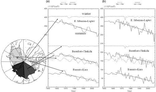
Fig. 1  Ice-cover trends and variabilities in three regions: the Beaufort–Chukchi seas, the East Siberian–Laptev seas and the Barents–Kara seas. In (a) the ice-cover time series is shown with the 3-year Hanning filter applied to the original series, shown in (b).

Recently archived data ranging from clouds and the atmospheric boundary layer to geochemical components in the Arctic Ocean have been analysed in order to gain insight into Arctic environmental change that may occur in response to global warming or as part of natural variability. The results include the following signals in the second half of the last century. The cloud cover increased and was estimated to contribute to ice reduction through the radiation balance at a magnitude similar to the ice-albedo feedback (Ikeda et al. 2003). The stratosphere was cooling in a manner consistent with global warming (Makshtas et al. unpubl. presentation). The polar vortex was a major cyclonic circulation in the Arctic atmosphere and had more significant decadal oscillations than the trend (Thompson & Wallace 1998). The geochemical data indicated that vertical motion in the ocean interior was responding to the variable polar vortex (Ikeda et al. 2005).

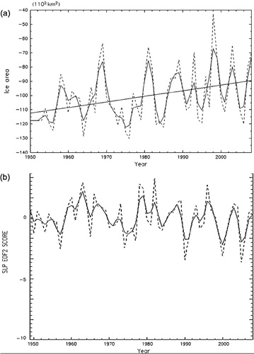
In the Arctic, the most pronounced atmospheric pattern—at least up to the turn of the century—was the Northern Annular Mode (NAM), which was first reported as the Arctic Oscillation (AO) by Thompson & Wallace (1998). Various studies have addressed whether the NAM/AO or the North Atlantic Oscillation (NAO) is dynamically more meaningful. The horizontal pattern is the intensified/weakened polar vortex, with a significant vertical coherence from the surface to the stratosphere. The decadal signal had clear peaks of the positive NAM/AO around 1973, 1982 and 1990, coinciding with strong polar vortex, as shown in Fig. 2. Mysak & Venegas (1998) claimed that the negative ice anomalies occurred around these peaks of the positive NAM/AO, propagating from the Beaufort–Chukchi seas and the East Siberian–Laptev seas to the Barents–Kara seas in several years, although the phase shift between the positive NAM/AO and the negative ice anomalies was not pinpointed. Polyakov and Johnson (2000) used a coupled ice–ocean model and reasonably simulated the ice-cover oscillations as well as ocean interior responses to the NAM/AO, but did not provide clear information on the phase shift.

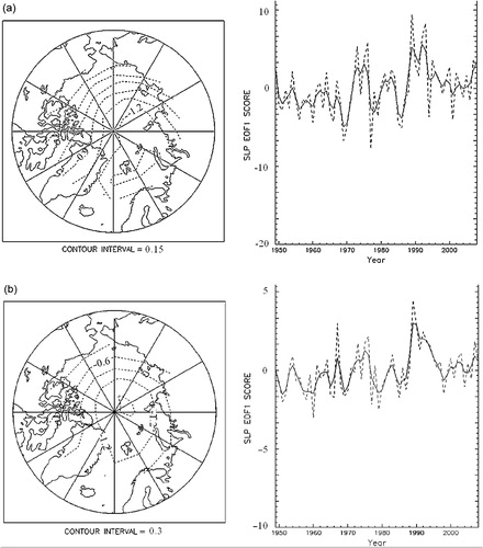
Fig. 2  The horizontal structures and time series of the first empirical orthogonal function (EOF1) for sea-level pressure (SLP) and the Northern Annular Mode/Arctic Oscillation in (a) winter (Dec.–Feb.) and (b) the average for a whole year north to 70°N. The solid lines show the time series with the 3-year Hanning filter applied on the original time series, which is indicated with dashed lines. The horizontal distributions were standardized with the average of the variance so that the time series represent standard deviations.

Inconsistent with the findings of Mysak & Vendegas (1998), a negative ice anomaly occurred around 1998 in the Beaufort–Chukchi seas but did not correlate with the NAM/AO. Post-1990, the variability cycles seem to be shorter than a decade in the Beaufort–Chukchi and Barents–Kara seas. While sea ice has been diminishing in the entire Arctic Basin, the reduction is more significant in the Pacific sector in the last 10 years (Fig. 1). An immediate question is how crucial wind-driven ice motion is for a negative ice anomaly in the Pacific sector. Once a southerly wind pushes sea ice away from the coastal region in summer, solar radiation effectively heats the ocean and accelerates ice melting. This effect was found to be a major factor contributing to the record low in sea-ice cover in the East Siberian Sea during the summer of 2007 (Kwok 2008). Ogi & Wallace (2007) attributed sea-ice reduction to air temperatures increases during the last two decades and to wind-driven ice motion. Zhang et al. (2008) proposed a rapid change in atmospheric circulation over the Arctic prior to the 2007 record, in which the new pattern included a low pressure anomaly over Siberia. Wang et al. (2009) called this pattern the Dipole Anomaly (DA) and showed a correlation with the low ice condition in the Beaufort–Chukchi seas since 1995. Ogi et al. (2008) found a multiple regression of the summer ice cover on the atmospheric pattern and the multi-year ice cover in the spring for the last 30 years, suggesting the importance of spring pre-conditioning for the ice-cover anomalies in summer and fall.

In this paper, the composite analysis of atmospheric effects reported by Wang et al. (2009) was extended to a systematic statistical analysis, along with distinguishing the variability into the frequency space from biennial to decadal scales over the period from 1950 to 2007. The Arctic atmospheric circulation was analysed to find correlations with ice anomalies in the Pacific, Siberian Shelf and Atlantic sectors of the Arctic Ocean in order to explore the cause of the ice-cover variability ranging from multi-decadal trends to biennial oscillations. These results yield insights into possible mechanisms responsible for the rapid ice decrease that has occurred in the last 10 years. Since responses of basin-scale ocean circulation take longer than sea ice, the study reported here looks for variability mechanisms by distinguishing a biennial oscillation, which is expected to represent mainly responses of ice motion and the surface mixed-layer, from longer-period oscillations. In this paper, analysis of the longer-period oscillations for the NAM/AO is presented first, followed by the ADM. Then the biennial oscillations are examined. The results are then discussed in the context of year-by-year Arctic sea-ice prediction and its projection in the 21st century.

Low-pass filtered sea-ice cover variability with NAM/AO

Sea-level pressure (SLP) fields were analysed to examine the effects of atmospheric circulation on sea-ice cover. The analyses were started with the first empirical orthogonal function (EOF). Since the focus of this study is on the effects on the ice cover in the Arctic Basin, the analysis domain was restricted to north of 70°N, as done by Overland & Wang (2010). The US National Centers for Environmental Prediction/National Center for Atmospheric Research (NCAR/NCEP) reanalysis data were used under consideration of the area represented by each data point, where the points were chosen in proportion to the size of the latitudinal circles from the points regularly distributed in the longitude–latitude grids. The first EOFs were obtained from the monthly mean data separately for four seasons: winter (Dec.–Feb.), spring (Mar.–May), summer (Jun.–Aug.) and autumn (Sep.–Nov.). They have horizontal patterns consistent among all the four seasons, although only the winter one is shown in Fig. 2a. This mode—the NAM/AO—essentially contains fluctuations between stronger and weaker phases of the polar vortex. The atmospheric circulation near sea level is represented by weaker and stronger phases of the Beaufort High over the Canada Basin, corresponding to the stronger and weaker phases of the polar vortex, and defined as the positive and negative NAM/AO, respectively.

Although a trend is usually removed from the original time series prior to principal component analysis, this was not done in the present study, following Thompson & Wallace (1998). The trends are minor, and removing them made no fundamental change in the horizontal patterns. In addition, the horizontal distributions were standardized with the average of the variance so that the time series represent standard deviations.

The whole year sea-level pressure was analysed to show the first EOF (Fig. 2b). The horizontal structures are similar between the winter and annual modes. The winter time series well represents the annual one: the two time series have a correlation coefficient of 0.86. As shown in Table 1, the standard deviation of the annual component is less than half of the winter one and is smaller than any seasonal components. This result is reasonable, since an average over a longer time span partially cancels anomalies in individual seasons. In spite of the smaller annual component, its effects over time are not necessarily smaller because it works for a longer time.

Table 1 Standard deviations of the total sea-level pressure variabilities and their first and second empirical orthogonal functions (EOFs) in four seasons—winter (Dec.–Feb.), spring (Mar.–May), summer (Jun.–Aug.) and autumn (Sep.–Nov.)—along with spring–summer (Mar.–Aug.) and the entire year. The values are spatial averages of sea-level pressure deviations (hPa): each EOF has a time series with the standard deviation shown in the table, and a spatial pattern with the average variance of unity. The analysis was carried out for the period 1950–2008. The first and second EOFs occupy about 60% and 15% of the total variance, respectively, while the amplitudes of the second EOFs are about half of the first EOFs.

	Winter	Spring	Summer	Autumn	Spring and summer	Entire year
Total	4.27	3.16	2.24	2.81	1.99	1.82
1st EOF	3.41	2.47	1.64	1.96	1.51	1.44
2nd EOF	1.50	1.17	0.84	1.14	0.76	0.65

Quasi-biennial fluctuations are visible in the NAM/AO, while general circulation in a coupled ice–ocean system is expected to respond to longer-period oscillations. Hence, the 3-year Hanning filter was applied to separate the biennial component from the longer-period one, by replacing p(i) with 0.25 p(i − 1) + 0.5 p(i) + 0.25 p(i + 1), where i is an index for the year in question. The resultant component was a low-pass filtered one, while the difference between the original and low-pass filtered components was defined as a high-pass filtered component. The standard deviations of the low-pass and high-pass filtered NAM/AO are listed in Table 2. The low-pass filtered component is a little larger than the high-pass filtered one. Note that the time series were de-trended and analysed for the period after 1960, when the sea-ice cover data are more reliable than before 1960. Below, the low-pass filtered components are discussed first, followed by the high-pass filtered components.

Table 2 Standard deviations of the low-pass filtered and high-pass filtered Northern Annular Mode (NAM)/Arctic Oscillation (AO), Arctic Dipole Mode (ADM) and the spring–summer ADM (ADMSS), as well as the summer ice-covered areas in the three regions. The three regions are the Beaufort–Chukchi seas (BC), the East Siberian–Laptev seas (EL) and the Barents–Kara seas (BK). The original time series were de-trended and smoothed by the 3-year Hanning filter to produce the low-pass filtered time series. The differences between the de-trended original and smoothed data are defined as the high-pass filtered ones. The units are hPa for the spatial means of sea-level pressure deviations and 110² km² for the ice covers. The analysis was carried out for the period 1960–2008.

	NAM/AO	ADM	ADMSS	BC	EL	BK
Low-pass	2.20	0.95	0.42	7.6	10.1	8.7
High-pass	2.03	0.83	0.55	6.6	9.5	6.5

The low-pass filtered NAM/AO shows very clear decadal oscillations from 1965 to 1995 but minor variations after this period (Fig. 2), as previously reported by many authors. The sea-ice areas were taken from ice concentration data in the same way as in previous studies (e.g., Ikeda et al. 2003; Wang et al. 2009). The low-pass filtered ice areas also display decadal oscillations during 1965–1995, superimposed upon the declining trends (Fig. 1). The effects of the first EOF have been examined extensively (e.g., Wang & Ikeda 2000; Rigor et al. 2002) but were revisited in this study. The ice cover was reported to reduce sequentially in the Beaufort–Chukchi seas, the East Siberian–Laptev seas and the Barents–Kara seas in response to the positive phases of the NAM/AO (Mysak & Venegas 1998). In the study reported in this paper, this sequence was examined statistically.

As shown in Figs. 1 and 2, the minima in the East Siberian–Laptev seas match with the positive phases. The low-pass time series are correlated at a 90% confidence level between the winter NAM/AO and the summer ice cover, but not at a 95% confidence level (Table 3a). The minima occurred in the East Siberian–Laptev seas and, 2 years later, in the Barents–Kara seas. In the Beaufort–Chukchi seas, the ice cover increased 2 years after the NAM/AO peaks. The opposite variations between the Beaufort–Chukchi seas and the Barents–Kara seas are reasonable from the pattern of the NAM/AO, which weakens the Beaufort Gyre during the positive phase and reduces a clockwise circulation. Once the NAM/AO has a decadal oscillation, the sea-ice cover anomaly may behave as a perturbation propagating from the Beaufort–Chukchi seas to the Barents–Kara seas in 4–5 years. The statistical analysis supports this interpretation rather than a consistent anomaly propagating from the Beaufort–Chukchi seas to the Barents–Kara seas. There was a negative, but not significant, correlation between the NAM/AO and the sea ice in the Beaufort–Chukchi seas, with an advance (negative lag) of 2–3 years. No significant difference was observed between the entire period and the period dominated by the NAM/AO before 1990.

Table 3 (a) Correlations between the atmospheric variability and summer ice-cover variability for the low-pass filtered data, defined in Table 2, in relation to the Northern Annular Mode (NAM)/Arctic Oscillation (AO) and the Arctic Dipole Mode (ADM). The spring–summer ADM (ADMSS) is excluded, since it is minor. The three regions are the Beaufort–Chukchi seas (BC), the East Siberian–Laptev seas (EL) and the Barents–Kara seas (BK). (b) Correlations between the atmospheric variability and summer ice-cover variability for the high-pass filtered data, defined in Table 2. The correlation coefficients are shown for simultaneous cases (0-year lag) as well as the highest correlations among the lagged cases between 3 and −1-year lags, if they are higher than the simultaneous ones. Here, the lags in parentheses represent the years by which the ice cover lags from the atmosphere. Values in boldface indicate significant correlations at the 95% confidence level, where the numbers of degrees of freedom were calculated from the analysis periods divided by the zero auto-correlation timescales to be 20 for (a) and 30 for (b) during the analysis period 1960–2007. Note that the annual NAM/AO correlates very highly with the winter one at a correlation coefficient of 0.86.

	BC	EL	BK
(a) Low-pass filtered
NAM/AO 1960–2007	0.04/0.36(2)	−0.29	−0.20/ − 0.26(2)
NAM/AO 1960–1992	0.03/0.47(2)	−0.34	−0.22/ − 0.24(3)
ADM 1960–2007	−0.37/ − 0.41(1)	0.18	0.14
ADM 1976–2007	−0.35/−0.46(1)	0.37	0.27
(b) High-pass filtered
NAM/AO 1960–2007	−0.03/0.19(2)	−0.18/0.31(−1)	−0.04/ − 0.06(−1)
ADM 1960–2007	−0.02/−0.34(2)	0.31	0.22
ADMSS 1960–2007	−0.46/0.50(−1)	−0.84	−0.37/0.60(1)

Rigor et al. (2002) suggested that observed ice velocity fields vary in response to the NAM/AO: the ice stream in the Transpolar Drift Stream shifts toward Canadian and Eurasian sides in the positive and negative phases, respectively. In a coupled ice–ocean model, Polyakov & Johnson (2000) showed that the ocean circulation in the Arctic Basin swings between these two states. This mode mostly explains the ice reduction in the early 1970s, early 1980s and around 1990 in the Barents–Kara seas.

Low-pass filtered sea-ice cover variability with Arctic Dipole Mode

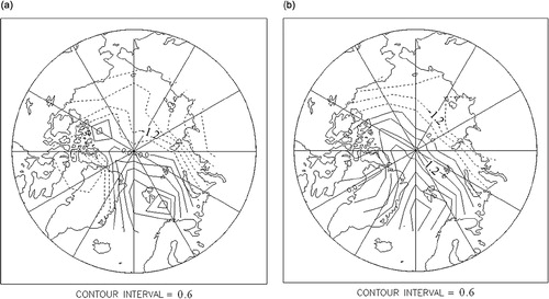
Analyses were extended to the second EOF, as done by Wu et al. (2006), whose careful analysis of the atmospheric data and ice motion data confirmed this mode as an important component for sea-ice motion in the Arctic Basin. The second EOF has been considered as a meaningful mode by Wu et al. (2006) and others, using the statistical criteria suggested by North et al. (1982). As the second EOF, the horizontal features have two poles in all four seasons. The winter one (Fig. 3a) has a positive pole located over Greenland and a negative pole over Siberia. This mode is called the Arctic Dipole Mode (ADM) in the present work. The autumn mode has a horizontal pattern similar to the winter one (figure not shown), while the autumn deviation is about two-thirds that of the winter (Table 1). The spring and summer patterns rotate clockwise by about 60°. The mode combined in spring and summer (Mar.–Aug.; Fig. 3b) is called the ADMSS. The seasonal ADM and ADMSS have pressure deviations nearly half of the NAM/AO (Table 1), whereas in the horizontal patterns the ADM and ADMSS pressure gradients are much larger than the NAM/AO (Figs. 2, 3). Since winds are related to gradients of pressure fields, which are products of the time series and horizontal patterns of EOFs, the ADM and ADMSS are expected to give forcing effects comparable to the NAM/AO.

Fig. 3  The horizontal structures and time series of the second empirical orthogonal function (EOF2) for sea-level pressure (SLP): (a) the Arctic Dipole Mode/Dipole Anomaly in winter; and (b) the spring–summer Arctic Dipole Mode (Mar.–Aug.).

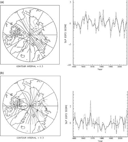
A major difference is seen in more distinct quasi-biennial components of the ADMSS (Fig. 3, Table 2). The low-pass filtered amplitude of this mode is much smaller than the winter one. The autumn mode also has a minor low-pass filtered component (figure not shown). Therefore, the rest of this section focuses on the winter ADM for the analysis of the low-pass filtered data. In the following section, the ADMSS is examined to reveal the relationship with the sea-ice cover in the same year using the high-pass filtered data.

Wang et al. (2009) studied the causes of low ice anomalies in the Canada Basin during the past 50 years by using composite analyses and examining the immediate relationship between ice cover and atmospheric variability. They showed that the low summer ice anomalies are attributable to the winter–spring dipole anomaly (DA) and also the summer DA in the same year. In the present study both of the DAs essentially correspond to the ADM and ADMSS. In the last 15 years, six occasions of low ice cover were observed in the Arctic Basin, and four of them were related to both winter–spring and summer DAs. In the present study, the high-pass and low-pass filtered components were separated. The role of ocean general circulation was also considered: a smoothed time series is more appropriate for the statistical analysis of slow oceanic responses, if there are any.

As shown in Fig. 3a, the low-pass filtered time series exhibits fluctuations at a several-year cycle after 1970. In addition to the fluctuations, there is a weak negative trend. It is noted that the positive phases had smaller amplitudes after 1990 than before 1990. By adding the mean SLP, the composite of the positive ADM in 1978, 1979, 1982 and 1996 was produced in Fig. 4, as well as that of the negative ADM in 1990, 2000 and 2005. Since the mean was added, the patterns are not anti-symmetric between the positive and negative phases. During the positive phase, the Pacific sector experienced southerly winds and sea ice was pushed seaward. The opposite tendency appeared in the negative phase. In the Atlantic sector, sea ice received weak wind stress in the positive phase, whereas sea ice was strongly pushed away from European coast of the Barents–Kara seas in the negative phase.

Fig. 4  (a) The sea-level pressure composite of the positive winter Arctic Dipole Mode in 1978, 1979, 1982 and 1996 and (b) the negative winter Arctic Dipole Mode in 1990, 2000 and 2005.

The time series were first visually examined to identify correlations between sea-ice conditions and atmospheric modes. The ice-cover areas examined were the Beaufort–Chukchi seas and the Barents–Kara seas; the difference between them was determined by subtracting values for the Beaufort–Chukchi seas from values for the Barents–Kara seas. The seasons were winter (Dec.–Feb.) and summer (Jun.–Aug.). Occurring at several-year cycles, the variability was superimposed on the positive trend. Note that since the Beaufort–Chukchi seas are almost completely covered by sea ice in winter (Fig. 1), the winter difference is similar to the ice-cover anomaly in the Barents–Kara seas. Here, only the difference is shown for summer in Fig. 5. The ADM seems to be correlated with the ice cover, which lags by a couple of years from the ADM (Table 3a). Since the ADM has strong quasi-biennial components, correlation coefficients are not consistently high between the original time series, even with 1- or 2-year lags.

Fig. 5  (a) Summer (Jun.–Aug.) sea-ice anomalies shown as the differences between the Beaufort–Chukchi seas and the Barents–Kara seas (the latter minus the former); (b) the second empirical orthogonal function (EOF2) of the sea-level pressure (SLP) in relation to the Arctic Dipole Mode. The solid lines show the time series with the 3-year Hanning filter applied on the original time series, which is indicated with dashed lines.

Table 4 shows the correlation coefficients between the winter ADM and the ice-cover difference between the Beaufort–Chukchi seas and the Barents–Kara seas in summer. Both of the time series were low-pass filtered: the Hanning filter was applied, and the trends were removed. The correlation coefficients were calculated with the ice cover, lagging by −1 to 3 years relative to the ADM. Positive correlations are found to be significant for the entire 48-year period between the ADM and the ice-cover difference with 0 and 1-year lags: the ice cover decreased (increased) over the Beaufort–Chukchi seas (Barents–Kara seas) in summers of the same year and 1 year after the positive winter ADM. In the period from 1976, the correlation is significant at a 1-year lag, while it is not at 0-year lag. This contrast implies a significant time lag, although the effects of the Hanning filter must be taken into consideration.

Table 4 Correlation coefficients between the winter Arctic Dipole Mode (ADM) and the summer ice cover of the Barents–Kara seas minus the Beaufort–Chukchi seas. All time series have been low-pass filtered. The period 1976–2007 was selected because the ADM shows great variability. The year values denote the lags by which the ice cover lags the ADM. Values in boldface indicate significant correlations at the 95% confidence level, where the numbers of degrees of freedom are 20 in 1960–2007 and 15 in 1976–2007.

Period	−1 year	0 year	1 year	2 year	3 year
1960–2007	−0.02	0.38	0.48	0.28	0.07
1976–2007	−0.08	0.38	0.48	0.19	0.09

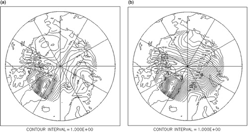
The relationship between the atmospheric pattern and the sea-ice cover was further examined using patterns regressed on the indices; similar to what is often carried out in analyses of atmospheric patterns regressed on climate indices. Since sea ice is driven by wind stresses, how sea ice is influenced by the atmosphere in seasons other than winter is a reasonable concern. With this concern in a mind, the SLP in a whole year was regressed on the summer sea-ice anomalies (Barents–Kara minus Beaufort–Chukchi seas) by taking a sum of products of SLP at each grid with the ice anomalies. The ice anomalies were lagged by 0, 1 and 2 years from the atmosphere. Here, a whole year starts in December of the previous year until November of the year in question, e.g., year 2005 refers to the period from December 2004 to November 2005. Figure 6 shows the regressed patterns with 0- and 1-year lags for the period of 1976–2006, when the ADM had clear several-year cycles. The feature considered to be most influential for the ice anomaly is an SLP gradient over the Transpolar Drift Stream. An additional important feature for the ice anomaly is a clockwise circulation in the Canada Basin. These are much more distinct with a 1-year lag, and possess characteristics similar to the winter ADM (Fig. 3a) and ADMSS (Fig. 3b), respectively.

Fig. 6  The sea-level pressure average for a whole year regressed on the summer sea ice anomalies (Barents–Kara seas minus Beaufort–Chukchi seas) with (a) zero-year and (b) one-year lags from the sea level pressure to sea ice. Here, a whole year starts in December of the previous year until November of the year in question. The ice anomalies have been normalized by their own standard deviations.

High-pass filtered sea-ice cover variability

A main objective in this section is to explore a relationship between the sea-ice cover and the atmospheric patterns at a quasi-biennial scale. First of all, how the 3-year Hanning filter separates the time series in a frequency domain was examined. In Table 5, the auto-correlations are shown for the NAM/AO, ADM and ADMSS. The original time series have no sign of statistically significant timescales. Among the low-pass filtered series, the NAM/AO possesses a statistically significant 10-year oscillation with a negative correlation at a 5-year lag, while the ADM shows only insignificant 6-year cycles. The ADMSS has no sign of oscillations. The high-pass filtered series exhibit biennial oscillations only for the ADMSS with a negative correlation at a 1-year lag and positive correlation at a 2-year lag, while the NAM/AO has 3-year cycles. Thus, the ADMSS is distinct among those atmospheric patterns.

Table 5 Auto-correlation coefficients of the Northern Annular Mode (NAM)/Arctic Oscillation (AO), the Arctic Diple Mode (ADM) and the spring–summer ADM (ADMSS), where the year values denote the time differences between the time series itself and the shifted one. The original time series were already de-trended, and the analyses were carried out for the period 1960–2007. The auto-correlation coefficient is always unity at 0 lag. Values in boldface indicate significant correlations at the 95% confidence level, where the numbers of degrees of freedom are 20 for the original and low-pass filtered data and 30 for the high-pass filtered data.

	1 year	2 year	3 year	4 year	5 year
NAM/AO
Original	0.06	−0.01	0.11	0.22	0.15
Low-pass	0.70	0.21	−0.05	−0.26	−0.38
High-pass	−0.63	0.02	0.27	−0.24	0.10
ADM
Original	0.10	−0.30	−0.10	−0.01	−0.04
Low-pass	0.55	−0.14	−0.30	−0.15	−0.02
High-pass	−0.48	−0.18	0.17	0.04	−0.09
ADMSS
Original	−0.18	0.10	0.09	−0.10	0.07
Low-pass	0.72	0.25	0.08	0.04	0.21
High-pass	−0.73	0.26	0.02	−0.10	0.06

Quasi-biennial oscillations in the sea-ice cover are energetic in the three regions, while the high-pass filtered component is dominant over the low-pass filtered component only in the ADMSS (Fig. 1, Table 2). The quasi-biennial components are shown in Fig. 7. The envelopes of the quasi-biennial oscillations have consistent time sequences between the ADMSS and the sea-ice cover in the East Siberian–Laptev seas with larger oscillations in the 1960s–70s, early 1990s and very recent years. The other consistent pair shows up as the NAM/AO and the Beaufort–Chukchi seas in the late 1970s and the mid-1990s. These possible synchronizing pairs are examined statistically later in this section.

Fig. 7  (a) High-pass filtered components of the atmospheric components, the Northern Annular Mode/Arctic Oscillation as the first empirical orthogonal function (EOF1), the Arctic Dipole Mode and the spring–summer Arctic Dipole Mode (Mar.–Aug.) as the second empirical orthogonal function (EOF2). (b) The summer (Jun.–Aug.) sea-ice anomalies in the three regions: the Beaufort–Chukchi seas, the East Siberian–Laptev seas and the Barents–Kara seas. The high-pass filtered components were produced by subtracting the 3-year Hanning-filtered data from the original data. Only the Northern Annular Mode/Arctic Oscillation is plotted by halving the amplitude.

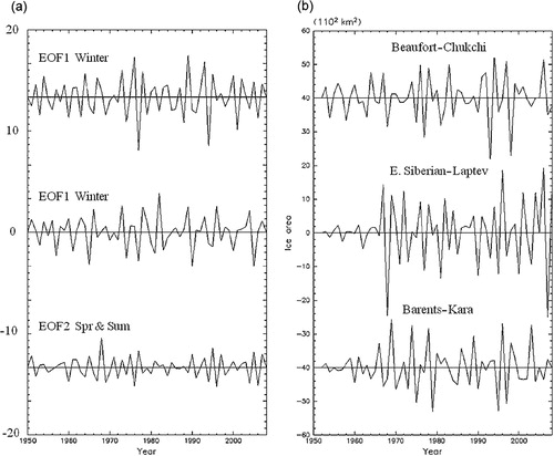
A signature in the ADMSS makes sea ice oscillate seaward and shoreward in the East Siberian–Laptev seas (Fig. 3b). The anomaly may influence the Barents–Kara seas by driving sea ice through the Transpolar Drift Stream. The NAM/AO has potential to influence the sea-ice cover by weakening or strengthening the Beaufort High so that sea-ice transport from the Beaufort–Chukchi seas may reduce or increase.

Table 3b presents the correlations between the atmospheric components and the ice-cover anomalies. The correlation coefficient is extremely high between the ADMSS and the ice cover: the positive ADMSS is simultaneously correlated with low sea-ice cover in the East Siberian–Laptev seas along with, to a lesser extent, the Beaufort–Chukchi seas. The correlation with the Barents–Kara seas is positive and higher at a 1-year lag, while it is negative and lower at a 0-year lag. The correlations are significant at a 95% confidence level, where the numbers of degrees of freedom are 30. This relationship suggests that, under the positive ADMSS, sea ice was pushed away from the East Siberian–Laptev seas and appeared as accumulation towards the Barents–Kara seas 1 year later.

Responses of sea-ice cover are shown to appear in the same year as the quasi-biennial atmospheric components much more clearly with the ADMSS than the NAM/AO and ADM. The summer ice cover in the East Siberian–Laptev seas was compared with the ADMSS and NAM/AO for individual years. The negative ice anomalies shown in Fig. 7 appeared in 1968, 1971, 1973, 1977, 1981, 1985, 1990, 1993, 1995, 1997, 2000, 2003, 2005 and 2007. These anomalies matched with the positive ADMSS in most cases, while they coexisted with the positive NAM/AO only in 1973, 1981, 1993, 1995, 2000, 2005 and 2007. In addition to the higher correlation coefficient, the comparison for each event also confirmed the role of the ADMSS on the quasi-biennial ice-cover oscillations in the East Siberian–Laptev seas. The record low in 2007 stands out, while the ADMSS does not stand out for 2007 within the time series. As discussed in work by Kwok (2008) and Wang et al. (2009), among others, seaward winds carried warm air from Siberia in summer and played dynamic and thermodynamic roles.

Summary and discussion

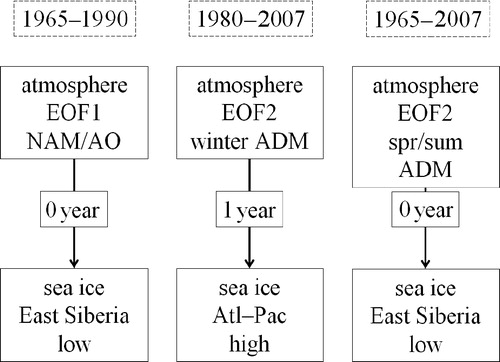
As shown in Fig. 8, which summarizes the results of this study, sea-level pressure fields were dominated by the winter pressure fields, with the NAM/AO as the first EOF and the ADM as the second EOF. The low-pass filtered sea-ice cover variability was explained by these two modes sequentially: the NAM/AO was dominant and responsible for the decadal ice-cover variability until 1990. The work reported here specifies for the first time the time lags from the NAM/AO to sea-ice anomalies in the East Siberian–Laptev seas, the Beaufort–Chukchi seas and the Barents–Kara seas by taking into consideration shifts of the Transpolar Drift Stream as a key mechanism. The most influential atmospheric mode shifted to the ADM during the 1980s, while the amplitude of the NAM/AO was reduced after 1980. The positive (negative) ADM with a low (high) anomaly over Siberia and a high (low) anomaly over Greenland induced low (high) ice cover in the Pacific sector in the summer a half-year later as well as in the summer of the next year. The ADMSS was active intermittently at a quasi-biennial scale both before and after 1980.

Fig. 8  Summary of relationships among the atmospheric modes and sea-ice cover. Transition in the most influential atmospheric mode is suggested from Northern Annular Mode (NAM)/Arctic Oscillation (AO) as the first empirical orthogonal function (EOF1) to Arctic Dipole Mode (ADM) as the second empirical orthogonal function (EOF2) during the 1980s, while the ADM in spring–summer (ADMSS) as EOF2 was significant for the entire period with some temporal non-homogeneity. The sea-ice features are specified to be low ice cover over the East Siberian–Laptev seas and the ice-cover difference (Atlantic sector minus Pacific sector) for the earlier and later periods, respectively. The time lags are presented for the lags from the atmospheric modes, positive NAM/AO, ADM and ADMSS, to the ice-cover anomalies.

The quasi-biennial variability was retrieved by subtracting the time series smoothed with the 3-year Hanning filter from the original time series. This high-pass filtered variability in sea-ice cover was distinct in summer over the East Siberian–Laptev seas and was explained by the ADMSS, i.e., the spring–summer ADM (Fig. 7). The record low ice cover in 2007 summer was attributed to the very intense ADMSS, as suggested by Kwok (2008), while another anomaly of the winter ADM came into play to reduce the ice cover in the Pacific sector for 2007–08 (Fig. 5). This finding is consistent with the suggestion by Wang et al. (2009), who explained the low ice record in the Arctic Basin by both summer and winter ADM.

Let us look at how these findings offer possibilities for sea-ice prediction in the individual regions under consideration. The quasi-biennial ADMSS occurred intermittently, making a 2-year prediction of sea-ice cover extremely difficult for the East Siberian–Laptev seas. For the Barents–Kara seas, the anomaly induced by the ADMSS may appear in the following year at an opposite sign. In the Beaufort–Chukchi seas, an interannual anomaly is attributable to the ADM at several-year scales and may continue to the following year.

The trend shows that the positive ADM weakens over the long term, with the result that the recent ADM is relatively minor. In contrast, the ADMSS has shown an increasing trend for 20 years. If the past statistics hold, these atmospheric patterns would minimize each other and have a minor impact on a decreasing sea-ice trend. In the other words, the anomalous condition of the last few years is not a direct indication that ice cover on the Arctic Ocean will soon be absent during summers.

After the record low of summer ice cover in 2007, the ice cover recovered slightly in 2008. As is well recognized, interannual variability is often more noticeable than a centennial change. Therefore, we should avoid both of the following claims: the record low in 2007 represents a rapid reduction of summer sea-ice cover as a result of global warming; and the recovery in 2008 is evidence that global warming is not occurring.

What is causing ice cover to decrease more rapidly in the Pacific sector and the Siberian Shelf remains an open question. Solar radiation and air temperature, which occur in association with the ADMSS, may be having an effect. Aagaard & Carmack (1989) reported that Pacific Water is an important source of fresh water in the Arctic Ocean. Pacific Water is also a heat source. Shimada et al. (2006) pointed out the importance of Pacific Water inflow in summer for ice reduction and suggested that this inflow works as a trigger for a more influential mechanism of ice reduction through air–sea interactions. A preliminary analysis was performed on sea level in the Bering Sea and compared with the current meter data through the Bering Strait (Ikeda 2009). The inflow of Pacific Water increased in the 1990s (Woodgate et al. 2008) and may be contributing toward the reduction of ice in the Pacific sector. Wind-driven ocean currents have also been suggested as mechanisms of the inflow variability (Mizobata et al. 2010).

In the present study, a basic concept is that the atmosphere is responsible for sea-ice cover anomalies. Overland & Wang (2010) have suggested that the ice–ocean system can be a driver of the atmosphere, e.g., a low ice-cover anomaly in summer tends to warm up the atmosphere in autumn. A robust consequence may be constrained to baroclinic structures represented by air temperature and boundary layer thickness. However, the sea-level pressure field did not show—at a time lag—a strong correlation with the ice-cover anomalies (Tables 3 and 4). It is anticipated that the ice anomalies will grow in this century; hence this feedback process might become crucial and dominant.

Acknowledgements

Financial support from the Japanese Ministry of Education, Culture, Sport, Science and Technology was fundamental to this work. Fruitful discussions with Drs J. Overland, S. Prinsenberg, J. Wang, G. Panteleev, J. Zhang, K. Mizobata and X. Zhang are much appreciated. A. Yamada is thanked for solid analyses of various data sets.

References

- Aagaard K. Carmack E.C. The role of sea ice and other fresh water in the Arctic circulation. Journal of Geophysical Research—Oceans. 1989; 94: 14485–14498. 10.3402/polar.v31i0.18690.
- Ikeda M. Mechanisms of the recent sea ice decay in the Arctic Ocean related to the Pacific-to-Atlantic pathway. Influence of climate change on the changing Arctic and sub-Arctic conditions. Nihoul J.C.J. Kostianoy A.G. Springer. Liege, 2009; 161–169.
- Ikeda M, Colony R, Yamaguchi H. & Ikeda T. 2005. Decadal variability in the Arctic Ocean shown in hydrochemical data. Geophysical Research Letters. 32, L21605., doi: 10.3402/polar.v31i0.18690.
- Ikeda M. Wang J. Makshtas A. Importance of clouds to the decaying trend in the Arctic ice cover. Journal of the Meteorological Society of Japan. 2003; 81: 179–189. 10.3402/polar.v31i0.18690.
- Kwok R. 2008. Summer sea ice motion from the 18 GHz channel of AMSR-E and the exchange of sea ice between the Pacific and Atlantic sectors. Geophysical Research Letters. 35, L03504., doi: 10.3402/polar.v31i0.18690.
- Mizobata K. Shimada K. Woodgate R. Saitoh S. Wang J. Estimation of heat flux through the Eastern Bering Strait. Journal of Oceanography. 2010; 66: 405–424. 10.3402/polar.v31i0.18690.
- Mysak L.A. Venegas S.A. Decadal climate oscillations in the Arctic: a new feedback loop for atmosphere–ice–ocean interactions. Geophysical Research Letters. 1998; 25: 3607–3610. 10.3402/polar.v31i0.18690.
- North G.R. Bell T.L. Cahalan R.F. Moeng F.J. Sampling errors in the estimation of EOFs. Monthly Weather Review. 1982; 110: 699–706. 10.3402/polar.v31i0.18690.
- Ogi M, Rigor I.G, McPhee M.G. & Wallace J.M. 2008. Summer retreat of Arctic sea ice: role of summer winds. Geophysical Research Letters. 35, L24701., doi: 10.3402/polar.v31i0.18690.
- Ogi M. & Wallace J.M. 2007. Summer minimum Arctic sea ice extent and the associated summer atmospheric circulation. Geophysical Research Letters. 34, L12705., doi: 10.3402/polar.v31i0.18690.
- Overland J.E. & Wang M. 2010. Large-scale atmospheric circulation changes are associated with the recent loss of Arctic sea ice. Tellus Series A. 62, doi: 10.3402/polar.v31i0.18690.
- Polyakov I.V. Johnson M.A. Arctic decadal and interdecadal variability. Geophysical Research Letters. 2000; 27: 4097–4100. 10.3402/polar.v31i0.18690.
- Rigor I.G. Wallace J.M. Colony R. Response of sea ice to Arctic Oscillation. Journal of Climate. 2002; 15: 2648–2663. 10.3402/polar.v31i0.18690.
- Shimada K, Kamoshida T, Itoh M, Nishino S, Carmack E, McLaughlin F, Zimmermann S. & Proshutinsky A. 2006. Pacific Ocean inflow: influence on catastrophic reduction of sea ice cover in the Arctic Ocean. Geophysical Research Letters. 33, L08605., doi: 10.3402/polar.v31i0.18690.
- Solomon S., Qin D., Manning M., Chen Z., Marquis M., Averyt K.B., Tignor M. & Miller H.L. Jr. 2007. Climate change 2007. The physical science basis: contribution of Working Group I to the fourth assessment report of the Intergovernmental Panel on Climate Change. Cambridge: Cambridge University Press.
- Stroeve J, Holland M.M, Meier W, Scambos T. & Serreze M. 2007. Arctic sea ice decline: faster than forecast. Geophysical Research Letters. 34, L09501., doi: 10.3402/polar.v31i0.18690.
- Thompson D.W.J. Wallace J.M. The Arctic Oscillation signature in the wintertime geopotential height and temperature fields. Geophysical Research Letters. 1998; 25: 1297–1300. 10.3402/polar.v31i0.18690.
- Wang J. Ikeda M. Arctic Oscillation and Arctic sea ice oscillation. Geophysical Research Letters. 2000; 27: 1287–1290. 10.3402/polar.v31i0.18690.
- Wang J, Zhang J, Watanabe E, Ikeda M, Mizobata K, Walsh J.E, Bai X. & Wu B. 2009. Is the Dipole Anomaly a major driver to record lows in Arctic summer sea ice extent?. Geophysical Research Letters. 36, L05706., doi: 10.3402/polar.v31i0.18690.
- Woodgate R.A, Aagaard K. & Weingartner T.J. 2006. Interannual changes in the Bering Strait fluxes of volume, heat and freshwater between 1991 and 2004. Geophysical Research Letters. 33, L15609., doi: 10.3402/polar.v31i0.18690.
- Wu B. Wang J. Walsh J.E. Dipole anomaly in the winter Arctic atmosphere and its association with sea ice motion. Journal of Climate. 2006; 19: 210–225. 10.3402/polar.v31i0.18690.
- Zhang X, Sorteberg A, Zhang J, Gerdes R. & Comiso J.C. 2008. Recent radical shifts of atmospheric circulations and rapid changes in Arctic climate system. Geophysical Research Letters. 35, L22701., doi: 10.3402/polar.v31i0.18690.