Interactions between topographically and thermally forced stationary waves: implications for ice-sheet evolution

ABSTRACT

This study examines mutual interactions between stationary waves and ice sheets using a dry atmospheric primitive-equation model coupled to a three-dimensional thermomechanical ice-sheet model. The emphasis is on how non-linear interactions between thermal and topographical forcing of the stationary waves influence the ice-sheet evolution by changing the ablation. Simulations are conducted in which a small ice cap, on an idealised Northern Hemisphere continent, evolves to an equilibrium continental-scale ice sheet. In the absence of stationary waves, the equilibrium ice sheet arrives at symmetric shape with a zonal equatorward margin. In isolation, the topographically induced stationary waves have essentially no impact on the equilibrium features of the ice sheet. The reason is that the temperature anomalies are located far from the equatorward ice margin. When forcing due to thermal cooling is added to the topographical forcing, thermally induced perturbation winds amplify the topographically induced stationary-wave response, which that serves to increase both the equatorward extent and the volume of the ice sheet. Roughly, a 10% increase in the ice volume is reported here. Hence, the present study suggests that the topographically induced stationary-wave response can be substantially enhanced by the high albedo of ice sheets.

• stationary waves
• ice sheets
• topographical forcing
• thermal forcing

1. Introduction

At the Last Glacial Maximum (LGM; about 20kyr ago), the Northern Hemisphere ice sheets reached their maximum extents during the last glacial-interglacial cycle. At this time, essentially the whole Canada and Northern Europe were ice covered, whereas other boreal land areas, such as Eastern Siberia and Alaska, remained ice-free (Clark and Mix, 2002; Dyke, 2004). Although the geographical extents of the LGM ice sheets are well constrained, it is still uncertain how the ice sheets arrived at the observed extents (Dyke et al., 2002; Kleman et al., 2010). Modelling efforts of the last glacial cycle reveal different results of the ice-sheet extent at LGM (Tarasov and Peltier, 1997; Charbit et al., 2007; Bonelli et al., 2009). Typically, the models predict too much ice on Alaska or they are unable to capture the increased equatorward extent over eastern North America.

To understand the temporal evolution of ice sheets through the last glacial cycle, it is crucial to have a correct representation of the orbital variations of the Earth (Milankovitch, 1930; Berger, 1978). In addition, changes of greenhouse gas concentrations (Berger et al., 1998; Shackleton, 2000), sea-surface temperatures (CLIMAP, 1984; Paul and Schaefer-Neth, 2003; Kageyama et al., 2006; Colleoni et al., 2010) and vegetation cover (Claussen et al., 2006; Colleoni et al., 2009) need to be considered. Furthermore, features associated with ice-sheet dynamics and the atmospheric state remain sources of uncertainty. The uncertainty associated with the atmospheric state was illustrated in Charbit et al. (2007), who simulated the evolution of the ice sheets through the last glacial cycle using anomalies of temperature and precipitation computed by six different atmospheric general circulation models (AGCMs). They found that the spatial distributions and shapes of the Northern Hemisphere ice sheets at LGM were sensitive to the employed atmospheric model.

The climate conditions depend also on the spatial distributions and vertical extents of the ice sheets. A number of studies have pointed out that the high albedo and high elevation of ice sheets constitute two positive feedbacks that are important for ice-sheet growth (e.g. Weertman, 1976; Källén et al., 1979; Oerlemans, 1980; Abe-Ouchi et al., 2007). Furthermore, the ice sheets constitute topographic barriers of the low-level horizontal flow in the atmosphere. The resulting topographically forced vertical winds may reorganise precipitation patterns (Sanberg and Oerlemans, 1983; Roe and Lindzen, 2001b; Roe, 2005; van den Berg et al., 2008) as well as induce large-scale zonal temperature variations associated with atmospheric stationary waves (Lindeman and Oerlemans, 1987; Hall et al., 1996; Roe and Lindzen, 2001a 2001b; Liakka and Nilsson, 2010; Liakka et al., 2011). Using linear atmospheric models, Roe and Lindzen (2001b) and Liakka et al. (2011) demonstrated that topographically induced stationary waves have the potential to strongly modify the equatorward margin of ice sheets through changes of the ablation. Furthermore, Liakka et al. (2011) illustrated that the influence of stationary waves on the ablation is sensitive to the degree of the linearity of the atmospheric response; if the stationary waves are non-linear in character, their effects on the ice-sheet evolution are negligible.

Roe and Lindzen (2001b) and Liakka et al. (2011) studied the isolated effect of topographically forced stationary waves on the evolution of ice sheets. However, they omitted possible effects due to ice-sheet-induced diabatic cooling on the stationary-wave response. The local response to a mid-latitude cooling source at the Northern Hemisphere is associated with warm-air advection accomplished by southerly winds at low levels (Hoskins and Karoly, 1981). These winds not only alter the effective strength of the temperature–albedo feedback but also the low-level flow that interacts with the topography. Hence, the perturbation winds induced by thermal forcing can potentially alter the topographical forcing of stationary waves, and consequently also the amplitude and phase of the associated response. In this study, we examine the non-linear interactions between topography and diabatic cooling and the associated implications on ice-sheet evolution. The questions addressed here are partly motivated by the study of Ringler and Cook, (1999), who found that the topographical forcing of stationary waves is substantially amplified by the presence of thermal cooling above the topography. Similarly to Liakka et al. (2011), simulations are carried out in a framework consisting of a dry primitive equation model coupled to a three-dimensional thermomechanical ice-sheet model. The focus is on how the stationary waves affect the ablation of ice sheets. The effect of flow-induced precipitation is discussed in Roe and Lindzen (2001b), who found that this primarily induces a tendency of westward propagation of ice sheets.

The next section presents the atmospheric and ice-sheet models that are used in this study. In section 3, some background theory on the thermally induced stationary waves and how these may influence the topographical forcing of stationary waves is presented. In section 4, the non-linear interactions between thermal and topographical forcing are analysed using an idealised prescribed topography in the atmospheric model. In section 5, the coupled atmosphere-ice sheet simulations are presented and analysed, and finally section 6 contains the conclusions along with a final discussion.

2. Models and experimental design

2.1. Atmospheric GCM and parameterisations

The AGCM used in this study is the Portable University Model of the Atmosphere (PUMA; Fraedrich et al. 1998). PUMA is a dry, global and spectral model that solves the primitive equations on terrain-following σ-levels (Hoskins and Simmons, 1975; James and Gray, 1986). Here, we use 10 equally spaced σ-levels and a T42 spectral resolution, which corresponds to 64 latitudes and 128 longitudes distributed on the global Gaussian grid.

The model's dynamical core is forced by linear parameterisations of surface drag (Rayleigh friction), hyperdiffusion and diabatic heating (Newtonian cooling). Rayleigh friction damps the motion at the lowest σ-level (σ = 0.95) towards the rest of state with an e-folding timescale set to 0.95d. We use a ∇⁸ type diffusion with the diffusion coefficient equal set to 1.2×10³⁷m⁸s⁻¹. Diabatic processes, such as radiative cooling and convection, are parameterised by relaxing the temperature T towards a specified restoration temperature T _R that is given by:1

where λ and φ represent the longitude and latitude, respectively. The relaxation timescale, τ_R, is set to 30d at the three highest model levels; below that, it decreases gradually to 2.5 day at the lowest σ-level. The first term on the right-hand side (rhs) of eq. (1) sets up the global-mean vertical profile using a lapse rate of . The second term on the rhs of eq. (1) represents the horizontal variations of T _R .T _R2 is given by:2

Here, ΔT _NS is the temperature difference between the 90°N and 90°S (positive values imply summer in the Northern Hemisphere), ΔT _EP the equator-to-pole temperature difference for equinox conditions, and h the height of the surface topography. In all simulations in this study, ΔT _EP=55K is used. The function f is zero above the tropopause; below, it is defined as:3

Hence, the horizontal gradients of T _R gradually decrease towards the tropopause (located at σ_tr), above which they vanish. σ_tr is set to 0.19, which corresponds to a global-mean tropopause height of about 12km. The third term on the rhs of eq. (1) represents the diabatic cooling due to ice sheets. Here, Q _i is given by:4

where Q _s is the cooling rate at the surface, H _Q the vertical scale of the cooling and H the atmospheric scale height (set to H=7.5km). Equation (4) is derived from a vertical cooling profile of the form (−Δz/H _Q )(Δz=the height above the surface) by integrating the hydrostatic equation using isothermal conditions in the vertical. The same value of Q _s is applied uniformly over the ice sheet, but set to zero elsewhere. The vertical distributions of Q _i used in this study are shown in Fig. 1.

Fig. 1.  The diabatic cooling as a function of height. Each curve is obtained by eq. (4) with the values of Q _s and H _Q given by the legend.

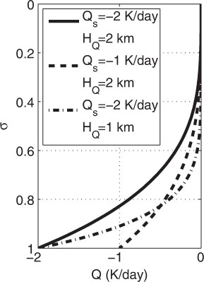
The diabatic cooling rates over the past ice sheets are not known; thus, we can only provide best-guess estimates. Based on reanalysis data, Ringler and Cook (1999) estimated that the diabatic cooling over the surface of the Greenland ice sheet is about Q _s =−2Kd⁻¹ in the present climate (for both summer and winter). The vertical scale of the Greenland cooling was, unfortunately, not specified in Ringler and Cook (1999), but they estimated that the height-scale of the winter cooling over the Rockies is about H _Q =2km. In the light of this, the Q _i profile in Fig. 1 with Q _s =−2Kd⁻¹ and H _Q =2km is used in the coupled simulations in section 5. However, to account for the large uncertainties in Q _s and H _Q , and to understand the physics behind the interactions between diabatic heating and topography over a broader parameter range, simulations with the two additional Q _i profiles in Fig. 1 are conducted in sections 3 and 4.

2.2. Ice sheet model

We use the three-dimensional, land-based ice sheet model SICOPOLIS that treats ice as an incompressible, viscous, non-linear and heat-conducting fluid (Greve, 1997). The model equations are subjected to the shallow-ice approximation, that is, the equations are scaled by a typical aspect ratio (a typical height scaled by a typical length) and only the lowest order terms are kept (Hutter, 1983). It uses Glen's flow law relating the strain rates to the third power of the applied stresses. Ice is simulated in the ‘cold-ice mode’ which means that temperatures above the pressure melting point are artificially reset to the pressure melting temperature. The flow parameters are taken from Greve et al. (1998).

The model is forced by the surface mass balance and the geothermal heat flux. Surface melting is parameterised by the positive degree-day (PDD) method (Braithwaite and Oleson, 1989). Rainfall is assumed to run off the ice sheet immediately, whereas 60% of the annual snowfall is assumed to contribute to the formation of superimposed ice. The degree-day factors are set to 3mmd⁻¹K⁻¹ for snow and 12mmd⁻¹K⁻¹ for ice. The precipitation parameterisation takes the same form as in Roe and Lindzen (2001b) [see their eq. (6)], except for the fact that we set the atmospheric vertical velocity to zero and consequently omit the influence of topographically induced precipitation. The reason for doing this is that we want to isolate the effect of the stationary wave-induced temperature on the surface mass balance of the ice sheet. This implies that the precipitation rate depends only on the saturation water vapour pressure, which is a function of the surface temperature through the Clausius–Clapeyron relation. The amount of total precipitation that comes down as snow depends on the monthly mean surface temperature T _s : If T _s <−10°C (T _s >7°C), all precipitation comes down as snow (rain), and if –10°C<T _s <7°C, the fraction of total precipitation that comes down as rain and snow is linearly interpolated. The geothermal heat flux is set to 55mWm⁻² over the whole domain.

The ice sheet model domain represents a rectangular continent with boundaries at 40°N, 70°N, 130°W and 50°W, which is the same domain used by Roe and Lindzen (2001b). At the continental boundaries, the ice flux divergence is completely balanced by ice berg calving so that the ice thickness is zero. In the absence of ice, the continent is flat except for a 500-m Gaussian topography with boundaries at 63°N, 70°N, 100°W and 120°W. The role of the Gaussian topography is to localise the ice sheet inception. We account for a deformable lithosphere; the bedrock relaxes towards isostatic equilibrium on a timescale of 3kyr. The resolution of SICOPOLIS is set to 1/3°in the horizontal, 81 vertical levels in the ice and 11 levels in the bedrock.

2.3. Surface temperature

The monthly mean surface temperature in SICOPOLIS is given by:5

where T _s0 is the monthly and zonal mean surface temperature in the absence of any surface topography, and t is the time in months. For each month, T _s0 is calculated by time-mean temperature at lowest model level from a 20-yr PUMA simulation without any surface topography, and subsequently extrapolated to the surface using the global-mean lapse rate. The monthly distribution of T _s0 is computed by running PUMA with different values of the restoration temperature difference between the north and the south pole, ΔT _NS. Here, for following values of ΔT _NS are chosen:6

The second term on the rhs of eq. (5) represents a temperature decrease with the height of the ice sheet due to the global-mean lapse rate. The third term represents the stationary-wave-induced temperature anomalies that are given by deviations from the zonal-mean temperature at 950 h Pa. The zonal asymmetries are forced either by the combination of ice-sheet topography and diabatic cooling or by each forcing agent separately. Because most ice-sheet ablation occurs in summer, the temperature anomalies are calculated for mean-summer conditions, that is, ΔT _NS=38K [cf. eq. (6)], but are applied for all the year.

2.4. The coupled model

The atmospheric temperature anomalies T* are interactively computed every 500yr of the ice-sheet simulation. At each coupling event, the height of the ice-sheet surface in SICOPOLIS is bilinearly interpolated to the PUMA grid. The topographically and/or diabatically forced temperature anomalies are then simulated by PUMA and subsequently transformed back to the SICOPOLIS grid with the same bilinear interpolation technique. To decrease the spin-up time at each coupling event, PUMA starts from the last time step in the PUMA simulation at the previous coupling event. Averaging over the last 3.5yr from a 4-yr PUMA simulation with a constant climate forcing (i.e. ΔT _NS=38K) was found to be enough for obtaining a stationary solution.

3. Some theoretical considerations on the interaction between thermal and topographic forcing

In this section, we present some theory on the thermally induced stationary waves and how these interact with the topographical forcing. The analysis provided here about thermal forcing resembles the discussion in Hoskins and Karoly (1981), so the reader is referred to their paper for a more comprehensive discussion. We consider the steady-state thermodynamic equation in cartesian coordinates linearised about a zonal-mean state:7

where z is the vertical coordinate, f is the Coriolis parameter, N the Brunt–Vaisala frequency, ,g the acceleration of gravity, θ₀ a reference potential temperature and u, v and w the zonal, meridional and vertical wind components, respectively. The index ‘h’ indicates that the response is forced only by diabatic heating. The square brackets denote zonal means and the asterisk deviations from the zonal mean. At the surface, the boundary condition for the vertical velocity is:8

where h is the height of the surface topography, , x and y are the zonal and meridional coordinates, respectively and . When and h are non-zero, the wave response is forced both topographically and thermally.

Following the analysis of Hoskins and Karoly (1981), it is found that the vertical advection term of eq. (7) is generally small at midlatitudes; thus, we set w=0 in the subsequent analysis of the thermodynamic balance. We consider eq. (7) in two limits. In the first limit, it is assumed that the heat source is shallow, or equivalently that H _Q ≪H _u , where is the vertical scale of the zonal wind, and is the vertically averaged zonal wind over H _u . Because H _u is about 1–2km at midlatitudes, can be regarded as a representative value of the low-level zonal wind. Thus, in the limit of a very shallow heat source, in eq. (7), the heating is balanced only by zonal advection of potential temperature. The perturbation meridional wind is then given by:9

Equivalently, eq. (9) can be expressed in terms of stream function anomalies ψ^* _h as:10

where L _x is the zonal length scale of the heating anomaly. Equation (10) yields that the stream function response is proportional to both and H _Q , and that the height scale of the response is the same as for the heat source. The potential temperature is given by:11

Thus, linear scaling for a shallow heat source suggests that the potential temperature anomalies should be proportional to H⁻¹ _Q and out-of-phase with the stream function anomalies.

The second limit that we consider is when the heating is deep such that H _u ≪H _Q , or equivalently when . Because the response has the same vertical scale as the heating, the first term of eq. (7) vanishes, and the heating is balanced only by meridional advection of potential temperature. Assuming that is a constant, we obtain that:12

The corresponding streamfunction is given by:13

Note that in the limit of exp(−z/H _Q )→1, the temperature response is expected to be small (θ^* _h ∼ ψ^* _h /H _Q →0). Following Hoskins and Karoly (1981), it can be expected that the weakest perturbation winds should balance the heating. This implies that zonal (meridional) advection dominates if H _Q ≪H _u (H _u ≪H _Q ).

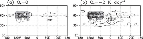
The response of the near-surface stream function and temperature to thermal forcing in our atmospheric model is shown in Fig. 2. Because this study deals with diabatic forcing induced by ice sheets, the results are shown only for parameter combinations representative for thermal cooling (i.e. Q _s <0). The vertical distribution of the cooling in the model is given by eq. (4) and is applied uniformly over the region indicated by the grey shading in Fig. 2.

Fig. 2.  The zonally asymmetric 950 h Pa stream function (panels a, c and e) and temperature (b, d and f) responses to prescribed thermal cooling sources that are given in Fig. (1). The thermal cooling is distributed uniformly over the area given by the grey shading but is zero elsewhere. The employed values of Q _s and H _Q are stated above each panel. The units for the stream funtion and temperature are 10⁶m²s^–1 and K, respectively. Negative values are dotted.

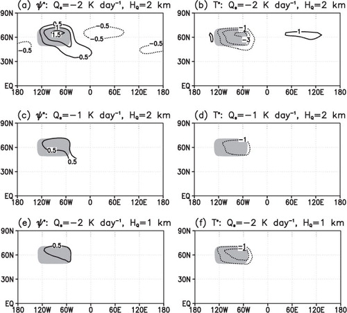
The local stream function response to thermal cooling is a ridge located over the eastern part of the thermal source. This situation allows southerly perturbation winds to prevail over most of the cooling area. Linear theory suggests that the downstream ridge should be shifted 90° relative to the thermal cooling: this can be inferred from eqs (9) and (12). The reason why the ridge is located closer to the cooling area in our simulations is most likely attributed to the presence of thermal damping in the atmospheric model. As suggested by eq. (11), the cooling source yields a negative temperature anomaly that is nearly completely out-of-phase with the stream function. Furthermore, in agreement with linear theory, Fig. 2c, d yields that the amplitude of the near-surface anomaly is roughly proportional to the value of Q _s (compare with panels a and b). Finally, the fact that halving H _Q gives rise to a very similar stream function response as halving Q _s (panels c and e) indicates that the thermal cooling is balanced mainly by zonal advection of potential temperature as suggested by, for example, eq. (10). However, halving H _Q has only a small effect on the temperature response (compare panel b with f). The reason is that ψ^* _h , although reduced, varies over smaller vertical scales [see eq. (11)].

In the presence of topography, eq. (8) yields that the thermally induced perturbation winds have the potential to alter the topographical forcing. A rough estimate of how the strength of the topographical forcing is altered by the heat source can be obtained from linear stationary-wave theory. The linear topographically forced stationary-wave response is typically associated with a ridge (trough) upstream (downstream) of the topography, implying northerly perturbation winds over most of the topography (see Fig. 3a for a linear streamfunction response). Hence, linear theory suggests that the presence of diabatic heating (cooling) over the topography should enhance (reduce) the meridional perturbation winds [cf. eqs (9) and (12)] and consequently increase (decrease) the strength of the topographical forcing.

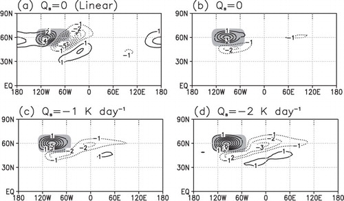
Fig. 3.  The zonally asymmetric stream function response at 950 h Pa to topographic forcing (in 10⁶m²s^–1). The topography is given by eq. (15) and its spatial distribution is indicated by the grey shading. However, the topographic forcing is computed differently for each panel: (a) linear topographic response without any thermal cooling, (b) ‘full’ (linear+non-linear) topographic response without any thermal cooling, (c) full topographic response with a surface cooling on the order of Q _s =−1Kd^–1 and (d) full topographic response with Q _s =−2Kd^–1. In panels b, c and d, the topographical response was computed with the maximum height of topography set to h ₀=2.5km in eq. (15). The linear response in (a) was obtained by running the atmospheric model for 50 model yr (first year discarded as model spin-up) with a lower height of the topography (h ₀=250m). The linear stream function anomalies were thereafter multiplied by a factor 10 to account for the lower topography. In the simulations with thermal cooling (panels c and d), the topographical response was obtained by the difference between the response to both topography and thermal cooling (h ₀=2.5km, Q _s <0) and the response to thermal cooling on a flat surface (h ₀=0, Q _s <0). The vertical distribution of the thermal forcing is given by eq. (4) using H _Q =2km (graphically illustrated in Fig. 1). Horizontally, the thermal forcing is applied uniformly over the topography. Negative values are dotted.

The qualitative analysis of how the low-level thermally induced perturbation winds alter the strength of the topographical forcing, presented above, is in contrast to the results of Ringler and Cook (1999), who found that the topographical forcing is enhanced (reduced) by diabatic cooling (heating). The reasons why their results differ from those of the linear analysis presented here are twofold. First, if thermal damping was included in eq. (7), the associated trough (ridge) downstream the heating (cooling) would be situated closer to the wave source than a quarter of a wavelength: this can be inferred from Fig. 2. Second, if the topographically forced stationary waves have a non-linear character, the downstream trough is reduced, and the near-surface response is associated with a ridge over most of the topograpy (Cook and Held, 1992; Ringler and Cook, 1997) (see Fig. 3b for illustration). Hence, if the topographical response is non-linear, thermal cooling may enhance rather than reduce the topographical forcing.

As a final comment on this topic, the conditions that determine the linearity of the topographical stationary-wave response are briefly discussed. For a more comprehensive discussion, the reader is referred to Ringler and Cook (1997) or, for the implications on ice sheets, to Liakka et al. (2011). The topographical response is linear when the perturbation winds, induced by the topography, are much smaller than the zonal-mean zonal wind. This situation infers that the boundary condition at the surface, which given by eq. (8), can be approximated as:14

This approximation of the topographical forcing is conventionally used in linear stationary-wave models. For example, such a model was used in Roe and Lindzen (2001b) for studying the interactions with ice sheets. However, because linear theory holds only when the perturbation winds are much smaller than [u], a sufficiently high topography will always produce strong enough perturbation winds that destroy the linear response. Thus, for an increasing height of the topography, there will be a transition from a ‘linear’ topographical response (Fig. 3a) to a ‘nonlinear’ response (Fig. 3b). A detailed analysis of the critical height of the topography, at which the transition to a non-linear response occurs, is provided in Ringler and Cook (1997). They found that the linearity of the topographically forced response depends on features that are associated with the atmospheric state and the topography. For example, their study reveals that the response is expected to be more linear when the meridional temperature gradient is large and when the topography is elongated meridionally rather than zonally.

4. Simulations with idealised topography

To examine the interactions between topographically and thermally forced stationary waves in the present atmospheric model, uncoupled simulations with an idealised topography are conducted. The topography is given by:15

where h ₀ is the maximum height of the topography, λ and φ the longitude and latitude, respectively, λ _w (φ _s ) the westernmost longitude (southernmost latitude) and Δλ(Δφ) the zonal (meridional) extent of the topography. Here, the parameter values of eq. (15) are chosen so that the topography crudely mimics the ice sheet in the control simulation (will be shown in the next section); hence, we use h ₀=2.5km, λ _w =130°W, Δλ = 80°, =50°N and φ _s =20°. The thermal cooling is given by eq. (4) and is applied uniformly over the topography. Unless otherwise stated, all simulations are conducted for 20 model years and the first year is discarded as model spin-up.

Figure 3 shows the topographically forced stream function perturbations at 950 h Pa. For a discussion on the linear and non-linear responses in the absence of thermal forcing (panels a and b) the reader is referred to the end of section 3. The effect of thermal cooling on the non-linear topographical response is shown in Fig. 3c, d. These plots were compiled by taking the difference between the stationary-wave response to both topography and thermal cooling, and the response to thermal cooling on a flat surface. To examine the sensitivity of the topographical response to the magnitude of the thermal cooling, the results are presented for Q _s =−1Kd⁻¹ (panel c), and Q _s =−2Kd⁻¹ (panel d). The vertical scale of the cooling is set to H _Q =2km in both cases. In Fig. 3, it is evident that adding thermal cooling over the ice sheet increases the topographically forced stationary-wave response. In particular, the ridge over the topography is amplified and the spatial distribution of the downstream trough is increased. The topographical response to thermal cooling is greater when Q _s =−2Kd⁻¹ than when Q _s =−1Kd⁻¹, whereas the spatial patterns are similar for both cases.

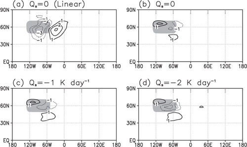
The corresponding temperature anomalies at 950 h Pa are shown in Fig. 4. The linear temperature response (panel a) to topographic forcing is associated with a cold anomaly over most of the topography. Ultimately, the presence of this cold anomaly is the reason why the ice sheets increase their size when interacting with the linear stationary waves (Roe and Lindzen, 2001a, 2001b; Liakka and Nilsson, 2010; Liakka et al., 2011). When the topographical response is non-linear, the temperature anomalies have a completely different pattern compared to the linear case (panel b). In the non-linear regime, the cold anomaly is reduced and displaced towards the northeast, whereas the warm anomaly is found over the northwestern parts of the topography. The fact that the largest temperature anomaly in the non-linear simulation is found over the northern slope of the topography implies that its effect on ice-sheet evolution through changing the ablation is very small (see the next section; Liakka et al. 2011). Adding thermal cooling to the non-linear topographical response serves to increase the spatial distribution and strength of the cold anomaly: the effect of increasing surface cooling on the topographically forced temperature response is that the cold anomaly expands towards the southwest (panels c and d).

Fig. 4.  Same as Fig. 3 but for the zonally asymmetric temperature (in K) at 950 h Pa.

The enhanced cooling over the topography, arising from the non-linear interaction between thermal and topographical forcing, is caused by the perturbation winds that are enhanced by thermal cooling (Fig. 3c, d). This is illustrated in Fig. 5, which shows the topographically forced perturbation winds that arise from thermal cooling together with the near-surface temperature from the non-linear simulation with topography and no thermal forcing. Fig. 5 yields that the increased anticyclonic circulation, induced by thermal cooling, serves to increase the cold-air advection over the eastern and southern parts of the topography. The fact that the advection is stronger when Q _s =−2Kd⁻¹ compared to when Q _s =−1Kd⁻¹ explains why the topographically forced cold anomaly in Fig. 4 becomes larger for a stronger surface cooling. Possibly, also other features, for example, interactions between the topographically forced perturbation winds and temperature anomalies induced by thermal forcing, or changes in the mean flow when introducing topography, could change the thermally modified temperature response in Fig. 4. However, in the present model, the effects of these features are small compared to the effect of increasing advection through changes in the perturbation winds (not shown).

Fig. 5.  Vectors: the difference of the topographically forced perturbation winds (in ms⁻¹) at 950 h Pa between the simulation with both topographical and thermal forcing (h ₀=2.5km, Q _s <0) and the simulation with topographical forcing in isolation (h ₀=2.5km, Q _s <0). The topographical response was computed with (a) Q _s =−1Kd⁻¹ and (b) Q _s =−2Kd⁻¹. Contours: temperature (in K) at 950 h Pa in the simulation with topography and no thermal forcing. The spatial extent of the topography is given by the grey shading.

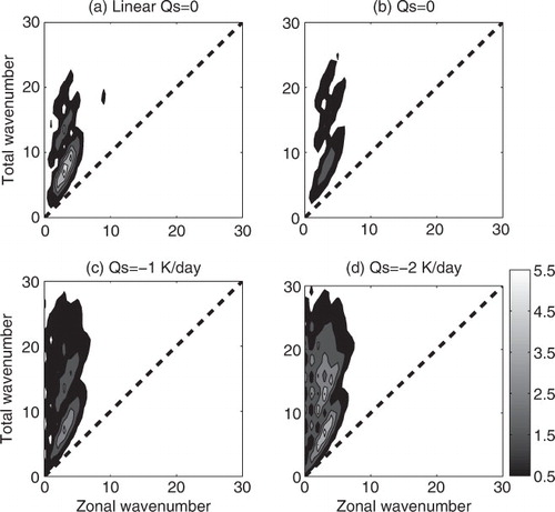
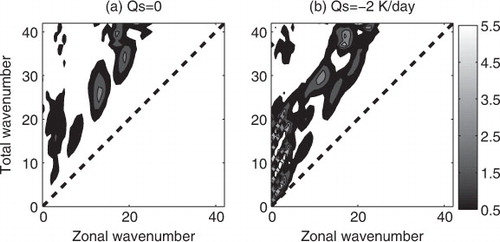
To examine why the topographical response is amplified by thermal cooling as suggested in Fig. 3, we consider the power spectrum of the topographical forcing (eq. 8) for all the simulations in Fig. 3. The power spectrum shows the relative energy contribution by each spectral coefficient in the triangularly truncated atmospheric model. The results are shown in Fig. 6. In the absence of thermal forcing, the linear approximation [Eq. (14)] yields a substantially stronger stationary-wave forcing than when using the full representation of the forcing (panels a and b). This explains why the amplitude of the linear response in Fig. 3 is much larger than of the non-linear response. Figure 6c, d yields that the topographical forcing is amplified by the presence of thermal cooling. This is the reason why the topographically forced response increases when adding thermal cooling, and ultimately, why thermal cooling amplifies the topographically forced cold anomaly. The fact that thermal cooling yields a strengthening rather than a weakening of the topographical forcing is linked to thermal responses in Fig. 2. Locally over the topography, the near-surface stream function response to thermal cooling is similar to the non-linear topographical response in Fig. 3b. Hence, the topographically forced perturbation winds that contribute to the topographical forcing through eq. (8) should be enhanced by the perturbation winds induced by thermal cooling.

Fig. 6.  The power spectrum of the topographical forcing in the simulations with idealised topography [eq. (15): h ₀=2.5km]. In panel (a) the forcing was obtained by eq. (14) that is conventionally used in linear models. In all other panels, the power spectrum of the full topographical forcing, as given by eq. (8), is shown for the following values of the surface cooling (b) Q _s =0, (c) Q _s =−1Kd^–1and (d) Q _s =−2Kd^–1. When calculating the power spectrum, the winds at 950 h Pa were used and w was set dimensionless using the planetary radius (6370km) and the rotational frequency of the Earth (7.29×10^–5s^–1). The values have been further scaled by 10^–15. The dashed line represents the truncation of the model. The topographical forcing is very small for the highest wavenumbers, while only the 30 lowest wavenumbers are shown.

5. Coupled simulations

In this section, it is examined how the effect of thermal cooling on the topographically forced stationary-wave response influences the evolution of ice sheets. We have performed three simulations with the coupled atmosphere ice-sheet model (see section 2.4): (1) a ‘control’ simulation in which the ice sheet evolves in a constant zonally symmetric climate without any influence of stationary waves [i.e. T* = 0 in eq. (5)], (2) a simulation with topographically forced stationary waves but with no thermal cooling (Q _s=0) and (3) a simulation in which the topographically forced stationary waves are computed with thermal forcing. The topographical simulation (2) is shown also in Liakka et al. (2011), so the reader is referred to their paper for a wider discussion on that simulation. In the thermal-topographical simulation (3), we use the same representation of the thermal forcing as in the uncoupled simulations with Q _s=−2Kd⁻¹ and H _Q =2km.

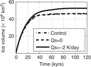
The time evolution of the ice sheet for the three simulations is shown in Fig. 7. The simulated ice volumes obtained with prescribed zonally symmetric temperature and with coupled topographically forced stationary waves are essentially identical: the ice volume amounts to 46×10⁶km³ at equilibrium. Including thermal forcing in the coupled simulation increases the equilibrium ice volume to 53×10⁶km³.

Fig. 7.  The time evolution of the ice sheet in the three ice-sheet simulations conducted in this study. In the control simulation (dashed-dotted line), there are no stationary waves, i.e. T* = 0 in eq. (5) and the climate is zonally uniform. In the ‘Q _s =0’ simulation (dashed line), the stationary waves are topographically forced but the thermal cooling induced by the ice sheet is set to zero. In the ‘Q _s =−2Kd^–1’ simulation (solid line), thermal cooling (given by the solid line in Fig. 1) was added to the topographical forcing. The thermally modified topographical response was computed as follows: First, a simulation was performed both with topography and thermal cooling that were distributed uniformly over the ice-sheet area. Second, another simulation was conducted with the same properties of the thermal cooling field but with no topography (h=0). Finally, the topographically forced response was obtained by taking the difference of the temperature anomalies between the two simulations.

The equilibrium ice thickness in the three simulations is shown in Fig. 8 together with the temperature anomalies at 950 h Pa. In the control simulation, the ice sheet is zonally uniform as expected. When forced by topographically forced stationary waves in isolation, the shape of the equatorward margin of the ice sheet is nearly identical to the one in the control simulation. The reason why the topographically forced stationary waves have very weak effect on the equilibrium shape of the ice sheet is that the associated temperature anomalies are located along the northern ice-sheet slopes, where the ablation is negligible due to cold conditions even in summer. In turn, the unfavourable location of the temperature anomalies for affecting ice-sheet ablation is associated with the non-linearity of the stationary-wave response. For a further discussion of the interactions between the topographically forced waves and ice sheets, see Liakka et al. (2011).

Fig. 8.  The ice thickness (in km; filled contours) and the topographically forced temperature anomalies (in K; coloured contours) at 120kyr in (a) the control, (b) ‘Q _s =0’ and (c) ‘Q _s =−2Kd^–1’ simulations.

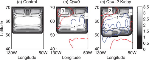
As noted before, the presence of thermal cooling increases the nonlinear topographically forced stationary-wave response. Fig. 8c illustrates that this feature causes the ice sheet to advance further equatorward, especially near the continental west coast. The increased extent is linked to an enhanced cooling over the equatorward slope of the ice sheet. The physics behind the equatorward expansion of the cold anomaly was analysed in connection with the uncoupled simulations in the previous section: the amplified topographical stationary-wave response, which arises from the non-linear interactions with thermal cooling, is associated with an enhanced cold-air advection over the eastern and southern parts of the ice sheet (Fig. 5). Ultimately, the increased advection of cold air gives rise to a larger cold anomaly (Fig. 4d). However, while the cold anomaly in Fig. 4d is located over the southeastern parts of the topography, the cold anomaly in the coupled simulation in Fig. 8c expands all the way to the westernmost parts of the ice sheet.

To reveal further insight into the different temperature responses in the coupled and uncoupled simulations, the stream function anomalies from both coupled simulations are shown in Fig. 9. The spatial patterns of the stream function anomalies in the coupled simulations are very similar to the ones simulated with idealised topography (Fig. 3b, d). However, the amplitude of the stream function response is greater in the coupled simulations. Because the stationary waves in both the coupled and uncoupled simulations have been compiled with identical model parameters, the amplified stream function response in the coupled simulations must be ascribed to the ice-sheet topography and the spatial distribution of the thermal cooling. Because the maximum height of the topographies in the coupled and uncoupled simulations are roughly the same (about 2.5 km), the increased response in the coupled simulations is, thus, caused by the steeper slopes of the ice-sheet topography.

Fig. 9.  Same as in Fig. 3b, d, but with the equilibrium ice-sheet topography (i.e. the ones in Fig. 8b, c) imposed at the lower boundary of the atmospheric model.

That the steeper slopes of the ice-sheet topography are responsible for the amplified response in the coupled simulations is confirmed in Fig. 10 that shows the power spectrum of the topographical forcing induced by the equilibrium ice sheets in Fig. 8. The results in Fig. 10a and b should be compared with Fig. 6b and d, respectively. Relative to the idealised topography in the uncoupled simulations, the presence of ice-sheet topography generally increases the topographical forcing of stationary waves. This explains the enhanced stream function response in Fig. 9 compared with that in Fig. 3d as well as the increased expansion of the cold anomaly in Fig. 8c towards the west compared with that in Fig. 4d. Another feature that is clearly evident in Fig. 10 is that also higher wavenumbers of the atmospheric model contribute to the topographical stationary-wave forcing. The explanation is due to the steep ice-sheet slopes and the small-scale structures of ice-sheet topography that require much higher wavenumbers in the atmospheric model to be resolved.

Fig. 10.  Same as Fig. 6b, d, but with the equilibrium ice-sheet topography (i.e. the ones in Fig. 8b, c) was used in the calculation of the topographical forcing. In contrast to Fig. 6, however, the topographical forcing is shown for all the wavenumbers in the atmospheric model.

6. Summary and conclusions

In this study, coupled atmosphere-ice sheet simulations have been conducted to examine interactions between stationary waves and ice sheets. This work can be regarded as a continuation of the previous studies on the stationary wave-ice sheet interactions undertaken by Roe and Lindzen (2001b) and Liakka et al. (2011). Similar to these studies, this work has analysed how the stationary waves have influenced the equilibrium features of a single ice sheet through the zonal variations of temperature. However, in Roe and Lindzen (2001b) and Liakka et al. (2011), the stationary waves were induced only by the ice-sheet topography, whereas other stationary-wave forcing agents, such as zonal variations of diabatic heating, were not considered. This study has focused on how the topographically forced stationary waves are influenced by ice-sheet-induced thermal cooling of the atmosphere.

In isolation, the effect of topographically forced stationary waves on the ice-sheet extent is very weak. The reason is that the stationary-wave response is non-linear implying that the largest temperature anomaly is located along the northern ice-sheet slope where the ablation is negligible. When ice-sheet-induced thermal cooling is added to the topographical forcing, the associated stationary waves serve to increase the equatorward extent of the ice sheet. The underlying physics is that thermally induced perturbation winds increase the topographical forcing of stationary waves through the topographically forced vertical velocities. Ultimately, this feature yields an amplified stream function response that is associated with an increased advection of cold air over the ice sheet. Hence, in agreement with Ringler and Cook (1999), this study reveals a strong non-linear interaction between thermal and topographical forcing, in which topographical forcing is substantially enhanced by thermal cooling. However, to the knowledge of the present author, this is the first study that considers the implications of these non-linear interactions on the ice-sheet evolution.

In the coupled simulation conducted here, the stationary-wave-induced temperature anomalies that arise from the non-linear interactions between thermal and topographical forcing yield an east–west asymmetry of the ice sheet. At equilibrium, the equatorward ice-sheet extent gradually increases towards the west, and the maximum extent is obtained near the continental west coast. This shape of the ice sheet is caused by a cold anomaly that expands from the eastern part of the ice sheet towards the southwestern margin. However, the exact location of this cold anomaly is sensitive to some of the employed model parameters. For example, it is found that southwestward expansion of the cold anomaly over the ice sheet increases with the magnitude of the prescribed surface cooling over the ice sheet. This result can possibly yield some insight into why the different atmospheric models in, for example, Charbit et al. (2007) gave rise to such different shapes of the LGM ice sheets.

The present results suggest that the high albedo of the snow surface of ice sheets should increase the amplitude of the stationary waves, not only directly through diabatic cooling but also indirectly through the non-linear interactions with topographical forcing. Hence, the interactions between thermal and topographical forcing should serve to increase the sensitivity of the stationary-wave response to changes of the ice-sheet albedo. In glacial conditions, one potential candidate for changing the albedo of the snow surface of ice sheets is deposition of dust. Analyses from ice cores have revealed that glacial conditions are generally associated with larger atmospheric dust concentrations (Mahowald et al., 1999). Calov et al. (2005) estimated that the increased dust concentrations at LGM reduced the albedo of snow by 10%–30%. Hence, the present results suggest the possibility that the larger dust concentrations at LGM weakened the topographically forced stationary waves through reducing the albedo of the ice sheets. The impact of the dust deposition on the circulation is hinted in Colleoni et al. (2009), who investigated the influence of dust deposition on snow on the surface mass balance of the Eurasian ice sheet at the Late Saalian Maximum (about 140 kyr ago).

In this study, the atmospheric model lacks a representation of moisture, which also constitutes a diabatic forcing agent of the stationary waves. Potentially, localised precipitation anomalies along the margins of the ice sheet could alter the topographical forcing and the associated stationary-wave response. However, except near the ice-sheet margins, the local climate over continental-scale ice sheets is generally associated with dry conditions (Yamagishi et al., 2005). Furthermore, ice sheets have complex geometry, and the relatively low resolution of the atmospheric model used in this study may neglect small-scale structures of the ice-sheet topography that are relevant for an appropriate representation of the topographical forcing. When ice-sheet topography is imposed to the atmospheric model, even the highest spectral wavenumbers are activated to describe the topography. At these small scales, features associated with numerics, such as hyperdiffusion, become important.

The main result of this article is that thermal cooling, induced by ice sheets, substantially amplifies the non-linear topographical stationary-wave response. Using plausible parameter values of the thermal cooling, it is shown that the topographically forced stationary-wave amplitudes can well be doubled as a result of thermal cooling. It is suggested that the non-linear interactions between thermal and topographical forcing is highly significant and should preferably be considered for a satisfactory treatment of the mutual interactions between stationary waves and ice sheets.

7. Acknowledgements

The author is grateful to Johan Nilsson for his valuable comments on the manuscript. The work reported here was supported by the Swedish Research Council and the Climate Research School at Stockholm University and is a contribution from the Bert Bolin Centre for Climate Research.

References

- Abe-Ouchi A. Segawa T. Saito F. Climatic conditions for modelling the Northern Hemisphere ice sheets throughout the ice age cycle. Clim. Past. 2007; 3: 423–438.
- van den Berg J. van de Wal R. Oerlemans J. Mass balance model for the Eurasian ice sheet for the last 120,000 years. Global Planet. Change. 2008; 61: 194–208.
- Berger A. Long-term variations of caloric insolation resulting from the Earth's orbital elements. Quat. Res. 1978; 9: 139–167.
- Berger A. Loutre M. F. Galle H. Sensitivity of the LLN climate model to the astronomical and CO2 forcings over the last 200 ky. Clim. Dyn. 1998; 14: 615–629.
- Bonelli, S, Charbit, S, Kageyama, M, Woillez, M.-N, Ramstein, G and co-authors. 2009. Investigating the evolution of major Northern Hemisphere ice sheets during the last glacial-interglacial cycle. Clim. Past. 5, 329–345.
- Braithwaite, R. J and Oleson, O. B. 1989. Calculation of glacier ablation from air temperature, West Greenland. In: Glacier Fluctuation and Climate Change. J. Oerlemans. Kluwer Academic, Dordrecht, 219–233.
- Calov R. Ganopolski A. Claussen M. Petoukhov V. Greve R. Transient simulation of the last glacial inception. Part i: glacial inception as a bifurcation in the climate system. Clim. Dyn. 2005; 24(6): 545–561.
- Charbit S. Ritz C. Philippon G. Peyaud V. Kageyama M. Numerical reconstructions of the Northern Hemisphere ice sheets through the last glacial-interglacial cycle. Clim. Past. 2007; 3: 15–37.
- Clark P. U. Mix A. C. Ice sheet and sea level of the last glacial maximum. Quat. Sci. Rev. 2002; 21: 1–7.
- Claussen, M, Fohlmeister, J, Ganopolski, A., and Brovkin, V. 2006. Vegetation dynamics amplifies precessional forcing. Geophys. Res. Lett. 33((9)):, L09709, 10.3402/tellusa.v64i0.11088.
- CLIMAP. 1984. The last interglacial ocean. Quat. Res. 21, 123–224.
- Colleoni F. Krinner G. Jakobsson M. Peyaud V. Ritz C. Influence of regional parameters on the surface mass balance of the Eurasian ice sheet during the peak Saalian (140 kya). Global and Planet. Change. 2009; 68: 132–148.
- Colleoni, F, Liakka, J, Krinner, G, Jakobsson, M, Masina, S and co-authors. 2010. The sensitivity of the Late Saalian (140ka) and LGM (21ka) Eurasian ice sheets to sea surface conditions. Clim. Dyn. 37, 1–23. 10.3402/tellusa.v64i0.11088.
- Cook K. H. Held I. M. The stationary response to large-scale orography in a general circulation model and a linear model. J. Atmos. Sci. 1992; 49: 525–539.
- Dyke, A. S. 2004. An outline of North American deglaciation with emphasis on central and northern Canada. In: Quaternary Glaciations-Extent and Chronology, Part II. Vol. 2bJ. Ehlers and P. L. Gibbard. Elsevier, Amsterdam, 373–424.
- Dyke, A. S, Andrews, J. T, Clark, P. U, England, J. H, Miller, G. H and co-authors. 2002. The laurentide and innuitian ice sheets during the last glacial maximum. Quat. Sci. Rev. 21(1–3), 9–31. 10.3402/tellusa.v64i0.11088.
- Fraedrich, K, Lunkeit, F and Kirk, E. 1998. PUMA: portable university model of the atmosphere. Technical Report 16. Deutsches Klimarechenzentrum. 38.
- Greve R. Application of a polythermal three-dimensional ice sheet model to the Greenland ice sheet: response to steady-state and transient climate scenarios. J. Climate. 1997; 10: 901–918.
- Greve R. Weis M. Hutter K. Palaeoclimatic evolution and present conditions of the Greenland ice sheet in the vicinity of summit: an approach by large-scale modelling. Paleoclimates. 1998; 2(2–3): 133–161.
- Hall M. N. J. Valdes P. J. Dong B. The maintenance of the last great ice sheets: a UGAMP GCM study. J. Climate. 1996; 9: 1004–1019.
- Hoskins B. J. Karoly D. J. The steady linear response of a spherical atmosphere to thermal and orographic forcing. J. Atmos. Sci. 1981; 38: 1179–1196.
- Hoskins B. J. Simmons A. J. A multi-layer spectral model and the semi-implicit method. Quart. J. Roy. Meteor. Soc. 1975; 101: 637–655.
- Hutter, K. 1983. Theoretical Glaciology: Material Science of Ice and the Mechanics of Glaciers and Ice Sheets. D. Reidel, Dordrecht, 510.
- James I. N. Gray L. J. Concerning the effect of surface drag on the circulation of a baroclinic planetary atmosphere. Quart. J. Roy. Meteor. Soc. 1986; 112: 1231–1250.
- Kageyama, M, Laine, A, Abe-Ouchi, A, Braconnot, P, Cortijo, E and co-authors. 2006. Last Glacial Maximum temperatures over the North Atlantic, Europe and western Siberia: a comparison between PMIP models, MARGO sea-surface temperatures and pollen-based reconstructions. Quat. Sci. Rev. 25(17–18), 2082–2102.
- Källén E. Crafoord C. Ghil M. Free oscillations in a climate model with ice-sheet dynamics. J. Climate. 1979; 36: 2292–2303.
- Kleman, J, Jansson, K, De Angelis, H, Stroeven, A. P, Hättestrand, C and co-authors. 2010. North American ice sheet build-up during the last glacial cycle, 115–321 kyr. Quat. Sci. Rev. 29, 2036–2051.
- Liakka J. Nilsson J. The impact of topographically forced stationary waves on local ice-sheet climate. J. Glac. 2010; 56: 534–544.
- Liakka, J, Nilsson, J., and Löfverström, M. 2011. Interactions between stationary waves and ice sheets: linear versus nonlinear atmospheric response. Clim. Dyn. 10.3402/tellusa.v64i0.11088.
- Lindeman M. Oerlemans J. Northern Hemisphere ice sheets and planetary waves: a strong feedback mechanism. Int. J. Clim. 1987; 7: 109–117.
- Mahowald, N, Kohfeld, K, Hansson, M, Balkanski, Y, Harrison, S. P, Prentice, I. C, Schulz, M., and Rodhe, H. 1999. Dust sources and deposition during the last glacial maximum and current climate: a comparison of model results with paleodata from ice cores and marine sediments. J. Geophys. Res. 104, 15895–15916. 10.3402/tellusa.v64i0.11088.
- Milankovitch M. Mathematische klimalehre und astronomische theorie der klimaschwankungen i [Mathematical climate and astronomical theory of climate fluctuations]. Handbuch der klimatologie, Part A. Kppen W.Geiger R.Gebruder Borntreger: Berlin, 1930; 1–176.
- Oerlemans J. Model experiments on the 100,000-yr glacial cycle. Nature. 1980; 287: 430–432.
- Paul, A and Schaefer-Neth, C. 2003. Modeling the water masses of the atlantic ocean at the Last Glacial Maximum. Paleoceanography. 18((3)):, 1058, 10.3402/tellusa.v64i0.11088.
- Ringler T. D. Cook K. H. Factors controlling nonlinearity in mechanically forced stationary waves over orography. J. Atmos. Sci. 1997; 54: 2612–2629.
- Ringler T. D. Cook K. H. Understanding the seasonality of orographically forced stationary waves: Interaction between mechanical and thermal forcing. J. Atmos. Sci. 1999; 56: 1154–1174.
- Roe G. H. Orographic precipitation. Ann. Rev. Earth Planet. Sci. 2005; 33: 645–671.
- Roe G. H. Lindzen R. S. A one-dimensional model for the interaction between continental-scale ice sheets and atmospheric stationary waves. Clim. Dyn. 2001a; 17: 479–487.
- Roe G. H. Lindzen R. S. The mutual interaction between continental-scale ice sheets and atmospheric stationary waves. J. Climate. 2001b; 14: 1450–1465.
- Sanberg J. A. M. Oerlemans J. Modeling of Pleistocene European ice sheets: the effect of upslope precipitation. Geol. Mijnbouw. 1983; 62: 267–273.
- Shackleton N. J. The 100,000-year ice-age cycle identified and found to lag temperature, carbon dioxide, and orbital eccentricity. Science. 2000; 289: 1897–1902.
- Tarasov L. Peltier W. R. Terminating the 100 kyr cycle. J. Geophys. Res. 1997; 102: 21665–21693.
- Weertman J. Milankovitch solar radiation variations and ice age ice sheet sizes. Nature. 1976; 261: 17–20.
- Yamagishi T. Abe-Ouchi A. Saito F. Segawa T. Nishimura T. Re-evaluation of paleo-accumulation parameterization over Northern Hemisphere ice sheets during the ice age examined with a high-resolution AGCM and a 3-D ice-sheet model. Ann. Glaciology. 2005; 42: 433–440.