Global gridded dataset of lake coverage and lake depth for use in numerical weather prediction and climate modelling

ABSTRACT

A global dataset of lake coverage and lake depth was developed for use in numerical weather prediction and climate modelling. It provides the global gridded information on lake depth with the resolution of 30 arc sec. (approximately 1 km). It was obtained by mapping data on mean lake depth for ca. 13 000 freshwater lakes. Apart from the mean depth, the bathymetry for 36 large lakes is included. Information for individual lakes was collected from regional databases, water cadastres and public sources. For mapping, the land cover map ECOCLIMAP2 was used. A new automatic probabilistic mapping method was developed and is described here. We discuss also how to project the lake depth data onto the numerical atmospheric model grid and how to achieve the consistency of physiographic datasets when several maps are used in a model.

• parameterization of lakes
• surface processes
• physiographic data

1. Introduction

The atmospheric boundary layer regime, turbulent fluxes and radiation fluxes depend strongly on surface processes. Each type of surface with their specific features should be represented in an atmospheric model. In regions with high percentages of the lake area, such as Canada, the Scandinavian Peninsula, Finland, the European part of northern Russia or Siberia, lakes affect local weather conditions and the climate at the regional scale (Eerola et al., 2010; Samuelsson et al., 2010). Lakes can potentially have a noticeable influence on the global climate through carbon emissions (Tranvik et al., 2009) and, for thermokarst lakes, methane emissions (Walter et al., 2007). In regions with low percentage of lakes, their impact is less pronounced, but their local influence is not negligible. Besides, even for small lakes we must provide the model with some reasonable information about their state, at least not to introduce gross errors. With increase in the atmospheric model horizontal resolution, the local coverage of lakes also increases. Observations of the lake surface temperate and ice coverage are not yet being assimilated in numerical weather prediction (NWP) models, this makes the problem pressing. To account for lakes, atmospheric models need to be coupled with specific lake models that calculate surface fluxes depending on the state of lakes. Being coupled with an atmospheric model, a lake model runs in every ‘lake’ grid box of an atmospheric model domain. If a mosaic approach is used, with every grid box fractionally covered by different surface types, it will run in every grid box with non-zero lake fraction.

To run lake models, databases with gridded lake parameters are needed. First and foremost, we need the lake coverage given by a map. The map can be provided in the form of a binary mask, or in the form of a lake fraction field (the lake fraction is the percentage of the grid box covered by lake water). The most important parameters are the lake depth and the turbidity. The lake depth influences the heat storage in the lake, whereas the turbidity modifies the vertical profile of the absorption of the solar radiation. The lake depth is strictly needed by any lake model. All these parameters are available from hydrological studies, but usually only for individual lakes. They are seldom represented on a map. The data available for individual lakes usually include the lake area, the mean lake depth, the maximum lake depth, the lake climatology and the chemical, biological and socio-economical characteristics of lakes. For global and regional atmospheric numerical models, fields of lake parameters must be global and must contain information about all lakes on the map. The characteristic scale of meteorological applications is several kilometres, so less fine data than in hydrology are satisfactory. A major constraint is to estimate parameters at the global scale, even if rough estimations are to be made. Maps give the details of geographical location of lakes but normally provide very few information about their parameters. The most appreciable map developed specially for inland water bodies is the Global Lakes and Wetlands Database (GLWD) (Lehner and Döll, 2004). Non-special land cover maps, such as Global Land Cover Characteristics dataset (GLCC) (Loveland et al., 2000), the ECOCLIMAP dataset (Masson et al., 2003) and others also contain information about lakes, these maps are global.

First dataset combining information for individual lakes with a map was developed by Kourzeneva (2010). But in that product, the mapping algorithm was designed to operate with a limited area, so it was applicable only for regional models. Only the mean lake depth was provided, with no bathymetry included, not even for large lakes. The idea to consider random errors of the map and of coordinates of lakes was used in the mapping procedures. However, the mapping method itself was rather intuitive and quite simple, it applied elementary scanning search algorithm.

The objective of the present work is to facilitate the progress in this direction continuing the work of Kourzeneva (2010) to develop a global gridded dataset of lake-related parameters for use in numerical atmospheric modelling. The new dataset represents global lake depth information on the fine grid with the resolution of 30 arc sec. (approximately 1 km). Information in gridded form is customary for the atmospheric modelling community and gives the possibility to use it for global models. The new dataset contains data for more individual lakes. As a result of inter-comparison of different land-use datasets, ECOCLIMAP2 (Champeaux et al., 2004) was chosen for mapping. For large lakes, the bathymetry was included. We developed a novel mapping method that is much more complicated and better justified mathematically, solving an optimisation problem for search algorithm. Section 2 describes the lake map, in Section 3 we treat lake depth, including the data for individual lakes and the new mapping method. Section 4 describes the algorithm for the projection of the data on various model grids and the problem of the consistency between different maps and different grids. Finally, limitations of the present database and perspectives are discussed in the last two sections.

2. Lake mapping

During the last two decades, many projects devoted to the development of global and regional land cover datasets were launched. Among them, the most significant examples are GLCC, ECOCLIMAP, GLC2000 (Bertholomeé and Belward, 2005), CORINE (CEC, 1993) and GlobCover (Bicheron et al., 2006). Many of them are used for mapping, to specify physiographic fields for atmospheric models. Maps can be provided in a vector or raster form. In atmospheric modelling, the raster form of a map is preferable, with pixels classified in different land surface types according to the legend. These land cover datasets can be used for lake mapping as well. GLWD dataset, designed specially to map inland water bodies, and water masks used in remote sensing are also applicable. To discriminate lakes, the definition ‘inland water’/‘no inland water’ (or similar) is used. But the classification differs between maps: GLC2000 does not distinguish between ocean water and lake water, whereas GLCC, GLWD and ECOCLIMAP classify separately seas, lakes and rivers. Note that rivers are recognised quite poorly by all land cover datasets, and very often they are mixed up with lakes. The products have different resolutions, from 25 m for CORINE to 1 km for GLCC, ECOCLIMAP, GLC2000 and GLWD. When the grid size of a numerical atmospheric model is larger, the lake fraction can be easily calculated from these land cover datasets in a standard way.

Most of these maps are not independent. They are compiled using the same basic information, for example, the Digital Chart of the World (ESRI, 1993), the ArcWorld 1:3M dataset (ESRI, 1992) and Shuttle Radar Topography Mission Water Body Dataset (Farr et al., 2007). Hence, all kinds of errors and inaccuracies, including those for the shoreline are inherited from one map to another. This problem was discussed in the literature (Lehner and Döll, 2004; Kourzeneva, 2009; Merchant and MacCallum, 2009; Kourzeneva, 2010). There are two types of errors: small, ‘random’ errors and gross errors. The illustration of shoreline ‘random’ errors is given by Fig. 1 with four different maps for the territory, including Lake Saimaa (Finland). All maps have the same resolution of 1 km, but the lake shoreline varies between maps. Using this resolution only, we can neither fix these errors, nor say which map is more accurate and more likely the truth. To estimate accuracy and to correct maps could be possible only from finer resolution data (allowing them to contain random errors also). For example, very high resolution remote sensing images could be helpful. For the atmospheric model lake fraction field, these relatively small coastline ‘random’ errors are not very important, although they may produce a bias on the actual inland water area. But when combining a map with information for individual lakes, these errors may appear to be a key point. Gross errors are illustrated by lack of the island Isle Royale (the surface area is 535 km²) on Lake Superior in the first version of ECOCLIMAP, or by lack of Lake Toba (the surface area is 1130 km²) in this dataset. It is quite easy to fix these errors, and they must be fixed when observed.

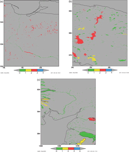
Fig. 1.  Shoreline in Lake Saimaa region in southern Finland given by different raster maps: (a) GLCC, (b) GLWD, (c) ECOCLIMAP (v. 1), (d) ECOCLIMAP (v. 2). Dark blue colour is lake water, yellow colour is land. The resolution (the pixel size) of all maps is 30 arc sec.

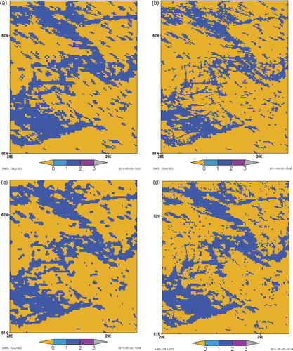
To choose a basic map for mapping, we performed an expert-based inter-comparison of different land cover datasets. We examined only global products with 1 km resolution containing ‘inland water’ land surface type, namely GLCC, GLWD and two versions of ECOCLIMAP – ECOCLIMAP and ECOCLIMAP2 (Champeaux et al., 2004). ECOCLIMAP2 is an improvement of ECOCLIMAP over a domain encompassing Europe (11 °W to 62 °E in longitude, 25 °N to 75 °N in latitude). ECOCLIMAP2 uses the version 8 of CORINE land cover map for the year 2000 and the GLC2000 for the rest of this area. These maps were visually compared with remote sensing images, testing several regions on different continents. Well-known lakes were observed, giving the main attention to Europe. Territories with potential uncertainties and gross errors, such as Lake Chad, Lake Toba, Aral Sea, basins of big rivers, were also considered. A total of 40 regions were investigated. For these test regions, ECOCLIMAP2 had the smallest biases, although several gross errors were found. It has been decided to choose ECOCLIMAP2 for lake mapping. An important practical argument for this choice was that ECOCLIMAP2 is widely used in NWP and climate modelling, and thus less consistency problems will appear in the future. All observed gross errors were fixed using information from other land cover datasets.

3. Lake depth

3.1. Depth data for individual lakes

Mean lake depth information for individual lakes was collected from different regional databases, water cadastres and public sources. For Europe, data were kindly provided by different organisations, mainly through personal communications. The process of collecting and processing data for Europe is described in details in Kourzeneva (2010). For the rest of the world, data were picked up from different public sources on the internet. Many data from Wikipedia were used. Although Wikipedia is a ‘semi-scientific’ source of information and provides no legal warranty, for practical reasons we did not reject these data. First argument for this is that even rough estimates are helpful and better than nothing. Second, Wikipedia national pages are constantly very rich, and being too strict we lose much information. Third, in Wikipedia, information from scientific and governmental institutions around the world is normally used, and most of pages contain references to the appropriate public sources or literature. But to follow all these links and literature references and to contact all these institutions and organisations directly is very time consuming. Thermodynamically, the behaviour of natural and man-made lakes is similar. Hence, we did not distinguish between natural and artificial lakes and included information on both types in the database. For each particular lake, the following information was collected and kept in the dataset for individual lakes: the geographical coordinates, the mean depth, the maximum depth, the surface area, the lake name and the name of the country where the lake is located. Geographical coordinates of the lake were defined by coordinates of an arbitrary point of its water surface. By now, the dataset for individual lakes comprises ca. 13 000 freshwater lakes, the list of references includes ca. 295 items. Metadata are located together with data.

Saline lakes and endorheic basins behave differently from freshwater lakes. Many of them are not permanent, their surface area and shape may change over time. Some of them are intermittent or ephemeral. They can hardly be simulated by freshwater lake models, particularly by simplified lake models used in numerical atmospheric modelling to represent lakes. Saline lakes are separated, and information for them is kept in an additional dataset. Brackish lakes with low salinity (<10‰) and with the stable surface area behave more similar to freshwater lakes, so they are not separated from them. The additional dataset for saline lakes comprises ca. 220 saline lakes and endorheic basins.

3.2. Bathymetry data for large lakes

For large lakes covering several grid boxes of an atmospheric model, information about the bathymetry is useful. Being provided with bathymetry information, a 1D lake model may run in every atmospheric model grid box over the large lake using specific lake depth. This makes it possible to reproduce the surface temperature patterns for large lakes. In principle, the bathymetry may be obtained from different kinds of maps in graphic form: from topographic and navigation maps or from sketch-maps of different atlases. In addition, gridded information from global sea bathymetry datasets is available, as far as they may contain information for some large lakes also. By now, there are two global sea bathymetry datasets widely used in different applications: ETOPO5 (ETOPO5, 1988) and ETOPO1 (Amante and Eakins, 2009) with its previous version, ETOPO2. For lakes, ETOPO1 contains detailed information about the bathymetry of the American Great Lakes with a resolution of 1 arc min. ETOPO5 contains the bathymetry for some other large lakes at a resolution of 5 arc min, but this dataset was not used due to its poor quality. Information for other large lakes is only available from graphic maps and hence needs digitising.

As digitising is time consuming, a selection of lakes has been made. For this version of the database, only lakes that cannot be characterised by their mean depth in models were treated. In the case of deep lakes (deeper than approximately 70 m), the surface temperature annual cycle and surface temperature patterns are mainly controlled by atmospheric forcing. An example is Lake Superior that is very deep in all its parts, except the very narrow coastal zone, with depth varying from 70 m to 400 m. For Lake Superior, the long-term mean surface temperature patterns are quite smooth and do not necessarily follow the bathymetry pattern. In lake models, the sensitivity of the surface temperature to the depth parameter is also rather low for very large depth values. This makes it possible in NWP to apply lake models that were developed for medium lakes, using for deep lakes an artificial limitation in depth. For example, in the lake model FLake (Mironov, 2008), which is widely used in many NWP and climate models to parameterise lakes, the lake depth is limited artificially to 50 m. But of course, for deep lakes better results are expected from lake models that have no artificial limitation in depth (Martynov et al., 2010). They do need the bathymetry for very deep lakes, even despite low sensitivity. In the case of very shallow lakes (with a maximum depth of less than 10 m), the surface temperature annual cycle and surface temperature patterns are also controlled by atmospheric forcing. Another situation where a detailed bathymetry is not needed is the case of lakes with a flat bottom (U-shape). In such cases, variations in depth are too small to influence the surface temperature patterns. We considered that large lakes pertained to this category if the difference between the mean and maximum lake depths was less than 6 m.

Only lakes outside the three categories described above were treated. A total of 30 large lakes bathymetry maps were digitised. Among them were Great Slave Lake, Great Bear Lake, Lake Athabasca, Lake Winnipeg, Lake Victoria, Lake Albert, Lake Vanern, Lake Vattern, Lake Sevan, Lake Skadar and Lake Balkhash. We used topographic and navigation maps and sketch maps from different atlases. The most useful source of information was the International Lake Environmental Committee database (ILEC, 1988–1993). After digitising, a kriging interpolation method was used for gridding. Due to the selection process described above, the bathymetry for Lake Baikal, Lake Tanganyika, Lake Chad, Lake Balaton and Lake Manitoba was not included in this version of the database. Currently, the bathymetry list includes 36 lakes with 10 references, metadata are located together with data.

3.3. Mapping method

An automatic method to combine depth data for individual lakes with a raster map, used for the prototype of this database is described in Kourzeneva (2010). In this prototype, the idea to consider random errors both of a map and in coordinates of lakes was used for the first time, but the method itself was rather simple. Later on, this idea was further developed and a new method was designed. This new method is more accurate and better justified from a theoretical point of view. We consider random errors both in coordinates of lakes and in lake coastlines. Minimising these errors is equivalent to maximising modelled probabilities. This algorithm, very briefly discussed in Kourzeneva (2009), is completed and described in more details in the following.

The characteristic scale of our errors is several kilometres. On this scale, we do not consider the form of the Earth and we use Cartesian coordinates instead of spherical. We operate with coordinates in vector form:

In the database for individual lakes, lake coordinates are given with random errors (note that lake coordinates are represented by coordinates of any point of the lake water surface). Hence, we model the supposed real lake coordinates by a continuous random value X with Gaussian distribution. We assume that its expected value X ₀ is given in the dataset for individual lakes and prescribe its standard deviation (we used km for our calculations). Then, we define to be the probability that lake coordinates in reality belong to the interval between the two values X ₁ and X ₂. In the other words, in reality, the lake has coordinates X so that , where is the Euclidean distance. The probability may be calculated from the Gaussian distribution law:

, where

is the probability integral.

From the Gaussian law, the probability P _h is modelled in the discrete pixel space of our raster map in the vicinities of X ₀. For this, in every pixel of a raster map inside some influence radius R _h around X ₀, we calculate the probability P _h that the lake coordinates X belong to this pixel. In our calculations, we use a R _h value of 15 pixels. Outside this influence radius, P _h is set to 0.

On a raster map, we define a lake as a set of conterminal pixels with the ‘lake’ ecosystem type according to the legend.1 In the following, these lakes will be called ‘spot-lakes’. The main issue is to associate ‘spot-lakes’ with the lakes in the dataset for individual lakes (to find correspondences between them). We assume that the ‘spot-lake’ on the raster map identified as L (e. g. having the identification number L) corresponds to the lake L in reality.2 In every pixel (i, j) of a raster map, we consider an event B _ij that this pixel in reality (not on the map!) belongs to the lake L.3 Then, is the probability of this event. Probabilities, as well as events, are set in every pixel of a raster map and form the field of probabilities P _b . So, in the space of raster map pixels, we can anyhow model a field of probabilities of the events that the pixel in question belongs to the lake L in reality. We model this field in such a way that inaccuracies in the coastline are considered. We believe that far from the coastline errors are very small. So, for a pixel quite far from the coastline inside the ‘spot-lake’ L, the probability that this pixel really belongs to the lake L is maximal and equal to . And for pixels quite far from the coastline outside the ‘spot-lake’ L, the probability that these pixels in reality yet belong to the lake L is minimal and equal to . When approaching the coastline from inside the ‘spot-lake’, the probability goes down and may reach its minimum value for the ‘spot-lake’ surface, . When approaching the coastline from outside the ‘spot-lake’, the probability goes up and may reach its maximum value for the non-‘spot-lake’ surface, . In addition, in the case of the indented coastline, errors will be larger. In pixel space, we define the measure of closeness to the coastline as follows: around the pixel (i, j) in some influence radius R _b , we calculate the number of pixels defined differently from the pixel in question (for the pixel belonging to the ‘spot-lake’ L we calculate pixels not belonging to this ‘spot-lake’, and vice versa). The number of pixels in the influence radius R _b defined differently from the pixel (i, j) indicates closeness to the coastline. This measure reflects not only the separation from the coastline but also the complexity of the coastline itself. 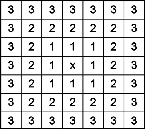We assume that the probability goes up or down in proportion to some function f when we are approaching the coastline from inside or from outside of the ‘spot-lake’. Function f depends on separation only and does not depend on direction. In pixel space, it is easy to estimate the separation from the pixel (i, j) to another pixel according to the ring number (see Fig. 2). Then, we calculate as follows. For pixels belonging to the ‘spot-lake’ L:

Fig. 2.  Numbering of rings around the central pixel (i, j) marked by cross.

and for pixels not belonging to the ‘spot-lake’ L:

Here, n is the number of the ring inside the influence radius (see Fig. 2), m _n is the number of pixels in this ring defined differently than the pixel (i, j) (see above), f (n) is the influence function. We used here , pixels and the quadratic influence function . Note that although the neighbouring ‘spot-lake’ on the map may be defined as the different lake erroneously, this method does not allow for two ‘spot-lakes’ to be correspondent to one lake in reality.

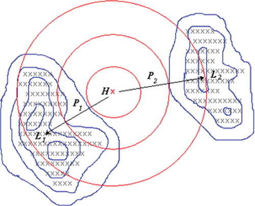
The order of operations in our algorithm is the following (see Fig. 3 for illustration). For every lake H from the dataset for individual lakes, we find on a raster map the pixel (i, j) corresponding to the coordinates of the lake and calculate probabilities P _h in neighbouring pixels within the influence radius R _h . We find all ‘spot-lakes’ in the area around this pixel within the radius (R _h +R _b ). For each of these ‘spot-lakes’ L _i, we calculate the field of probabilities P _b . In every pixel within the radius R _h, we calculate the total probability P of the event that the lake H coincides with the ‘spot-lake’ L _i as the product . Then for every ‘spot-lake’ L _i, we find maximum P in this area and set the correspondence between the ‘spot-lake’ L _i and the lake H, having the probability P. As a result, every ‘spot-lake’ on a raster map L gets several correspondences with H-lakes from the dataset for individual lakes. If L gets more than one correspondences, we choose one with maximum probability, and the ‘spot-lake’ L gains the appropriate mean lake depth from the dataset for individual lakes. If for the ‘spot-lake’ L no correspondences were found, it was not recognised, and it gains the default value of the mean lake depth. For the default, we used 10 m value. The same default depth was used for the recognised lakes but with missing lake depth in the dataset for individual lakes. All pixels classified on the raster map as ‘river’ received the default depth value of 3 m.

Fig. 3.  Modelled field of probabilities for mapping of lakes. Grey crosses represent lake pixels of a raster map. In this example, there are two ‘spot-lakes’ on the raster map, L ₁ and L ₂ . The pixel, corresponding to the coordinates of any point on the surface of lake H from the dataset for individual lakes, is marked by red cross. Lines of equal probabilities P _h and P _b are in red and in blue, respectively (see texts for explanation of symbols). P are total probabilities obtained as maximum from the field of product of P _h and P _b . Lake H then gains the correspondences with ‘spot-lakes’ L ₁ and L ₂ with the probabilities P ₁ and P ₂ , respectively.

Apart from random errors in the lake coastlines, raster maps also contain sea/lake muddling errors. Quite often narrow bays and fjords are erroneously referred to as lake water instead of sea water on a raster map. These errors were corrected automatically by the mapping software, see Kourzeneva (2010) for details. Sometimes, lakes are erroneously referred to as sea water. Errors of this type are more difficult to correct. We correct them only for obvious cases, for the territories that may be considered as ‘land’ according to the rough 2.5 ° resolution land–sea mask. Errors of this type may still occur in the sea coastal zone. Fortunately, these mistakes are not so important for atmospheric models, as extrapolation of the sea surface temperature to these close inland water points will not give unrealistic values.

Currently, only data from the dataset for freshwater lakes are processed, data for saline lakes are not mapped. We applied the mapping method twice. The first run was used to detect and to fix the large errors in the dataset for individual lakes (especially for errors in coordinates of large lakes). After the second run, the final product was obtained.

The bathymetry for large lakes was added in a second step. Firstly, the gridded bathymetry for different lakes with different resolution was linearly interpolated to the ECOCLIMAP2 grid adjusting the coastline by the nearest-neighbour extrapolation method. Then, the mean lake depth values in every pixel were replaced by the bathymetry.

3.4. The dataset

The global gridded lake depth dataset has a resolution of 30 arc sec. (approximately 1 km). It contains basically the mean lake depth, and for several large lakes it provides the bathymetry. Figure 4 gives an example of data for the territory around lakes Vanern and Vattern in Sweden. The additional dataset with coded information about the origin and reliability of data is also provided. The origin code according to Table 1 is given for every pixel. This information is useful for further developments and in estimating the quality of the modelling results.

Fig. 4.  The fragment from the gridded lake depth dataset with 30 arc sec. resolution: the lake depth, m for the territory around lakes Vanern and Vattern in Sweden.

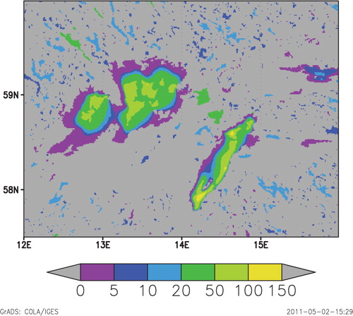
Table 1. Legend for the coded information about the origin of the lake depth data

0	No inland water.
1	The lake was not recognised; the default lake depth value was used.
2	The lake was recognised but with the missing lake depth information in the dataset for individual lakes; the default lake depth value was used.
3	The lake was recognised, the real depth value was used.
4	A river, the default depth value for rivers was used.

4. Projection onto an atmospheric model grid and consistency of data on different grids

4.1. Interpolation of data

Different atmospheric models use different grids, and interpolation from one grid to another is done quite commonly. Gridded representation of the lake data gives an illusion that it is possible to treat lake properties in the same way as atmospheric fields, which is certainly wrong. This mistake can appear when projecting the lake-related information onto an atmospheric model grid. The field of lake depth is discontinuous; thus, interpolation between different grids is incorrect in principle. An interpolation of the mean lake depth between two separate lakes is basically not justified. A small, deep lake and a large, shallow lake are not equivalent to a large lake with a medium depth. But, aggregation is correct if we make a histogram (empirical probability density function). Usually, the atmospheric model grid is coarser than the lake depth dataset grid (30 arc sec.). This makes possible to aggregate the high resolution data using mode statistics, or the most probable lake depth value in every grid box of an atmospheric model grid. The aggregating method was discussed in Kourzeneva (2010). We recommend applying this method for the gridded lake depth field presented here. The grids used by atmospheric models have extremely various characteristics. As an example, the regional models COSMO (Steppeler et al., 2003) and HIRLAM (Undén et al., 2002) are based on a rotated longitude–latitude grid, and the global models GME (Majewski et al., 2002) and ICON (Gassmann and Herzog, 2008; Rípodas et al., 2009; Gassmann, 2010) are based on an icosahedral grid. In order not to transfer very fine resolution lake depth data to the coordinate system of an atmospheric model, we proposed to approximate an atmospheric model grid box by a polygon in geographical (longitude and latitude) coordinates, and then to use a polygon test, e.g. with a crossing number algorithm (Hormann and Agathos, 2001), to specify if the pixel of the fine grid belongs to the grid box in question of an atmospheric model grid. Then, we use lake depth data on the fine grid within the grid box of the atmospheric model grid to calculate statistics. From fine resolution data, a depth histogram may be obtained for every grid box of an atmospheric model grid, with gradations in depth on x-axis and the percentage of lake pixels in certain depth gradation on y-axis. From the histogram, we obtain mode statistics, or the depth value corresponding to the gradation with maximum percentage. This is the most probable lake depth for this grid box in question, and it is the representative of the lake depth value parameter for the parameterisation of lakes in an atmospheric model. We may use an average lake depth value instead, although it is not correct if the distribution is far from Gaussian. From the histogram, one also could easily calculate the total percentage of lakes in the atmospheric model grid box by summarising the percentage numbers in all gradations. The same procedure with making a histogram may be applied for the origin of information code field as well (see Table 1). The most probable information code number in the atmospheric model grid box is useful when estimating the quality of model parameters and the reliability of modelling results. As an example, fields of the lake fraction and the mean lake depth for the atmospheric model grid are displayed in Fig. 5. The grid with the resolution of 0.1 ° is specified in rotated spherical coordinates with new South Pole located in the point with geographical coordinates of 30 °E in longitude and of 30 °S in latitude.

Fig. 5.  (a) Lake fraction, 0–1, and (b) the mean lake depth, m for the atmospheric model grid with 0.1 ° resolution in rotated spherical coordinates, the coordinates of rotated South Pole are (30 °, −30 °). The domain covers the area around Baltic Sea and includes Lake Ladoga, Lake Onega, Lake Vanern, Lake Vattern, Rybinskoe Reservoir and Lake Peipsi.

4.2. Consistency check

The consistency of land cover maps used in an atmospheric model needs to be checked. A mismatch between the main land cover map, used by the atmospheric model and ECOCLIMAP2, used for mapping of lakes, may draw conflicts. Conflicts reveal when the external parameters are aggregated to the atmospheric model (target) grid. A necessary condition for the consistency is that the sum of the fractions of all surface types should be equal to 1:

FR_LAND+FR_LAKE+FR_OCEAN=1.0,

where FR_LAND is the area fraction of a model grid element covered by land, FR_LAKE and FR_OCEAN are the area fractions of a model grid element covered by lake water and by ocean (sea) water, respectively. This condition is not always fulfilled because fractions may be calculated from different maps. Adjusting fractions is not so trivial because we must choose the decisive map a priori, but we do not know what map is really better. The problem is even more complicated if the main land cover map of an atmospheric model does not distinguish between lake water and ocean water. The very noticeable case for this is GLC2000, which is very popular in atmospheric modelling. If one of our maps does not distinguish between lake water and ocean water, it seems natural to choose the map distinguishing between them as a reference. But then, isolated ocean grid elements might erroneously occur within the continents. The best option is to update the main map to make it recognise inland water bodies, although this may not be simple. A default value of 10 m can be assigned for grid elements that have not been assigned a valid lake depth from the database.

5. Discussion

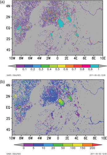
The quality of the final product is highly dependent on the presence of data in the dataset for individual lakes. The illustration is given by Fig. 6 with the code of the origin of information (Table 1) for three regions rich and poor in data. For Poland, comprehensive information for individual lakes is available, and here almost all lakes are recognised and attributed a lake depth. For Karelia, less information are available, thus only several large lakes are recognised and get the mean lake depth. For Alaska, the information is very scarce and even large lakes are not recognised. It is very important to maintain the product in the future, adding new information and correcting data. The structure of the database allows for easy additions of new lake data and error corrections. In principle, it is also not technically difficult to change the raster map if necessary.

Fig. 6.  The gridded code number of the origin of information (see Table 1 for a legend) for (a) Poland, (b) Karelia (c) Alaska.

Some indirect estimations of the mean lake depth are needed in addition to measured data. In some regions (e.g. Northern Canada, Siberia) for many thousands of small lakes, the depth is not instrumentally measured. It could be estimated from the geographical location and the geological origin of lakes (Kitaev, 1984; Doganovsky, 2006; Kondratiev, 2010). According to Kondratiev (2010), the majority of lakes in Southern Finland have the mean lake depth of 2.5–5 m, but for the Caucasus region the distribution of the lake depth has no pronounced maximum and it is impossible to predict the mean depth of lakes. In the boreal zone, estimations of the mean lake depth can be done for the lakes of glacial origin and for thermokarst lakes.

All examined land cover datasets still contain large errors, and some manual work is needed to fix them. In our study, 10 lakes with a surface area of more than 100 km² are found to exist in the dataset for individual lakes but they are not in any of the four examined raster maps. Among the ‘non-existing’ lakes, there is Lake Toshka in Egypt with a surface area of 1300 km². An improvement and inter-comparison of the different maps are still needed. By now, only a rapid inter-comparison of different land cover datasets has been done. An efficient methodology to evaluate different raster maps with respect to water coverage must be developed. Raster maps with better resolution, such as GlobCover (with resolution of 300 m), may be helpful, keeping in mind that they also have random errors.

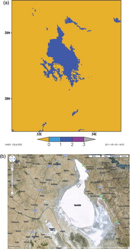
The handling of saline lakes is still an open question. They have very specific characteristics, in particular a time-varying surface. Some of them are very large, and even a 1 km grid map may be completely wrong. For instance, Lake Tuz in Turkey has a surface varying between 1600 and 2500 km², a mean lake depth of 5 m and a salinity of 340‰. Figure 7 shows the ECOCLIMAP2 representation of this lake and what can be seen from remote sensing.

Fig. 7.  Lake Tuz in Turkey, (a) as represented by ECOCLIMAP2, and (b) from remote sensing image. Dark blue colour is lake water, yellow is land.

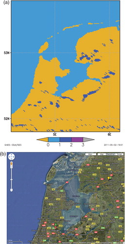
A good distinction between different types of inland water bodies is also still problematic. As mentioned by Lehner and Döll (2004) and Merchant and MacCallum (2009), sometimes the definition what is a lake in reality is rather questionable. It is difficult to distinguish between rivers and lakes in some areas. Rivers are defined in our raster maps very poorly as they are represented as chains of lakes. The GLWD map is of slightly better quality than other maps, but improvements are needed (Lehner and Döll, 2004). Figure 8 shows an example for the middle Amazon River from ECOCLIMAP2 (a) and from GLWD (b). It is also very difficult to distinguish between river estuary water and sea water. These fuzzy areas may be quite large. The illustration is given by Fig. 9 with the estuary of the Amazon River represented by ECOCLIMAP2. Coastal lagoons, even freshwater ones, are very often treated by land cover datasets as ‘sea water’. For example, Lake Ijsselmeer (surface area is 1100 km², mean lake depth is 2 m) and Lake Markermeer (surface area is 700 km², mean lake depth is 5 m) in the Netherlands are treated by ECOCLIMAP2 as sea water (see Fig. 10). In principle, the modelling error may not be significant when using the sea surface temperature for these water bodies instead of the lake surface temperate. But technically, it is not possible to apply the lake parameterisation for them.

Fig. 8.  Middle of the Amazon River as represented by ECOCLIMAP2 (a) and GLWD (b). Dark blue colour is lake water, magenta is river water and yellow is land.

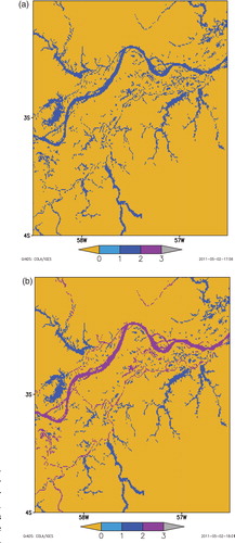
Fig. 9.  The estuary of the Amazon River as represented by ECOCLIMAP2. Dark blue colour is lake water, blue is sea water and yellow is land.

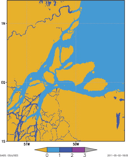
Fig. 10.  Lake Ijsselmeer and Lake Markermeer in the Netherlands as represented by ECOCLIMAP2 (a) and from the remote sensing image (b). Dark blue colour is lake water, blue is sea water and yellow is land.

More bathymetry information for large lakes should be added in future versions of the dataset. Bathymetry maps for many large lakes in digital or in graphic form do exist. The main problem is to make them available and if necessary to digitise them. Currently, the list of lakes with a surface area more than 200 km² and with a lack of bathymetry includes 420 lakes. In addition, it is also advisable to add the bathymetry for the lakes excluded in the present work (very deep lakes, shallow lakes and U-shaped bottom lakes). Even if in these cases the sensitivity of surface temperature patterns to variations in bathymetry is quite low, other important effects coming from the bathymetry may appear. Note that the accuracy of the bathymetry in our dataset is suitable only for atmospheric modelling and some hydrological or environmental applications, but not for navigation.

6. Conclusion

This study presented version 1 of a new global gridded dataset of lake coverage and lake depth specially designed for NWP and climate models. The dataset contains the mean lake depth or the bathymetry in geographical coordinates with the resolution of 30 arc sec. An additional dataset with the coded information about the origin of data is provided. Gridded information is obtained by mapping data from the dataset for individual lakes comprising ca. 13 000 lakes onto the ECOCLIMAP2 land cover map.

This dataset improved the prototype described in Kourzeneva (2010). A specific mapping method, which considered random errors in the dataset for individual lakes and in the coastline of the raster map, was developed. The method solves the optimisation problem by maximising modelled probabilities to match lake depth data and the lake occurrence in the land-cover map. As this method is fully automatic, it will allow easy updates of the database in the future. To project the gridded lake depth data onto an atmospheric model grid, the aggregation method using histograms (empirical probability density functions) is highly recommended.

Currently, the database is being implemented into different NWP and climate models of several institutions and consortia: models of ECMWF (European Center for Medium-Range Weather Forecasts), COSMO (COnsortium for Small-scale Modelling) model, HIRLAM (High Resolution Limited Area Model), ICON (icosahedral nonhydrostatic global model of Deutscher Wetterdienst and Max Planck Institute, Hamburg), Rossby Center model. It is implemented into the externalised surface scheme SURFEX (Le Moigne et al., 2009) that is used in the MesoNH model (developed jointly with the Laboratoire d'Aérologie, Toulouse), in the NWP models AROME/ALADIN/ARPEGE, in the new prognostic system in Nordic countries HARMONIE, and also for monitoring and research purposes.

In the future, updates of the database are foreseen. Additional data will be entered into the database for individual lakes and improved maps will be produced. In addition, the following must be considered in the future:

• inclusion of indirect estimates of the lake depth depending on geological origin and geographical location,

• fixing large errors in the coastline,

• adding bathymetry data for large lakes,

• development of the improved methodology for assessing the quality of raster maps, and

• improvement of the distinction between lakes, rivers and coastal lagoons.

Updating the database by the indirect estimates of the depth depending on geological origin and geographical location of lakes is already an ongoing research.

All products from this study, the gridded datasets, the datasets for individual freshwater and saline lakes, the metadata as well as the Fortran90 routine aggregating and projecting data onto an atmospheric model grid can be freely downloaded from the lake model FLake web page (http://nwpi.krc.karelia.ru/flake/).

7. Acknowledgements

The authors thank Suleiman Mostamandi and Sergey Kondratiev (Russian State Hydrometeorological University) for the help with digitising the bathymetry, Dmitrii Mironov (Deutscher Wetterdienst), Patrick Samuelsson (Swedish Meteorological and Hydrological Institute) and Patrick Le Moigne (Météo-France) for useful discussions. Special thanks to Vladimir Kurzenev and Alina Barbu for discussions on mathematical aspects of the mapping method. Two anonymous reviewers made many useful remarks. The dataset for individual lakes was made possible by people who kindly provided lake data, their names are listed in the dataset header. The project was supported by COSMO, Deutscher Wetterdienst, by the HIRLAM consortia and by Météo-France.

Notes

¹In fact, it is not correct because with a certain map resolution, some lakes with long narrow straits may break down into several non-conterminal areas.

²Although this assumption is not always true.

³Here we ignore the resolution issue and assume that the pixel belongs to the lake entirely.

References

- Amante, C and Eakins, B. W. 2009. ETOPO1 1 Arc-Minute Global Relief Model: Procedures, Data Sources and Analysis. NOAA Technical Memorandum NESDIS NGDC-24. 3, 1–19. Data available online at http://www.ngdc.noaa.gov/mgg/global/global.html.
- Bertholomeé E. Belward A. S. GLC2000: a new approach to global land cover mapping from Earth observation data. Int. I. Remote Sensing. 2005; 26(9/10): 1959–1977.
- Bicheron, P, Amberg, V, Bourg, L, Petit, D, Miras, B and co-authors. 2006. GLOBCOVER: a 300 m global land cover product for 2005 using ENVISAT/MERIS time series. Proceedings of the Recent Advances in Quantitative Remote Sensing Symposium. Valencia, September 2006.
- CEC., 1993. CORINE Land Cover technical guide. European Union. Directorate-Generale Environment. Nuclear Safety and Civil Protection,: Luxembourg.
- Champeaux J. -L. Han K. -S. Arcos D. Habets F. Masson V. Ecoclimap2: a new approach at global and European scale for ecosystems mapping and associated surface parameters database using SPOT/VEGETATION data – First Results. Int. Geosci. Remote Sens. Symp. 2004; 3: 2046–2049.
- Doganovsky, A. 2006. Spatial patterns of lake depressions. Proceedings of the conference “LIX Herzen readings”, Geography and allied sciences. 15–23. in Russian.
- Eerola K. Rontu L. Kourzeneva E. Shcherbak E. A study on effects of lake temperature and ice cover in HIRLAM. Boreal Env. Res. 2010; 15: 130–142.
- ETOPO5.: Data Announcement 88-MGG-02, Digital relief of the Surface of the Earth. NOAA, National Geophysical Data Center, Boulder, Colorado, 1988. Also available online at http://www.ngdc.noaa.gov/mgg/global/etopo5.html.
- ESRI.: Environmental Systems Research Institute. 1992. ArcWorld 1:3 Mio. Continental Coverage. RedlandsCA. Data obtained on CD.
- ESRI.: Environmental Systems Research Institute. 1993. Digital Chart of the World 1:1 Mio. RedlandsCA. Data obtained on 4 CDs. Also available online at http://www.maproom.psu.edu/dcw/.
- Farr, T. G, Rosen P. A, Caro E, Crippen, R, Duren R and co-authors. 2007. The Shuttle Radar Topography Mission. Rev. Geophys. 45, RG2004, 10.3402/tellusa.v64i0.15640.
- Gassmann, A. 2010. Non-hydrostatic modelling with ICON. Proceedings of the ECMWF Workshop on Nonhydrostatic Modelling. European Centre for Medium-Range Weather Forecasts Available at http://www.ecmwf.int.
- Gassmann A. Herzog H. -J. Towards a consistent numerical compressible non-hydrostatic model using generalized Hamiltonian tools. Quart. J. Roy. Meteor. Soc. 2008; 134: 1597–1613.
- Hormann K. Agathos A. The point in polygon problem for arbitrary polygons. Comput. Geom. Theory Appl. 2001; 20: 131–144.
- ILEC.: International Lake Environmental Committee. 1988–1993. Survey of the State of World Lakes. Data books of the world lake environments. Vols. 1–5. ILEC/UNEP Publications, Otsu, Japan. Also available online at http://wldb.ilec.or.jp/.
- Kitaev, S. 1984. Ecological basis of lakes’ bioproduction in different landscapes. “Nauka”, Moscow, 208. (In Russian).
- Kondratiev, S. 2010. External parameters for the parameterization of lakes in NWP and climate modeling. Diploma Thesis, monography, 51. (In Russian).
- Kourzeneva, E. 2009. Global dataset for the parameterization of lakes in Numerical Weather Prediction and Climate modeling. ALADIN Newsletter. 37, July–December, F. Bouttier and C. Fischer, Meteo-France, Toulouse, France, 46–53. Available online at: http://www.cnrm.meteo.fr/aladin/IMG/pdf/FULL-3.pdf.
- Kourzeneva E. External data for lake parameterization in Numerical Weather Prediction and climate modeling. Boreal Env. Res. 2010; 15: 165–177.
- Lehner B. Döll P. Development and validation of a global database of lakes, reservoirs and wetlands. J. Hydrol. 2004; 296(1–4): 1–22.
- Le Moigne, P, Boone, A, Calvet, J.-C, Decharme, B, Faroux, S and co-authors. 2009. SURFEX scientific documentation. CNRM-GAME, Météo France: France.
- Loveland, T. R, Reed, B. C, Brown, J. F, Ohlen, D. O, Zhu, J and co-authors. 2000. Development of a global land cover characteristics database and IGBP DISCover from 1-km AVHRR data. Int. I. Remote Sens. 21 (6/7), 1303–1330. Data and documentation available online at: http://edc2.usgs.gov/glcc/glcc.php.
- Majewski, D, Liermann, D, Prohl, P, Ritter, B, Buchhold, M and co-authors. 2002. The Operational Global Icosahedral-Hexagonal Gridpoint Model GME: Description and High-Resolution Tests. Mon. Wea. Rev. 30, 319–338.
- Martynov A. Sushama L. Laprise R. Simulation of temperate freezing lakes by one-dimensional lake models: performance assessment for interactive coupling with regional climate models. Boreal Env. Res. 2010; 15: 143–164.
- Masson V. Clampeaux J. L. Chauvin F. Meriguet C. Lacaze R. A global database of land surface parameters at 1-km resolution in meteorlogical and climate models. J. Climate. 2003; 16: 1261–1282.
- Merchant, C. J and MacCallum, S. N. 2009. ARCLake Quaterly Report no. 1. The University of Edinburg, 3. Data available at: http://www.geos.ed.ac.uk/arclake.
- Mironov, D. 2008. Parameterization of lakes in numerical weather prediction. Description of a lake model. COSMO Technical Report. vol. 11. Deutscher Wetterdienst, Offenbach am Main, Germany, 41.
- Rípodas, P, Gassmann, A, Förstner, J, Majewski, D, Giorgetta, M and co-authors. 2009. Icosahedral Shallow Water Model (ICOSWM): results of shallow water test cases and sensitivity to model parameters. Geo. Model Develop. 2, 231–251.
- Samuelsson P. Kourzeneva E. Mironov D. The impact of lakes on the European climate as simulated by a regional climate model. Boreal Env. Res. 2010; 15: 113–129.
- Steppeler, J, Doms, G, Schättler, U, Bitzer, H. W, Gassmann, A and co-authors. 2003. Meso-gamma scale forecasts using the non-hydrostatic model LM. Meteorol. Atmos. Phys. 82, 75–96.
- Tranvik, L. J, Downing, J. A, Cotner, J. B, Loiselle, S. A, Streigl, R. G and co-authors. 2009. Lakes and reservoirs as regulators of carbon cycling and climate. Limnol.Oceanogr. 54 (6, part 2), 2298–2314.
- Undén, P, Rontu, L, Järvinen, H, Lynch, P, Calvo, J and co-authors. 2002. The HIRLAM-5 scientific documentation. SMHI: Sweden.
- Walter K. Smith L. Chapin III F. Methane bubbling from northern lakes: present and future contributions to the global methane budget. Phil. Trans. R. Soc. A. 2007; 365: 1657–1676.