Optimal placement of mobile sensors for data assimilations

ABSTRACT

We explore the theoretical framework as well as the associated algorithms for the problem of optimally placing mobile observation platforms to maximise the improvement of estimation accuracy. The approach in this study is based on the concept of observability, which is a quantitative measure of the information provided by sensor data and user-knowledge. To find the optimal sensor locations, the observability is maximised using a gradient projection method. The Burgers equation is used to verify this approach. To prove the optimality of the sensor locations, Monte Carlo experimentations are carried out using standard 4D-Var algorithms based on two sets of data, one from equally spaced sensors and the other from the optimal sensor locations. The results show that, relative to equally spaced sensors, the 4D-Var data assimilation achieves significantly improved estimation accuracy if the sensors are placed at the optimal locations. A robustness study is also carried out in which the error covariance matrix is varied by 50% and the sensor noise covariance is varied by 100%. In addition, both Gaussian and uniform probability distributions are used for the sensor noise and initial estimation errors. In all cases, the optimal sensor locations result in significantly improved estimation accuracy.

• sensor placement
• observability
• optimisation
• data assimilation
• 4D-Var

1. Introduction

One of the important components of the numerical weather prediction (NWP) is atmospheric data assimilation. Atmospheric data assimilation provides the best available state estimate (i.e. the initial conditions) to be used in NWP. It is a procedure to combine all the available prior information, such as background, prediction model, observations, observation operators, and the associated error statistics, to obtain the state estimate using proper mathematical techniques. In the same community of data assimilation, various techniques, such as variational algorithms (e.g. 3D-Var and 4D-Var) and ensemble Kalman filters (e.g. EnKF) as well as hybrid variational/ensemble algorithms, are currently used in atmospheric data assimilation.

It is well known within the data assimilation community that not every observation has the same impact on the NWP forecast. The observation impact depends on the information content of each assimilated observation and the data assimilation system used to assimilate it. It is highly desirable to know the potential impact of each observation on short term NWP forecasts or some other measures of interests. Virtually all the existing researches in this area are based on the pioneering work of Baker and Daley (2000). They introduced the concept of observation sensitivity (also known as the gradient of atmospheric analysis with respect to the observations). Baker and Daley (2000) showed that observation sensitivity is simply the adjoint of the data assimilation system. They also provided an elegant way to construct the adjoint of an observation-space variational data assimilation system. Langland and Baker (2004) proposed a technique to routinely calculate the observation impact on short term NWP forecasts (24 hr forecast in their case). The technique requires: a) the adjoint of the US Navy's global NWP model (NOGAPS, see Hogan and Rosmond (1991); Rosmond (1997)) to provide the sensitivity of the 24 hr forecast errors with respect to the initial condition; b) the adjoint of the US Navy's 4D-Var data assimilation system [NAVDAS-AS, see Xu et al. (2005)]. Their results provided very useful inside information that was impossible to obtain before.

Because observations play such an important role in the data assimilation and in the subsequent forecast, many additional studies to address various aspects of the observation impact have been conducted since 2000 at various institutions around the world. The following is a list of works related to the variational data assimilation algorithms: Cardinali et al. (2004); Xu et al. (2006); Daescu (2008); Tremolet (2008); Baker and Langland (2009); Cardinali (2009); Daescu and Todling (2009, 2010); Gelaro and Zhu (2009); Gelaro et al. (2010); Cardinali and Prates (2011). Similar studies were also conducted for ensemble data assimilation methods, such as Liu and Kalnay (2008), Liu et al. (2009), and Li et al. (2009). Despite the success in the area of observation impact, this can only provide the observation impact information after the observation is already assimilated and the analysis is used as the initial condition to make the short term forecast. Currently it is not possible to deal with the issue of optimal sensor placement in the planning of the targeting observation during a field experiment.

In this study, we explore the theoretical framework as well as the associated algorithms for the problem of optimally placing mobile observation platforms to maximise the improvement of estimation accuracy. The current adjoint (or ensemble) based observation monitor system can provide the evaluation of the observation impact only after the fact. A comprehensive solution to the planning of optimal sensor placement is still an open problem. In our approach, the optimal sensor locations are calculated around a nominal trajectory or a forecast defined by an initial state u ₀. This is necessary because, for non-linear systems, the observability is trajectory dependent. Using the same sensor locations, the observability can have significant change around different trajectories. For sensors with mobility, the issue of unknown nominal trajectory is resolved using a moving horizon approach. The optimal sensor locations are found based on the current approximate of the system trajectory. After a period of time, an updated estimate of the system trajectory is computed and a forecast is given. Based on that, a new set of optimal sensor locations are found and the sensors are relocated. The process is repeated in a time interval synchronised with the estimation and forecast process.

The theory and algorithm developed in this study are based on the concept of observability, which is a quantitative measure of the information provided by sensor data and user-knowledge. The observability can be numerically computed based on the system's dynamic model. It provides the cost function for the optimisation of sensor locations. In this study, the Burgers equation is used to verify the theory and the approach. In the computation, the system's observability is numerically approximated using an empirical Gramian matrix method (to be explained below). Then the observability is maximised using a gradient projection method to find the optimal sensor locations. To verify the optimality of the method, Monte Carlo numerical experiments are carried out using standard 4D-Var algorithms based on two sets of data, one from equally spaced sensors and the other from the optimal sensor locations. The results show that, relative to equally spaced sensors, the 4D-Var data assimilation achieves significantly improved estimation accuracy if the sensors are placed at the optimal locations. A robustness study is also carried out in which the initial error covariance matrix is varied by 50% and the sensor noise covariance is varied by 100%. To further test the robustness, the numerical experiments are implemented using various sets of data with both Gaussian and uniform probability distributions. In all cases, the optimal sensor locations result in significantly improved estimation accuracy.

The study is organised as follows. In Section 2, the concept of observability is introduced for general dynamical systems. Its approximation using an empirical Gramian matrix is also introduced. In Section 3, the problem of optimal sensor placement is formulated and a gradient projection method is introduced for its computation. In Section 4, the concept and the algorithms are applied to a system defined by the Burgers equation as an illustrative example. The optimal sensor locations are found. In Section 5, a standard 4D-Var data assimilation method is applied to test the optimal sensor locations. In Section 6, the robustness of the optimal sensor locations is tested using several covariance matrices as well as different probability distributions. At the end of this section, we revisit the definition of observability to address some related issues on the norms and metrics used in the concept.

2. Observability

The concept of observability has been widely used in control system theory and its applications. In this study, we follow the recent research work by Kang and Xu (2009a, 2009b) on the quantitative measure of observability. Consider a discrete-time dynamical system1

where is the state variable of the system, k is an integer representing the time steps since the initial time, and f is a function of (k,u). If the original model is defined by a continuous-time differential equation, then (1) represents its discretisation where u(k) is the state of the system at grid points. Let λ be a parameter that defines the sensor configuration. In this study, λ represents the locations of the sensors in space. However, the concept is applicable to other sensor parameters such as path, orientation, and density. The output, denoted by y(k), of eq. (1) is the variable measured by sensors. It is a function of the state variable and sensor locations,

In the simulations, h(u,λ) is computed using spline if λ is not located at grid points. Other interpolating algorithms are applicable as well. To summarise, we study the observability of the state variable based on the following system model:2

Let u(k;u ₀ ), k=0,1, …, N _t , be the trajectory of the system with initial state u(0;u ₀)=u ₀. The corresponding output is denoted by y(k,λ;u ₀), i.e.

In the following, we define the observability of u(0). The definition can be generalised to the observability of the state at any time, k=k ₀. Consider a nominal trajectory u(k;u ₀), k=0,1, …, N _t . The variation of the measured variable y(k) under the variation of u ₀ is defined as follows:3

where P ₁ is a weight matrix that reflects our confidence on the background from the previous estimation process step or the initial guess. If P ₁ is large, the background is most likely close to the true value, which implies a good observability. Similar to data assimilation, P ₁ can be assigned as the inverse matrix of the background error covariance. In this study, the term including P ₁ is not applied so that the study is focused on the second term in eq. (3), which represents the impact of the sensor information. We adopt the following norm for .

where . Because y(·) represents the output from various types of sensors with different error probability distributions, P ₂ in eq. (3) is a weight matrix, for instance, the inverse matrix of the sensor noise covariance. In addition, P ₂ can be used to weight the importance of different sensors in a data assimilation process, which is a potential application of the concept to sensor assessment.

The state space of the system is . However, it is not necessarily the space used for the estimate, or the space of estimation. For large scale systems with high dimension N _u , it is often the case that a low dimensional subspace is able to provide adequate estimation accuracy. For the definition of observability, we introduce the space for estimation, . The space has a norm, , which is the same norm that we use to measure the error of an estimated u ₀. We assume that the estimate is updated at each time step using vectors in W. The following definition of observability is the discrete-time version of a special case defined in Kang and Xu (2009a). It agrees in spirit with the approach in Krener and Ide (2009).

Definition 1. Let ρ>0 be a positive number. Then the number ɛ is defined as follows4

The ratio ρ/ɛ is a measure of observability. It is called an unobservability index.

The value of ɛ represents the smallest variation of y corresponding to variations of u ₀. A small value of ɛ implies that u ₀ is less observable. In the extreme case of ɛ=0, it implies that the sensor cannot detect the variation of u ₀ in at least one direction; and P ₁ does not contain any information about the accuracy of the initial guess in the same direction. Therefore, u ₀ is unobservable. The value of δu ₀ obtained from solving the optimisation problem [eq. (4)] represents the direction of δu ₀ in which the sensors and initial guess are least sensitive or accurate. To summarise, a small value of ρ/ɛ implies strong observability. For the case of linear systems with , the ratio ρ/ɛ equals the value of unobservability index defined in Krener and Ide (2009). If we consider J in eq. (3) as the error of sensors and ||δu ₀|| as the estimation error, then ρ/ɛ=1 implies that the magnitude of the worst error in the estimation of u ₀ is at about the same level as the sensor error. If ρ/ɛ belongs to the interval [1,10] then the worst estimation error is larger than the sensor error, but in the same order of magnitude. Depending on the error tolerance required by data assimilation, for specific systems one can define the ranges of the value of ρ/ɛ in which the system is strongly observable, reasonably observable, weakly observable, and unobservable.

Interested readers are referred to Kang and Xu (2009b) for illustrative examples of observability. The following is an artificial and simple example of an unobservable system. In this case, the unobservability index is ∞. Suppose5

Suppose the sensors are able to measure the value of u ₂, i.e.

Given any initial condition u ₀=[u ₀₁ u ₀₂ u ₀₃] ^T , we can generate two trajectories using u(0)=u ₀ and u(0)=u ₀+[0.1 0 0] ^T , i.e. ρ=||δu ₀||=0.1. It is obvious that the two different trajectories of u(k) result in the same value of y(k). In other words, the sensor completely fails to catch the change of value in the initial condition. In this case, ɛ=0 because the cost in eq. (3) equals zero, where we assume P ₁=0 (no a priori statistical information about the initial condition). Obviously u ₁(0) is not observable. The unobservability index, ρ/ɛ, equals infinity because ɛ=0 .

The system becomes observable if we can measure u ₁(k), i.e.

The system [eq. (5)] with this output can be written into the following matrix form6

If u(k) is a trajectory of eq. (6) with an initial state u ₀, then the trajectory with an initial variation δu ₀ is

Therefore

If we use the Euclidean norm in eq. (3), then

where N+1 is the total number of the sampling data used in the estimation process, and

Therefore, ɛ in eq. (4) satisfies

where σ ² is the smallest eigenvalue of G. Suppose ‖δu ₀‖₂=ρ, then

Following this example, we can approximate the unobservability index for non-linear systems with a small value of ρ. The matrix G can be numerically approximated by a method of empirical Gramian matrix, which is a generalisation of the algorithm in Krener and Ide (2009). Consider the mapping7

From eq. (3), the cost function J(u ₀, δu ₀,λ) is, in fact, the norm of the image of this mapping. The minimisation in eq. (4) is to find the image of the mapping [eq. (7)] with smallest norm subject to ‖δu ₀‖=ρ. Let v ₁,v ₂, … , v _s be an orthonormal basis of the space W. Then the variation of δu ₀ on the sphere can be represented by

where

For each direction v _i , the variation of the output can be estimated empirically by8

for k=0, …, N _t . The mapping [eq. (7)] can be locally approximated by9

Therefore, the minimum value in eq. (4) approximately equals the smallest norm of the images under the mapping [eq. (9)] subject to . More specifically,10

where

Let σ² be the smallest eigenvalue of G, then the smallest norm of the images under eq. (9) subject to is σρ. Therefore, the unobservability index ρ/ɛ is approximated by 1/σ .

In linear algebra, G is called a Gramian matrix. Because we are trying to compute the observability before sensors collecting data and because of the random sensor error, there are endless possible estimates of a state variable. The Gramian matrix G approximates the mapping from the possible estimation error to the variation of the output, or the possible sensor error.

What eq. (4) measures is, in fact, the observability of the initial state u ₀. However, an accurate initial state does not automatically guarantee good accuracy along the entire trajectory. One may want to measure the observability using u(N _t ) , the final state, or other time point u(k), to define the observability. Because a trajectory is uniquely determined by any given u(k) for a fixed time k, it is straightforward to generalise Definition 1 to the observability of any u(k). The selection of k depends on the system or the accuracy requirement of specific applications. To guarantee an overall accuracy, it is also possible to use different norms, such as L ²-norm. This issue is addressed in Section 6.

3. Optimal sensor placement

The concept of observability provides a quantitative measure of the quality of sensor information for the purpose of state estimation. More specifically, the value of ɛ defined in eq. (4) depends on λ, the sensor locations. We treat ɛ as a function of λ, ɛ(λ), which is used as the performance measure of sensor locations. The best sensor locations are those that maximise the value of this performance measure, i.e.11

From Section 2, the value of ɛ(λ) can be computed using the method of empirical Gramian matrix. Therefore, eq. (11) is, in fact, a problem of maximisation with both linear and non-linear constraints. This problem is numerically challenging. Further research is required to find efficient computational methods. For the purpose of proving the concepts of observability and sensor placement, in the following we adopt a projection gradient method to numerically solve eq. (11).

The gradient with respect to λ is defined by

Suppose the location of the ith sensor is bounded by . To find the searching direction on the boundary of the region, the following projected gradient is used.

where is the ith component of . The projected gradient direction guarantees that the searching direction points toward the inside of the boxed region. Thus eq. (11) can be treated as a problem of unconstrained maximisation. Given a search direction , a process of line search is then carried out using the Armijo algorithm model. Details about this line search algorithm are referred to Polak (1997).

4. An example of Burgers’ equation

To verify the concept, the theory is applied to the following Burgers’ equation12

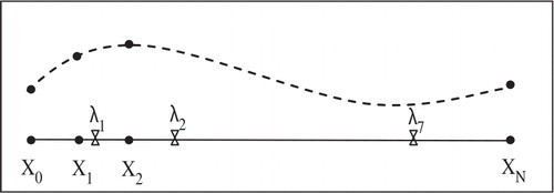
Suppose we can measure the value of U(x,t) at N _y fixed locations in the time interval [0,T]. The question is: what sensor locations maximise the observability around the nominal trajectory U(x,t) ?

For the purpose of computation, we discretise the problem at a set of uniformly spaced nodes,

where

Sensors are located in the interval [0,L], not necessarily at the nodes (Fig. 1). Define u _i (t)=U(x _i ,t) for i=1, 2, … N–1. System [eq. (12)] is discretised using the central difference method13

Fig. 1.  Illustrative graph of nodes in discretisation and sensor locations.

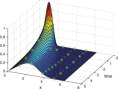
Using the framework in Section 2, the discretised version of eq. (13) represents the dynamical system [eq. (2)]. In all computations that follow, we apply a Runge-Kutta algorithm to eq. (13). The observability is computed around a nominal trajectory defined by the initial value14

In the following, we use eq. (13) as the true model. The locations of the N _y sensors are represented by the parameter

where λ _i is the x-coordinate of the sensor in space. A solution of the system in the (t,x,u)-space with the points of sensor sampling is shown in Fig. 2.

Fig. 2.  A trajectory with sensor locations.

We assume that sensors can be located anywhere in the interval [0,L], not necessarily at the nodes. Because of that, the value of the true solution at the sensor locations is not directly available from the discretised model. For the purpose of computation, the value of sensor data is generated by the following interpolation15

where In(α,β,γ) represents the interpolation of (α,β) evaluated at γ. Because λ is a vector, . In this study, the interpolations are computed using cubic splines. In the framework introduced in Section 2, the output, y, of the system in eq. (2) is defined by eq. (15).

Suppose each sensor collects N _t readings at the frequency in the time interval [0,T], i.e. . The cost function defined in eq. (3) with constant weights has the following expression16

where , t _k =t _k-1+Δt. In this example, the cost does not include the norm of the initial error, i.e. we focus on the observability with respect to the sensor data only. The minimisation in eq. (4) has the following form

The observability is measured by the ratio ρ/ɛ. The smaller is this ratio, the stronger is the observability.

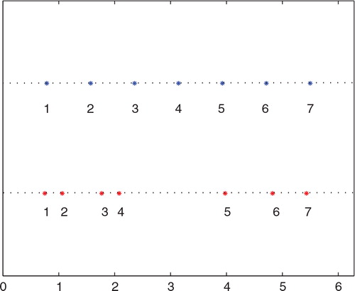
The computations are based on a set of specific parameter values. The number of sensors is seven, i.e. N _y =7. The nodes for discretisation divide the space, [0,2π], into N=50 equal length subintervals. However, the dimension of the space for estimation, W, is much smaller. In fact, we assume that the initial state U(x,0) can be accurately approximated using finite terms of Fourier series,17

The space for estimation, i.e. W in Definition 1, is defined to be all functions in the form of eq. (17). The observability is defined around a nominal trajectory. In this example, the nominal trajectory is defined by the initial state, U ₀(x), which is given below. The plot of the nominal trajectory is shown in Fig. 2. We assume that U(x,t) can be approximated by Fourier series. Therefore, the space for estimation is

where The initial value of the truth is

Details on the parameters used in this example are listed as follows.

Following the formulation and algorithm in Section 3, the optimal sensor locations are computed under the constraints ,18

In this case, the unobservability index is

This number implies that, in the worst case, the error of the u(0) estimate is about 1.75 times the sensor error as measured by the norm J(δu ₀,λ). In other words, a reasonable estimate of u(0) should have an error within 1.75 times the sensor error. Because of different scales used for the state space and sensor errors, the value of unobservability index must be combined with the expected, or standard deviation, of the sensor error to assess the accuracy of state estimate. If the sensor error is at the same scale as the desired bound of estimation error, then ρ/ɛ=1.75 implies that u(0) is observable. On the other hand, independent of the scales of the variables, the unobservability index is directly comparable to other sensor locations. For the purpose of comparison, let us consider the equally spaced sensor locations,19

In this case, the unobservability index is

It is larger than that from optimal sensor locations by more than seven times. We can conclude that the state variable is weakly observable using equally spaced sensors. Its data is much less valuable than those from optimal sensor locations. Therefore we expect significantly larger error in state estimation if sensors are equally spaced, no matter what estimation method is used.

The equally spaced and the optimal sensor locations are shown in Fig. 3. The optimal sensor locations agree with our intuitive sense. It is not the full values of the model state trajectory U(x,t) that are important for the observability, but rather the dynamics of the trajectory. As shown in Fig. 2, U(x,t) is much more dynamically active with relatively high rate of change on the left side in the space. On the right side, U(x,t) is relatively calm. Optimising the observability automatically takes this phenomenon into consideration. As a result, the optimal solution places four sensors on the left side; and leaves three sensors on the right side. Because the observability is relative to nominal trajectories based on forecast, it is desirable that at least some sensors have mobility so that the optimal sensor locations can be updated in real-time and the sensor system is adaptive to the dynamic reality.

Fig. 3.  Sensor locations: equally spaced (blue) and optimal locations (red).

5. Optimal sensor locations for data assimilation

High observability of a trajectory implies that a reasonable estimation method should be able to recover the trajectory with small error. More specifically, if the estimation method is based on the minimisation of the cost function J in eq. (3), then the optimal sensor locations guarantee to minimise the worst error. Data assimilation is based on the minimisation of a cost function. We expect that the concept of observability is applicable to data assimilations. More specifically, we want to verify the following belief: improved observability results in smaller estimation error. For this purpose, data assimilation results using optimal sensor locations are compared to the results from equally spaced sensors. The comparison is based on a set of Monte Carlo experiments using 200 data sets consisting of randomly generated initial background errors and sensor noise.

For each set of data, a standard algorithm of 4D-Var is applied to estimate the trajectory. For the reasons of space, details on the 4D-Var algorithm used in this section are referred to Xu and Daley (2000) and Xu et al. (2007). The tangent linear model and the adjoint model are developed using the algorithm from Rosmond (1997). The linear equations in the data assimilation are solved using a standard conjugate gradient algorithm in Golub and Van Loan (1996).

The data sets for the Monte Carlo experiments are generated randomly. Two hundred sets of background trajectories are generated around the true trajectory with initial state u ₀ in eq. (14). The background, u ^b (t), represents an estimate from the previous step or an initial guess of the true trajectory. The variation of the initial state of backgrounds, u ^b (0) − u ₀, is a random variable with a Gaussian distribution of zero mean. The average of is 0.3638, which is about 11.14% relative to . The data assimilation uses backgrounds that are projected to the space for estimation, W, defined in eq. (4).

In a 4D-Var data assimilation, an estimate u ^a (t) is obtained using the system model as well as sensor information, i.e. the output y(t _i ), which is corrupted by noise. For each background, we generate a set of sensor information with noise20

where y ^true(t _i ) is the value of the true state at the sensor location. The standard deviation of the sensor noise, R, is about 0.7~1% of the average value of u(x,t). Later in the robustness study, it is increased to about 2%. We choose a relatively small noise because this study is specifically focused on the impact on data assimilation by the single factor of sensor locations.

The sensors are not always placed at the grid points of the discretised model [eq. (13)]. Therefore, in the simulations y ^true(t _i ) is not directly available from the model. In the computation of observability, cubic spline is used to approximate its value, which is defined in eq. (15). However, for 4D-Var estimation we adopt a linear interpolation method to approximate y ^true(t _i ) so that the matrix H in the algorithm is easily available. Numerical experiments (results are not shown) confirm that the error caused by the linear interpolation is negligible.

In the Monte Carlo experiments, 200 sets of background are generated as described above,21

The notation in this section is different from previous sections. The sub-index, k, in is not the time step as in previous sections. It represents the index in the Monte Carlo experiments. The time step is represented by t _i . For each background, two sets of sensor data with noise are generated, one based on equally spaced sensors and the other on optimal sensor locations. The sensor data is available only at the sampling point in time and space, i.e. a sequence of the following form22

where N _t =20 and N _y =7. For each combination of background and sensor locations, the analysis, u ^a (t), is found using 4D-Var data assimilation. The analysis is an estimate of the truth. Two norms are used in the evaluation of estimation error from different sensor locations. Let u ^truth(t) be the true trajectory of the system, i.e. the truth. For an analysis, u ^a (t), the overall error of u ^a (t) is measured using the following norm23

where is the norm in . The error of the initial state u ^a (0) is defined by24

Using the backgrounds in eq. (21) and the 4D-Var estimation process, 200 estimate of the truth is numerically generated. The accuracy of the data assimilation is characterised by the root-mean-square error (RMSE) based on the norms eq. (23) and eq. (24),25

for and26

for the initial state, where N is the number of numerical experiments. The RMSE of backgrounds, , is defined in a similar way. In the Monte Carlo experiments, the backgrounds in eq. (21) are randomly generated so that the RMSE of u ^b (·) is 0.3638, which is 11.14% relative to the norm of the truth, u ^truth(t); the RMSE of initial states u ^a (0) equals 0.3524, which is 15.13% relative to the truth u ₀. 4D-Var data assimilations are applied to all backgrounds in eq. (21) with sensor data in the form of eq. (22), from both the equally spaced sensor locations [eq. (19)] and the optimal locations [eq. (18)]. The data assimilation algorithm requires the background error covariance and the sensor noise covariance. They are generated from the set of errors and noise normalised by N _t −1.

The plots of the errors and from the Monte Carlo experiments are shown in Figs. 4 and 5. The estimation accuracy is significantly improved by using the optimal sensor locations. In fact, the RMSE of , k=1,2, …, 200, is 0.0788 for the equally spaced sensor locations. The RMSE is reduced to 0.0325 if the optimal sensor locations are used, which is an improvement of more than 59%. The errors of the initial states have similar behaviour. For equally spaced sensors, the RMSE of initial states is 0.1647; and the value is 0.0786 for optimal sensor locations, which is a 52% error reduction. These results are summarised in Table 1.

Fig. 4.  The scatter plot of ρ/ɛ vs. .

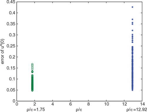
Fig. 5.  The scatter plot of ρ/ɛ vs. ..

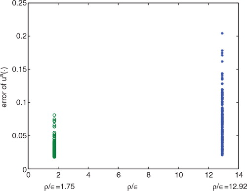
Table 1. Summary of Monte Carlo experiments

	Unobservability index, ρ/ɛ	RMSE of u ^a(0)	RMSE of u ^a(·)
Equally spaced sensors	12.92	0.1647	0.0788
Optimal sensor location	1.75	0.0786	0.0325
Improvement	86%	52%	58%

The Monte Carlo experiments show that the concept of observability is consistent with the outcomes from data assimilation, i.e. data from sensors with higher observability results in higher estimation accuracy. This implies that sensor data with high observability contains more valuable information than those with low observability. However, one might notice from Table 1 that the scale of accuracy improvement does not match with the scale of the observability. In fact, the unobservability index of optimal sensor locations is 1.75 in contrast to 12.92 for equally spaced sensors, i.e. the observability is improved by about 86%. However, the improvement of estimation accuracy is about 50~60% depending on the choice of the norm. This phenomenon is largely due to the error covariance of initial background. In the computation of unobservability index, the impact of the error covariance of is not included in the cost function [eq. (16)]. However, one can certainly take this into consideration as a part of the cost function, i.e. a non-zero P ₁ in eq. (3). In the example of Burgers equation, we ignore the initial error covariance so that the observability is focused on the quality of sensor locations only. On the other hand, if the covariance of the background is known at the time of sensor location design, it can certainly be included in the cost function eq. (3) so that the optimal locations reflect the combined value of the information on both the initial error covariance and the sensor data.

Figure 6 shows the RMSE as a function of time. More specifically, using the 200 analysis resulting from data assimilation we define the following function

Fig. 6.  RMSE as a function of time. Curve: equally spaced sensors. Dash: optimal sensor locations.

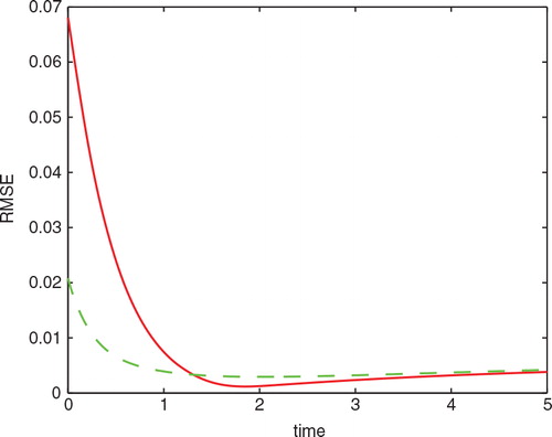
where N=200. In Fig. 6, the curve represents the RMSE from equally spaced sensors and the dash curve represents the result using optimal sensor locations. Due to the non-linear nature of the system, the sensitivity of the state variables to sensor noise is not evenly distributed along a trajectory. Maximising observability results in an overall improvement of the estimation accuracy. More specifically, the optimal sensor locations result in significantly smaller error when the estimation is difficult and relatively inaccurate, which is in the time interval [0,1.3]. To compromise, the optimal sensor locations result in slightly bigger error in [1.3,5] when the estimate is relatively accurate.

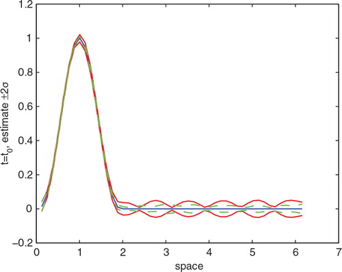
The initial state and the interval of two times standard deviation are shown in Fig. 7, in which the curve is the result of using equally spaced sensors and the dash curve represents the result using optimal sensor locations, which has a significantly smaller error standard deviation.

Fig. 7.  The ±2σ interval around the initial state. Curve: equally spaced sensors. Dash: optimal sensor locations.

6. Robustness analysis and some additional issues

In practical applications, robustness is an important factor in evaluating optimal designs. It is desired that suboptimal or acceptable results can be achieved in the presence of uncertainties. In data assimilations, the specification of the initial error covariance, , is a significant challenge due to its size and uncertainty. In the robustness study, is varied from its true value by about 10%. Then the RMSEs of u ^a (·) using equally spaced sensors and optimal locations are computed, which equal 0.0938 and 0.0351, respectively. If the covariance matrix is changed by about 50% from its true value, the RMSEs become 0.1191 and 0.0887. The results are summarised in Table 2. The robustness is also numerically tested for the sensor noise covariance, R. If the matrix is changed by 100% from the true value, the RMSEs are 0.0646 and 0.0407 for equally spaced sensors and optimal sensor locations, respectively. In all cases, the optimal sensor locations result in significantly improved estimation accuracy, which ranges from 25% to 62% (see Table 2).

Table 2. Summary of a robustness study. The column under % represents the improvement in accuracy by using optimal sensor locations

	Variation of	Variation of R	RMSE of u ^a(·)	%
Equally spaced	10%	0	0.0938
Optimal locations	10%	0	0.0351	62
Equally spaced	50%	0	0.1191
Optimal locations	50%	0	0.0887	25
Equally spaced	0	100%	0.0646
Optimal locations	0	100%	0.0407	37

In addition to the variations of covariance matrices, another study is carried out to test the robustness under different probability distributions. In the previous numerical experiments, the background and sensor noise are both generated using normal distributions. To test the robustness, we generate a set of 200 backgrounds using uniform distribution in the interval of [−0.17, 0.17]. The sensor noise follows uniform distribution in [−0.003, 0.003]. Then 4D-Var data assimilation is applied to this set of data to generate two hundred . The results are shown in Table 3. Consistent to the previous numerical results, the estimation error of u(0) is improved by 35% by using the optimal sensor locations. The improvement in the estimation of u(·) is more than 42%.

Table 3. Summary of Monte Carlo experiments using uniform distributions

	Observability, ρ/ɛ	RMSE of u ^a(0)	RMSE of u ^a(·)
Equally spaced sensors	12.92	0.1376	0.0645
Optimal sensor location	1.75	0.0893	0.0372
Improvement	86%	35%	42%

In the following, we revisit Definition 1 to address some related issues. What eq. (4) measures is, in fact, the observability of the initial state u ₀. More specifically, the meaning of ɛ and ρ can be explained as follows: if the sensor error is bounded by ɛ, then the worst least square estimate u ^a (0) of the initial state u ₀ has an error that is less than or equal to ρ. Because the trajectory of a system is uniquely determined by its initial state, for many systems an accurate estimate of u ₀ results in an accurate estimate of the entire trajectory. However, the initial state is not always the first priority in estimation. For instance, filtering problems require an accurate estimation of the current state, rather than the initial state. In the example of Burgers’ equation, the system is stable in which the trajectory has active non-linear behaviour around the initial time. As a result, we focus on the observability of the initial state. Nevertheless, an accurate initial state does not automatically guarantee a good accuracy along the entire trajectory. In order to accommodate various requirements in estimation and prediction, it is necessary to define observability using different types of norms.

It is straightforward to generalise Definition 1 to the observability of u(k ₀) for any fixed time k ₀. Given any u(k ₀) =u ₀, it uniquely determines a trajectory u(k;u ₀). The associated cost, J(u ₀,δu ₀,λ), can be defined in a similar way as in eq. (3). Let ρ>0 be a positive number. Then the number ɛ is defined as follows27

The ratio ρ/ɛ is a measure of the observability of u(k ₀). This number can be approximated using empirical Gramian matrix method introduced in Section 2, except that eq. (8) is defined using perturbations around u(k ₀).

Instead of focusing on a fixed point in the time interval, observability can be defined for an entire trajectory u(·). For this purpose, the norm of δu must measure the overall error along the trajectory, for instance the l ^p -norm

Given a nominal trajectory u(k), the space W is a subset of differentiable functions such that

u(k)+δ(k) is a trajectory that satisfies the dynamics model [eq. (1)]. For non-linear systems, W is not a linear space. It is a differential manifold with a metric. Although the space of differentiable functions is infinitely dimensional, the tangent space of W has a finite dimension. This is because trajectories are uniquely determined by initial states, which are from a finite dimensional space. Suppose the output, i.e. the sensor measurement, is represented by

The sensor measurement around the nominal trajectory is denoted by y(k;u+δu), i.e.

the variation of the measured variable y(k) around a nominal trajectory is defined as follows28 The observability of u(·) is defined as follows,29

For this definition of observability, the empirical Gramian method can be modified to approximate ρ/ɛ.

7. Conclusions

To summarise, the concept of observability is defined as the theoretical foundation for the optimal design of sensor locations. The method of empirical Gramian matrix is a practical way to approximate the observability. It provides a cost function for the optimisation of sensor locations, which is carried out numerically using a gradient projection method. As a testbed, the Burgers equation is employed in the examples. The concept and computational methods are found applicable to these examples. The results prove that optimal sensor placement leads to significantly improved estimation accuracy in data assimilations when 4D-Var is used; and the performance is tested to be robust.

This work raises many questions for long term research. Optimal trajectory planning is an active research area in control systems in which the path, the control, and the trajectory of unmanned vehicles are designed to optimise a given performance measure (see, for instance, Tang et al. (2011) and references therein). The combination of algorithms in trajectory planning with the concept of observability is an obvious next step of research. The goal is to extend the results in this study on fixed sensor locations to mobile sensors in more dynamic environments. It requires optimal solutions with much higher dimensions that are subject to complicated constraints. In computation, developing numerical algorithms of observability for large scale systems is a fundamental challenge in meteorology applications. The examples in this study serve the purpose of prooving concepts. However, the dimension of the problem is too low to verify the capability of finding optimal sensor design for high dimensional systems.

8. Acknowledgements

Supporting sponsors, Naval Research Laboratory and Air Force Office of Scientific Research, are gratefully acknowledged.

References

- Baker N. Daley R. Observation and background adjoint sensitivity in the adaptive observation-targeting problem. Q. J. R. Meteorol. Soc. 2000; 126: 1431–1454. 10.3402/tellusa.v64i0.17133.
- Baker N. Langland R. Diagnostics for evaluating the impact of satellite observations. Data Assimilation for Atmospheric, Oceanic and Hydrologic Applications. Park S.Xu L.Springer-Verlag: New York, 2009; 475.
- Cardinali C. Monitoring the observation impact on the short-range forecast. Q. J. R. Meteorol. Soc. 2009; 135: 239–250. 10.3402/tellusa.v64i0.17133.
- Cardinali C. Pezzulli S. Andersson E. Influence matrix diagnostics of a data assimilation system. Q. J. R. Meteorol. Soc. 2004; 130: 2767–2786. 10.3402/tellusa.v64i0.17133.
- Cardinali, C and Prates, F. 2011. Performance measurement with advanced diagnostic tools of all-sky microwave imager radiances in 4D-Var. Q. J. R. Meteorol. Soc. 137(661): 2038–2046. DOI:10.3402/tellusa.v64i0.17133.
- Daescu D. On the sensitivity equations of four-dimensional variational (4D-Var) data assimilation. Mon. Weather Rev. 2008; 136: 3050–3065. 10.3402/tellusa.v64i0.17133.
- Daescu D. Todling R. Adjoint estimation of the variation in model functional output due to the assimilation of data. Mon. Weather Rev. 2009; 137: 1705–1716. 10.3402/tellusa.v64i0.17133.
- Daescu D. Todling R. Adjoint sensitivity of the model forecast to data assimilation system error covariance parameters. Q. J. R. Meteorol. Soc. 2010; 136: 2000–2012. 10.3402/tellusa.v64i0.17133.
- Gelaro R. Zhu Y. Examination of observation impacts derived from observing system experiments (OSEs) and adjoint models. Tellus. 2009; 61A: 179–193.
- Gelaro R. Langland R. Pellerin S. Todling R. The THORPEX observation impact intercomparison experiment. Mon. Weather Rev. 2010; 138: 4009–4025. 10.3402/tellusa.v64i0.17133.
- Golub G. H. Van Loan C. F. Matrix Computations3rd ed. The Johns Hopkins University Press: Baltimore MD, 1996
- Hogan T. Rosmond T. The description of the navy operational global atmospheric prediction systems spectral forecast model. Mon. Weather Rev. 1991; 119: 1786–1815.
- Kang, W and Xu, L. 2009a. Computational analysis of control systems using dynamic optimization. arXiv. 0906.0215v2.
- Kang, W and Xu, L. 2009b. A quantitative measure of observability and controllability. In: IEEE Proceedings of Conference on Decision and Control. Shanghai, China. 6413–6418.
- Krener, A.J and Ide, K. 2009. Measures of unobservability. In: IEEE Proceedings of Conference on Decision and Control. Shanghai, China. 6401–6406.
- Langland R. Baker N. Estimation of observation impact using the NRL atmospheric variational data assimilation adjoint system. Tellus. 2004; 56A: 189–201.
- Li H. Kalnay E. Miyoshi T. Simultaneous estimation of covariance inflation and observation errors within an ensemble Kalman filter. Q. J. R. Meteorol. Soc. 2009; 135: 523–533. 10.3402/tellusa.v64i0.17133.
- Liu J. Kalnay E. Estimating observation impact without adjoint model in an ensemble Kalman filter. Q. J. R. Meteorol. Soc. 2008; 134: 1327–1335. 10.3402/tellusa.v64i0.17133.
- Liu J. Kalnay E. Miyoshi T. Cardinali C. Analysis sensitivity calculation in an ensemble Kalman filter. Q. J. R. Meteorol. Soc. 2009; 135: 1842–1851. 10.3402/tellusa.v64i0.17133.
- Polak E. Optimization: Algorithms and Consistent Approximations. Springer: New York, 1997
- Rosmond, T. 1997. A Technical Description of the NRL Adjoint Modeling System. Naval Research Laboratory Publication, NRL/MR/7532/97/7230, NRL, Monterey, CA.
- Tang, K, Wang, B, Kang, W and Chen, B. M. 2011. Minimum time control of helicopter UAVs using computational dynamic optimization. In: IEEE Proceedings of International Conference on Control & Automation, Santiago, Chile. 848–852.
- Tremolet Y. Computation of observation sensitivity and observation impact in incremental variational data assimilation. Tellus. 2008; 60A: 964–978.
- Xu L. Daley R. Towards a true 4-dimensional data assimilation algorithm: application of a cycling representer algorithm to a simple transport problem. Tellus. 2000; 52A: 109–128.
- Xu, L, Langland, R, Baker, N and Rosmond, T. 2006. Development and testing of the adjoint of NAVDAS-AR. 9–13 October. In: Proceedings of the Seventh International Workshop on Adjoint Applications in Dynamic Meteorology. Obergurgl, Austria. 57–58.
- Xu L. Rosmond T. Daley R. Development of NAVDAS-AR: formulation and initial tests of the linear problem. Tellus. 2005; 57A: 546–559.
- Xu L. Rosmond T. Goerss J. Chua B. Toward a weak constraint operational 4D-Var system: application to the Burger's equation. Meteorologische Zeitschrift. 2007; 16(6): 1–13. 10.3402/tellusa.v64i0.17133.