Ocean wave modes in the South Atlantic by a short-scale simulation

ABSTRACT

The shortage of observational ocean wave data in the South Atlantic (SA) Ocean has resulted in numerical modelling becoming the most used tool for the investigation of wave climate in this oceanic region. In this article, the global model WAve Model (WAM) is used to simulate ocean waves in the SA from June 2006 to July 2007 with high time resolution. The four leading modes of the significant wave height, swell, wave peak period and surface wind velocity based on the empirical orthogonal functions (EOF) and singular value decomposition (SVD) methods are computed and analysed. The results show a number of specific characteristics present in the short-scale regime which emphasise and, in some cases, reduce some of the aspects of the global wave climate. The interaction between atmosphere and ocean has been found in several fields and modes that were examined. A relationship between tracks of extratropical cyclones are observed.

• ocean waves modelling
• empirical orthogonal functions
• singular value decomposition
• South Atlantic
• ocean wave climate

1. Introduction

The climate of surface ocean wave based on buoy measurements has been investigated in particular offshore regions, such as Campos Basin and Florianpolis, of the South Atlantic (SA) Ocean (Alves, 1999; Violante-Carvalho et al., 2002). However, to study the wave climate at oceanic scale, the use of numerical modelling, permitting broader studies, becomes necessary. Branco et al. (2004) and Branco (2005) proposed a numerical simulation where wave generation was activated and switched off in different regions along the oceans. Their results enabled the identification of swell aspect incidents in the SA, specifically on Brazil's coast, coming from the Indian Ocean (IO) and from the North Atlantic (NA). A similar experiment was carried out by Alves (2006) with the same results. Pianca et al. (2010) recently presented a study on Brazil's wave climate based on the NOAA WaveWatch wave model (NWW3). The study reanalysed and classified the waves relating to their energy in six sectors of Brazil's coast that depend on specific SA atmospheric characteristics. The directional wave climate of the entire Southern Hemisphere has been recently investigated by Hemer et al. (2010) using the ERA-40 Waves reanalysis. The investigation found a strong relationship between the dominant mode of ocean wave variability and the southern annular mode (SAM) index, mostly during autumn and winter seasons.

There has recently been an increasing number of publications on the analysis of the global wave climate. However literary studies of the wave climate on the SA Ocean are still very scarce. The situation is different for other regions such as the NA Ocean where the ocean wave climatology has been widely explored (Swail and Cox, 2000; Wang and Swail, 2001, 2002; Woolf et al., 2002; Gulev and Grigorieva, 2006.) These works employ data such as visually observed wave height from major shipping routes (Gulev and Grigorieva, 2004), ERA-40 and WAM model simulations (Caires and Sterl, 2005; Sterl and Caires, 2005; Semedo et al., 2011) and satellite altimeter measurements (Young et al., 2011).

In this work we aim to focus on the ocean wave modes in the SA based on a short-scale simulation with the WAM model using a high time resolution (3-hourly) from June 2006 to July 2007. The four leading variability modes of significant wave height (H _s ), swell significant wave height (), wind velocity at 10 m height (U ₁₀) and peak wave period (T _p ) explain most of the ocean wave variability in the SA. The coupled modes of variability between H _s and U ₁₀ and between and T _p are also computed by employing singular value decompositions (SVD's). The outline of the article is as follows. In Section 2, we briefly describe the WAM model and its implementation. In Section 3, we provide information about the EOF and SVD methods used in this study. The time averages of the variables are shown in Section 4, their modes of variability are shown and discussed in Section 5 and a summary with conclusions are presented in Section 6.

2. Wave modelling

The model used was the global ocean wave model WAM Komen et al. (1994), cycle 4.5, the essential structure of which and the governing equation will be presented below. We assume that the evolution of the ocean wave spectrum in deep water can be described by the action balance equation:1

where k is the wave vector, x is a point on the mean free surface, t is time and F(k, x, t) is the wave spectrum, which represents physically the wave energy density. The wave action is defined by F(k, x, t)/ω(k), where ω is the intrinsic angular frequency. The right hand side of eq. (1) represents terms of source (S _in ) describing the energy rate transferred from the wind U(x, t) to the ocean surface, terms of sink (S _ds ) describing dissipation due to white capping and the term representing the non-linear resonant wave–wave interactions (S _nl ). The differential operator in the eq. (1) is:

where c _g is the propagation velocity of a wave group in the four-dimensional space referring to the spatial and spectral coordinates x and k, respectively. To solve eq. (1), the spectrum F must be prescribed at an initial time and a prediction of the wind field forcing U must be given for all time in the integration interval. For further details about these terms and this equation, see Komen et al. (1994).

2.1. Implementation

The WAM model was integrated for 1 yr, from June 2006 to July 2007, with spatial resolution of 0.937×0.935 in a global domain from 82.7N to 82.7S, imposing the condition F=0 on all continental areas, and with a spectral resolution of 30 frequencies and 12 directions, with the first frequency taken as 0.04177248 Hz. The propagation and source time steps used were 10 and 30 min, respectively. The wind field was updated every 3 h, during the balance equation's integration.

Despite the simulations having been conducted in a global domain, in this article we focus our analysis on the SA subdomain from latitudes 50S to zero and from longitudes between 70W and 25E. The model's execution on a global domain are necessary to incorporate the prevailing ocean waves near the boundary of the above domain and to include propagating swells generated in regions outside our study area.

As atmospheric forcing, we used the wind stress field computed by the CPTEC/INPE-AGCM atmospheric global model whose characteristics, performance and implementation can be found in Cavalcanti et al. (2002); Marengo et al. (2003); Panetta et al. (2007); and Mendona and Bonatti (2009).

The simulation was carried out in hot start mode of model, with an initial spin-up of 30 d. The model's output files were stored at intervals of 3 h, resulting in eight daily data for each of four variables chosen: significant wave height (H _s ), swell significant wave height (), wind velocity at 10 m height (U ₁₀) and peak period (T _p ). The swell is determined according with (Komen et al., 1984) formula:

where U ₁₀ is the wind velocity at height 10, c _p is wave phase speed, θ is the wave direction and ψ is the wind direction.

3. Methods

This section summarises the methods which we applied, giving some details of our specific study.

3.1. Data analysis with EOF

To investigate the individual modes of ocean wave variability in the SA we have employed the method of empirical orthogonal functions. In order to make clear how we processed our data, some aspects of the method will be briefly discussed.

3.1.1. Spatial patterns.

The values of each of the four variables obtained from the model, var _i, i=1, …, 4, at p locations and n times were arranged and stored in matrices M _n×p (var _i ). Thus, each spatial map for a specific time was converted into a matrix row vector and each column vector represents a time series for a given location. The number of lines is the number of days times eight (since the model's time step is 3 h) and the number of columns is the total number of locations in the computational grid of the model restricted to the SA subdomain. Afterwards, the inland points are excluded from the matrices M _n×p (var _i ), and four new matrices, S _n×m (var _i ), consisting only of the m sea points are created. The indexes of the inland points are stored to be used in the reconstruction of the spatial maps after the EOF analysis is carried out.

After removing the temporal mean of each row, the covariance matrices R _m×m (var _i ) are obtained by R(var _i ) = S ^T (var _i )S(var _i ) and the diagonalisation of R(var _i ) gives the eigenvalues λ _j , j=1, …, m and the eigenvectors v _j , j=1, …, m, which represent the spatial modes or patterns that are also called EOF. In order to diagonalise the covariance matrix we used the Matlab function eig.m. We performed a rotation of the eigenvectors using the varimax algorithm whose description and advantages can be seen in Cheng and Dunkerton (1995).

Notation: We will use the symbol EOF _j (var _i ) to denote the j-th EOF of the variable var _i . For instance, EOF₂(H _s ) refers to the second mode of the significant wave height.

3.1.2. Time series.

The time evolution of each EOF can be obtained by projections of S on v _j . Thus,

gives a m component vector a _j providing the time series for the evolution of the j-th EOF.

In order to eliminate high frequency noise, we smoothed the time series by applying a low-pass Lanczos-cosine filter (Thomson and Chow, 1980), with cut-off frequency of 1 week and 150 weights, to the matrices S.

3.2. Data analysis with SVD

The method of SVD can be used to identify coupled modes of variability of two distinct fields and thought of as the generalisation of a matrix's diagonalisation process, also present in the EOF method. The matrix does not need to be square or even diagonalisable and we can mix matrices S(var _i ) and S(var _j ) corresponding to two different variables var _i and var _j by forming the covariance matrix as:

which can be decomposed as:

where U and V are orthogonal matrices and Σ has zeros outside the main diagonal. In our case, since R is square m×m, the matrices U, V and Σ are also m×m. The singular vectors for var _i and var _j are the column vectors of U and V, respectively. The representation of theses vectors in physical space provides spatial patterns of variability of variable var _i coupled to variable var _j . To compute the SVDs in this work, we used the Matlab function svd.m.

Notations:

• We will use the symbol SVD _k (var _i , var _j ) to denote the k-th singular vector of the variable var _i with respect to variable var _j . For instance, SVD₁(H _s , U ₁₀) represents the leading coupled spatial pattern of H _s associated with the variations of U ₁₀.

• We will use the symbol ≈ for meaning that two patterns are similar. For example, SVD₃(T _p , H ^s _s )≈ – EOF₂(T _p ) indicates the third singular vector of T _p , associated with H ^s _s , resembles the second individual mode of T _p , with opposite sign.

4. Mean fields

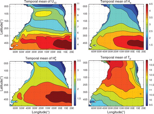
The time averages of and T _p have been computed at each grid point in the period from June 2006 to July 2007 (Fig. 1). The region with maxima wave height and wind velocity in the southeastern part of the Atlantic Ocean appear to be coupled with the values falling gradually towards north and approaching to the coasts. A similar pattern is observed in the swell average field, in line with Semedo et al. (2011). The peak period pattern shows a different aspect, with smaller values in the region of the most wave energy and increasing outwards from the main wave generation centre (Fig. 1).

Fig. 1.  Time averages of U ₁₀, given in m/s, H _s and , in meters and T _p , given in seconds, from June 2006 to July 2007.

5. Modes of variability

For each field analysed, we will present the four leading modes which explain most of the space-time variability. Table 1, shows the percentage explained by each of the four leading EOF's for the four fields considered.

Table 1. Fraction explained by the four EOFs for the four fields (in %)

	H s	U 10		T p
EOF1	38.2	11.8	39.6	28.6
EOF2	9.3	7.0	8.8	10.1
EOF3	7.1	5.4	6.9	7.8
EOF4	5.1	5.2	5.0	3.6
Total	59.7	29.4	60.3	50.1

We now present the individual modes of variability. These modes describe departures from mean patterns as presented in Section 4. In the Sections 5.1–5.5, we analyse the modes independently by means of empirical orthogonal functions. Some conclusions about the interdependence between the modes are drawn. In Section 5.6, we specifically examine the coupling between the modes by using SVDs and postulate some relationships between the patterns.

5.1. Significant wave height

The sum of the four leading modes has explained 59% of the entire H _s variance whose spatial patterns can be visualised in Fig. 2. The EOF₁(H _s ) exhibits a dominance with maximum value towards the southeast of the study area off shore from Southern Africa, spreading and waning toward the west and north. This pattern suggests a possible influence from the extratropical cyclonic actions that occur in the SA on the ocean wave. In fact, the region of higher positive variability coincides with the pattern III of extratropical cyclonic tracks in the SA according to the classification of Parise et al. (2009). The EOF₁(H _s ) matches the overall pattern of the first EOF of H _s presented in Sterl and Caires (2005) and also in Semedo et al. (2011). In both of these works, only the first mode of variability was presented and the EOF analysis was performed using wave data of ERA-40. However the short-scale pattern of the EOF₁(H _s ) given here presents a stronger positive anomaly, apart from being more diffuse over the SA. Semedo et al. (2011) performed an EOF analysis, using ERA-40, separately for the South Ocean and presented the percentages of variance due to the first two modes. The fraction of variability explained by the EOF₁(H _s ) (38.2%) in this work is within the limits obtained by Semedo et al. which are between 39%, for the months December–January–February and 33% for June–July–August.

Fig. 2.  Leading modes of variability of H _s .

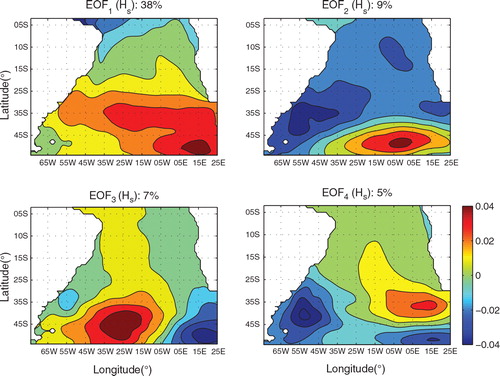
The second mode displays a dipole pattern where the positive and negative anomalies occur, respectively, on southeast and northwest while the EOF₃(H _s ) is characterized by a zonal pattern of wave action centres which has maintained the dipole structure, nevertheless, with positive anomalies in south/southwest, waning toward north and east. These modes have dipole structures, which is related to zonal changes in the location of the SA subtropical anticyclone, between the north and south directions (EOF₂(H _s )) and the east–west direction (EOF₃(H _s )). The fact that the imaginary line crossing the EOF₃(H _s )'s dipole is at 40S suggests that the variability accounted for by this mode could have oceanic origins associated with the Brazil–Malvinas Confluence.

The pattern EOF₃(H _s ) also represents the eastward propagating waves from the south pacific (SP). The fraction of variability accounted for by EOF₂(H _s ) is 9.3%, which is a value out of the interval [11.1%, 17.5%] given by Semedo et al. (2011). We conclude from this fact, and from the previous paragraph, that the EOF₁(H _s ) has had a distinct importance and that the wave dynamics was closer to unimodality, in the time period of study in this article.

Finally, the fourth leading mode of H _s displays three meridian bands of acting centres, one positive between two negative anomalies. The middle centre of action extends to north occupying most of the region analysed and is possibly related with swells between the two hemispheres, especially those coming from the NA which are more significant during the SA summer.

5.2. Surface wind speed

Among the four fields examined in this work, the variability explained by U ₁₀ was more evenly distributed between the EOF's. Furthermore, the amount explained by the first four EOF's is considerably less than the other cases; see Table 1.

The pattern of EOF₁(U ₁₀), shown in Fig. 3, presents mainly positive anomalies over the domain. A tripole structure can be recognised with centres of action off the coast of South Africa, South East of the American continent and in centre of the tropical SA. The same structure was observed in the EOF₁ of sea level pressure field obtained by Venegas et al. (1997) however with minimum values. The maximum positive anomaly in that paper corresponds to the main negative anomaly in the present work, located near 43S, 30W and shown by EOF₁(U ₁₀) in Fig. 3. EOF₂(U ₁₀) and EOF₃(U ₁₀) closely resemble the corresponding EOF's for H _s . This reflects the atmosphere–ocean forcing mechanism and the association with the SA subtropical anticyclone, mentioned in the previous subsection, is reinforced. Furthermore, the time variability of EOF₂(U ₁₀) is associated with the forcing mechanisms present in EOF₃(H _s ) and EOF₄(H _s ), as will become clear in Section 5.5.

Fig. 3.  Leading modes of variability of U ₁₀.

The fourth mode presents a tripole configuration with two opposite centres of action around 47S and a positive anomaly near 30S. This mode correlates, with opposite signs, with EOF₃(H _s ).

5.3. Swell

The modes of swell are shown in Fig. 4. EOF is similar to the EOF₁(H _s ). Nevertheless, the centre of action, near the South of Africa, is spread in all directions, over a larger region of the Atlantic. The spatial pattern of , apart from preserving a similarity with EOF₂(H _s ), presents a clear distinction between the east and west parts of the domain. The west is dominated by a strong negative anomaly separated from the positive variability in the east. The east–west dichotomy of is enhanced by the contribution of eastward propagating waves from the SP and by a well defined South of Africa action centre. The far east location of this centre of action suggests the influence from the swell field coming from the IO, in agreement with Alves (2006).

Fig. 4.  Leading modes of variability of .

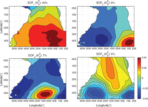
The third mode of variability of resembles the correspondent modes of H _s and U ₁₀ but does not present any positive anomaly in the northern domain. This fact, combined with the otherwise situation of the weaker modes, supports the orthogonal character of the leading modes.

spatial pattern is quite remarkable and appears only from the contribution of the NA generated swell. These waves extend over a large distance and cover almost the entire Atlantic Ocean. The contribution from the IO swell waves are absent in this mode. The swell shade can be clearly seen in this pattern which also provides an indication of its origin. This is connected with propagating swell waves from the north hemisphere (NH), during the winter in this hemisphere. The western SA is sheltered from these waves due to South American geography and this shading effect is clearly observed during the south hemisphere (SH) summer. See also the results by Semedo et al. (2011) where this swell shade appears in Fig. 7 obtained from an EOF analysis of only the months December, January and February.

5.4. Peak period

The four leading modes, accounting for 50% of the total variance, are shown in Fig. 5. EOF₁(T _p ) has a uniform polarity over the domain of study and is less dependent on the summer season than the other three field's leading EOF. This pattern could indicate the well-known swell waves incident to the west coast of Africa.

Fig. 5.  Leading modes of variability of T _p .

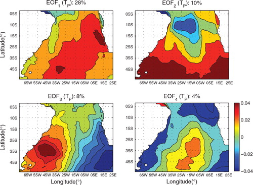
The second most important mode exhibits two latitudinal bands of centres of action with opposite signs. This is correlated with EOF, but with opposite signs.

EOF₃(T _p ) is strongly coupled, with signs reversed, with EOF. This forcing is supported by the time variability analysis that will be presented in Section 5.5. The EOF₃(T _p ) also suggests the influences of waves originating from the Pacific sector of the Southern Ocean and of the extratropical cyclones. The imaginary line joining the positions of the centres of action lies within the region of the tracks of these cyclones, in line with Parise et al. (2009).

The EOF₄(T _p ) displays a similar pattern with the EOF₃(U ₁₀) and also with EOF₃(H _s ) and that indicates a mechanism of a strong signal forcing a weaker signal.

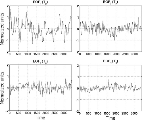
5.5. Time variability

The time series of the expansion coefficients of four variables are shown in Figs. 6–9. The time series of H _s , shown in Fig. 6, present oscillations in monthly and weekly time frames. In addition, the first principal component shows a seasonal dependence on the SH summer. The fluctuations in U ₁₀, in Fig. 7, are also monthly and weekly with a similar variation in the summer as depicted by the first time series. However, the spikes in the graphs are sharper and higher, as compared to the results for H _s and . The same conclusions of H _s time series could be stated for , whose time series shows roughly the same behaviour as the ones for H _s (Fig. 8). As we see in Fig. 9, the times series of the expansion coefficient of EOF₁(T _p ) exhibits a smaller dependence on the summer. The second and third time series of T _p resemble, with opposite signs, the fourth and second time series of , respectively. In fact, we could see these correlations from the corresponding spatial patterns, in Sections 5.3 and 5.4.

Fig. 6.  Time series of H _s . The horizontal axis represent the days in the time period from June 1996 to July 1997.

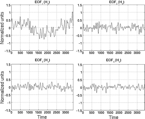
Fig. 7.  Time series of U ₁₀. The horizontal axis represent the days in the time period from June 1996 to July 1997.

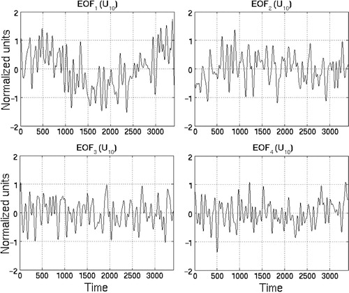
Fig. 8.  Time series of . The horizontal axis represent the days in the time period from June 1996 to July 1997.

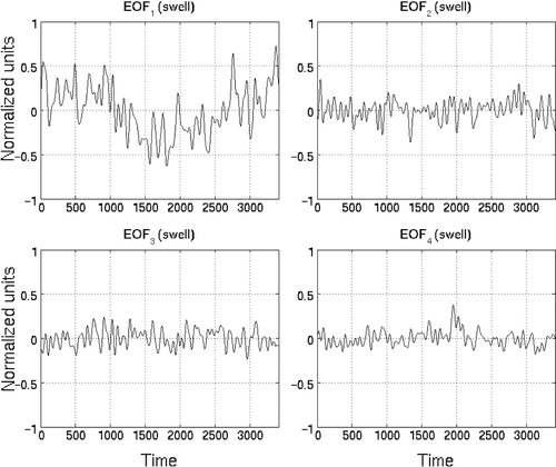
Fig. 9.  Time series of T _p . The horizontal axis represent the days in the time period from June 1996 to July 1997.

In Table 2, we show the correlation coefficients between the times series of all EOF modes. The coefficients with absolute values greater than 0.3 appear in bold font. The results in this table are relevant and very interesting. They confirm statements in the previous sections about the modes coupling and depict new aspects of the time correlation among the modes. In particular, we see not only strong correlation between H _s and in the diagonal of the block matrix defined by the crossing of these two variables, but also the strong influences of both variables second modes. The EOF₂(U ₁₀) has significant influence on the second, third and fourth modes of H _s . It is also noted here that there is an effective and strong coupling between with EOF₃(T _p ) and also between and EOF₂(T _p ).

Table 2. Correlation coefficients of the principal components

		H s								U 10
	EOF	1	2	3	4	1	2	3	4	1	2	3	4
	1	0.96	0.06	−0.09	0.02
	2	−0.08	0.64	−0.38	−0.31
	3	0.03	0.38	0.73	−0.17
	4	−0.05	0.34	−0.06	0.53
U 10	1	0.81	−0.26	0.04	−0.01	0.65	−0.21	−0.03	−0.21
	2	0.01	0.38	0.32	0.40	−0.06	−0.15	0.25	0.24
	3	0.17	0.48	0.08	0.14	0.19	0.00	0.20	0.16
	4	0.04	0.23	−0.65	0.04	0.08	0.22	−0.15	0.21
T p	1	0.64	0.08	−0.15	0.10	0.78	0.00	−0.13	0.18	0.19	−0.15	0.26	0.04
	2	0.39	0.19	0.06	−0.33	0.38	0.36	0.39	−0.41	0.33	−0.08	−0.02	0.09
	3	0.17	−0.21	0.33	0.22	0.13	−0.67	0.26	−0.07	0.15	0.40	0.08	0.07
	4	−0.07	0.39	0.17	0.13	−0.04	0.17	0.37	0.51	−0.27	−0.27	−0.02	0.05

5.6. Variability of coupled fields

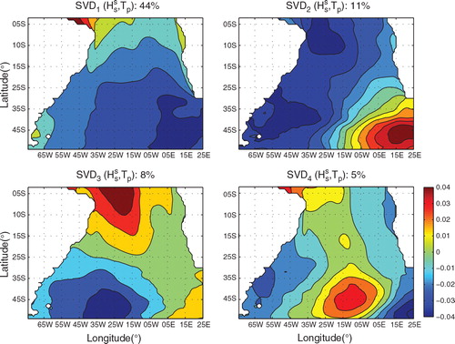
To further analyse and confirm the main relationships between the fields found in the previous subsections we now present the results of a SVD performed on the cross-covariance matrices between and T _p and between H _s and U ₁₀.

In contrast with the individual EOF modes of variability presented so far, the SVD analysis between two fields identifies only those modes in which the fields are coupled.

Figs. 10 and 11 show the spatial patterns of the four more significant SVD coupled modes between the variables and T _p . They explained 44%, 11%, 8% and 5%, respectively, of the total coupled variance. We observe that ≈ – . On the other hand, presents a pattern similar to – EOF₃(T _p ). Therefore, this mode is associated with the correlation found between and – EOF₃(T _p ). We also observe from these figures that ≈ – EOF₂(T _p ). This fact strongly supports the conclusion that this mode is related with the correlation already shown between modes EOF₂(T _p ) and – EOF.

Fig. 10.  SVD modes of associated to variations of T _p .

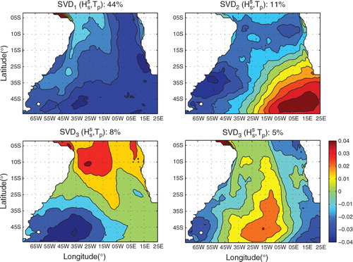
Fig. 11.  SVD modes of T _p associated to variations of .

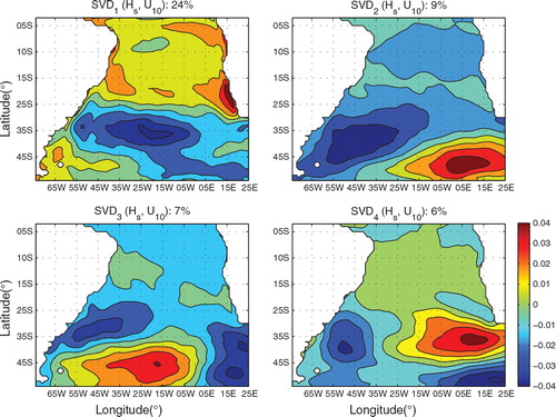
Let us now look at the SVD analysis between U ₁₀ and H _s . The four leading eigenvalues explained 24%, 9%, 7% and 6% of the total coupled variance. Fig. 12 shows the SVD modes of U ₁₀ associated with H _s . These two fields are strongly coupled and this is reinforced by the relationships found, namely SVD _i (U _10, H _s )≈ EOF _i (H _s ) for i=2, 3, 4 and SVD₁(U _10, H _s )≈ – EOF₁(H _s ). On the other hand, as depicted by Fig. 13, we observe that SVD₁(H _s, U ₁₀)≈ – EOF₁(U ₁₀) and SVD _i (H _s, U ₁₀)≈ EOF _i (U ₁₀) for i=2, 3. Note also that SVD₄(H _s, U ₁₀) has some similarity with EOF₂(U ₁₀), namely the dipole with a negative anomaly to a positive one between latitudes 35S and 45S. The pattern revealed by SVD ₄(H _s, U ₁₀) also shows a positive anomaly on the southeast near latitude 50S. This variation is present in EOF₄(H _s ). In fact, SVD₄(H _s, U ₁₀) represent the strong coupling between EOF₂(U ₁₀) and EOF₄(H _s ), as already demonstrated by the corresponding correlation coefficient between theses modes, in Table 2. This finding clearly depicts the atmosphere-to-ocean forcing by means of a strong signal forcing a weaker one.

Fig. 12.  SVD modes of U ₁₀ associated to variations of H _s .

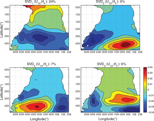
Fig. 13.  SVD modes of H _s associated to variations of U ₁₀.

6. Conclusions

The leading four modes of variability of H _s , , U ₁₀ and T _p in the SA have been computed and analysed by a short time scale simulation. Focusing on the time period of June 2006 to July 2007, and using high time resolution, detailed information about the region investigated was obtained. The individual leading modes contribution to the total variability ranged from 29%, in the case of U ₁₀, to up to 60%, for the H _s and .

The EOF analysis indicated that the main mode of H _s presents positive anomalies which are possibly associated with the extratropical cyclones in the SA. This indication is supported by the individual mode EOF₃(T _p ), which is correlated with and shows centres of actions in the region of the east–west changes in the tracks of such extratropical cyclones (Parise et al., 2009). We also identified a relationship between both the modes EOF₂(H _s ) and EOF₃(H _s ) with zonal changes in the location of the SA subtropical anticyclone.

We found that the H _s variance was strongly dominated by the first mode. Its eigenvalue alone explained 38.2% of the total significant wave height variability. Although this figure still falls within the range found by Semedo et al. (2011) in their recent study on the global wave climate using ERA-40, which is [33%, 39%] for the first EOF, we see the upper limit is practically achieved. However, if we look at the difference between the first and second eigenvalues of H _s , we come to the conclusion that the variance of H _s has been closer, in some sense, to unimodality. In fact, EOF₂(H _s ) has explained a fraction of only 9.3%, lying outside the range of the second EOF, obtained by Semedo et al., which is [11.1%, 17.5%].

The EOF₂(U ₁₀) and exhibit closer spatial similarity with the corresponding EOF's of H _s . Furthermore, we found that the time variability of EOF₂(U ₁₀) strongly correlates with that of EOF _i (H _s ), for i=2, 3, 4. The above mentioned aspects demonstrate identification of the atmosphere–ocean forcing. This forcing is also seen in other results in our study, namely, in the SVD analysis between the fields U ₁₀ and H _s , and appearing among the fields U ₁₀ and T _p , as indicated by the relation EOF₂(U ₁₀)≈EOF₄(T _p ).

As it is well-known, swell waves are intimately related to peak period. This kind of forcing is illustrated by relationships found in our study: and . Apart from the strong indication in the EOF spatial patterns, these associations are supported by the time variability analysis and by the coupled variability's shown by the SVD.

We observed a well-defined and persistent negative anomaly in the to the west of the SA. This swell shade is generated by swell waves propagating from the NH during the winter in this hemisphere and appears in a region which is blocked from these waves as a result of the geography of South America. This is clearly seen in and also in EOF₂(T _p ). These results corroborate with long-scale results by Semedo et al. (2011).

Acknowledgements

The first author acknowledges financial support from CNPq and the second author has done part of the research on this article while a member of the EU project FP7-295217 – HPC-GA.

References

- Alves, J. H. G. M1999. On the measurement of directional wave spectra at the southern Brazilian coast. Appl. Ocean Res. 21(6), 295–309. doi:10.3402/tellusa.v64i0.17362.
- Alves J. H. G. M. Numerical modeling of ocean swell contributions to the global wind-wave climate. Ocean Modelling. 2006; 11: 98–122. 10.3402/tellusa.v64i0.17362.
- Branco F. V. Contributions of Swells Generated by Distant Storms to the Wave Climate of Brazil's Coast. Master Thesis. USP, São Paulo, Brazil. In Portuguese.2005
- Branco, F. V, Alves, J and Camargo, R. 2004. Contribuies de swell gerado em tempestades distantes para o clima de ondas na costa brasileira. Brazilian Congress of Meteorolog. Fortaleza: Brazil.
- Caires S. Sterl A. 100-year return value estimates for ocean wind speed and significant wave height from the era-40 data. 2005; 18: 1032–1048. 10.3402/tellusa.v64i0.17362.
- Cavalcanti, I. F. A, Marengo, J, Satyamurty, P, Nobre, C. N, Trosnikov, I and co-authors. 2002. Global climatological features in a simulation using the cptec/cola agcm. J. Clim. 15(21), 2965–2988.
- Cheng X. Dunkerton T. J. Orthogonal rotation of spatial patterns derived from singular value decomposition analysis. Clim. Dyn. 1995; 8: 2631–2643.
- Gulev S. K. Grigorieva V. Last century changes in ocean wind wave height from global visual wave data. J. Clim. 2004; 31: L24302.10.3402/tellusa.v64i0.17362.
- Gulev S. K. Grigorieva V. Variability of the winter wind waves and swell in the North Atlantic and North Pacific as revealed by the voluntary observing ship data. Geophys. Res. Lett. 2006; 19: 5667–5785. 10.3402/tellusa.v64i0.17362.
- Hemer M. A. Church J. A. Hunter J. R. Variability and trends in the directional wave climate of the Southern Hemisphere. J. Clim. 2010; 30(4): 475–491.
- Komen G. J. Hasselmann S. Hasselmann K. On the existence of a fully developed wind-sea spectrum. Int. J. Climatol. 1984; 14: 1271–1285.
- Komen, G. J, Cavaleri, L, Donelan, M, Hasselmann, K, Hasselmann, S and Janssen, P. A. E. M. 1994. Dynamics and Modelling of Ocean Waves. Cambridge University Press. ISBN-10: 0521577810.
- Marengo, J, Cavalcanti, I. F. A, Satyamurty, P, Trosnikov, I, Nobre, C. N and co-authors. 2003. Assessment of regional seasonal rainfall predictability using the cptec/cola atmospheric gcm. Clim. Dyn. 21(5), 459–475. 10.3402/tellusa.v64i0.17362.
- Mendona A. M. Bonatti J. P. Experiments with EOF-based perturbation methods and their impact on the cptec/inpe ensemble prediction system. Mon. Wea. Rev. 2009; 137: 1438–1459. 10.3402/tellusa.v64i0.17362.
- Panetta, J, Barros, S. R. M, Bonatti, J. P, Tomita, S and Kubota, P. Y. 2007. Computational cost of cptec agcm. Use of High Performance Computing in Meteorology. Reading: UK, pp. 65–83.
- Parise, C. K, Calliari, L. J. and N. Krusche, N. 2009. Extreme storm surges in the south of Brazil: atmospheric conditions and shore erosion. Braz. J. Oceanogr. 57(3), 175–188. 10.3402/tellusa.v64i0.17362.
- Pianca C. Mazzini P. L. F. Siegle E. Brazilian offshore wave climate based on NWW3 reanalysis. Braz. J. Oceanogr. 2010; 58(1): 53–70. 10.3402/tellusa.v64i0.17362.
- Semedo A. Suseli K. Turgersson A. Sterl A. A global view on the wind data and swell climate and variability from era-40. J. Clim. 2011; 24: 1461–1479. 10.3402/tellusa.v64i0.17362.
- Sterl A. Caires S. Climatology, variability and extrema of ocean waves: the web-based knmi/era-40 wave atlas. Int. J. Climatol. 2005; 25: 963–977. 10.3402/tellusa.v64i0.17362.
- Swail V. R. Cox A. T. On the use of ncep-ncar reanalysis surface marine wind fields for a long-term North Atlantic wave hindcast. J. Atmos. Oceanic Tech. 2000; 17: 532–545.
- Thomson, R. E and Chow, K. Y. 1980. Butterworth and lanczos-window cosine digital filters: With application to data processing on the univac 1106 computer. Technical report. Institute of Ocean Science: Sydney.
- Venegas S. A. Mysak L. A. Straub D. N. Atmosphere-ocean coupled variability in the South Atlantic. J. Clim. 1997; 10: 2904–2920.
- Violante-Carvalho, N, Parente, C. E, Robinson, I. S and Nunes, L. M. P. 2002. On the growth of wind-generated waves in a swell-dominated region in the South Atlantic. J. Offshore Mechanics Arctic Eng.-Trans. ASME. 124(1), 14–21. 10.3402/tellusa.v64i0.17362.
- Wang X. L. Swail V. R. Changes of extreme wave heights in Northern Hemisphere oceans and related atmospheric circulation regimes. J. Clim. 2001; 15: 2204–2221.
- Wang X. L. Swail V. R. Trends of Atlantic wave extremes as simulated in a 40-yr wave hindcast using kinematically reanalyzed wind fields. J. Clim. 2002; 15: 1020–1034.
- Woolf D. K. Challenor P. G. Cotton P. D. Variability and predictability of the North Atlantic wave climate. J. Geophys. Res. – Oceans. 2002; 107(10): 3145.10.3402/tellusa.v64i0.17362.
- Young I. R. Zieger S. Babanin A. V. Global trends in wind speed and wave height. Science. 2011; 332: 451–455. 10.3402/tellusa.v64i0.17362.