Control of lateral boundary conditions in four-dimensional variational data assimilation for a limited area model

ABSTRACT

The limited area model forecasting problem is a lateral boundary condition (LBC) problem in addition to the initial condition problem. The data assimilation has traditionally been considered as a process for estimation of the initial condition only, while for the limited area data assimilation this estimation may be extended to include also the LBCs, at least during the data assimilation time window when observations are available. A procedure for such a control of the LBCs has been included in the four-dimensional variational data assimilation (4D-Var) scheme for the HIgh Resolution Limited Area Model (HIRLAM) forecasting system. A description of this procedure is provided together with results from idealised as well as real data experiments. The results indicate that control of LBCs may be important with small forecast domains and in particular for weather disturbances moving quickly into and through the forecast domain.

• data assimilation
• lateral boundary conditions

1. Introduction

The limited area model (LAM) forecasting problem is a lateral boundary condition (LBC) problem in addition to the initial condition problem. For numerical weather prediction, the LBCs are generally provided by a host model, for example, a global numerical weather prediction model. One may argue that the available boundary conditions from the host model have to be accepted without change for usage in the LAM. However, one may use the observations close to the lateral boundaries and let these influence the initial conditions. In case if the initial conditions are used as the LBCs at the initial time, the subsequent forecast will also be influenced by these observations. With application of four-dimensional variational (4D-Var) data assimilation for the LAM forecasting, a bit more is possible since the LBCs during the period of the data assimilation window may be controlled. This may be particularly important for assimilation of phenomena that are observed well inside the LAM domain during the later part of the data assimilation window, while being propagated through the lateral boundaries during the early part of the data assimilation window. If we do not control the LBCs at the end of the data assimilation window, observed information related to these phenomena during the later part of the data assimilation window may be lost and worsen the subsequent forecast inside the domain.

The review process was handled by Harald Lejenás, Editor-in-Chief.

For the control of the LBCs in an LAM 4D-Var data assimilation, the tangent linear and adjoint versions of the schemes for the coupling to the larger scale model providing the LBCs are needed. Errico et al. (1993) applied the adjoint of the coupling scheme in an LAM to investigate the sensitivity of LAM forecast errors to initial as well as LBCs. A similar study was carried out by Gustafsson et al. (1998) for a significant storm development over the North Atlantic, indicating the importance of controlling the lateral boundaries in such cases and, in particular, for small forecast domains. The experiments of Gustafsson et al. (1998), using the adjoint of the Davies (1983) lateral boundary relaxation, also provided some insight into the need for controlling noise associated with adjustment processes in the lateral boundary relaxation zone.

For the control of the LBCs in the Japan Meteorological Agency (JMA) mesoscale LAM 4D-Var, Kawabata et al. (2007) introduced a full model state control variable for the LBCs at the end of the assimilation window and a 4D-Var cost function constraint for this new lateral boundary control variable. This constraint had a similar form as for the background error constraint, but no further documentation about the JMA approach is available (Kawabata, personal communication, 2012). For the control of LBCs in the HIgh Resolution Limited Area Model (HIRLAM) 4D-Var, we have followed the JMA approach and a similar approach has also been taken at NCAR for the WRF model 4D-Var (Xin Zhang, personal communication, 2011). A different approach has been taken for the control of LBCs in the Canadian Regional Prediction System (Luc Fillion, personal communication, 2011) by extending the model domain for the tangent linear and adjoint model integrations in comparison with the domain for the non-linear model.

Related to the control of LBCs in an LAM 4D-Var is the inherent difficulty to account for such larger scale forecast errors that can neither be represented without aliasing effects by spectral error components over the limited area domain (Baxter et al., 2011) nor by the observations within the model domain. One possibility is to rely on larger scale models, preferably global models, to handle these large-scale forecast errors and to constrain these larger scales to the output of larger scale models during the LAM data assimilation. Guidard and Fischer (2008) applied such an explicit large-scale error constraint, constraining the larger scales to a global analysis, within a 3D-Var LAM analysis. Dahlgren and Gustafsson (2012) applied a similar constraint within the HIRLAM 4D-Var assimilation, constraining the larger scales to a global short-range (+3 h) forecast, thereby avoiding the difficulty of using observations twice as in the case of constraining the larger scales with global analysis data. It may be hypothesised that an optimal 4D-Var for an LAM should apply control of LBCs as well as a large-scale error constraint, but this falls beyond the scope of the present study.

The algorithms for control of LBCs are described in section 2 of this article, followed by section 3 on the derivation of statistics needed for one of the algorithms. After that we provide some illustrations giving the performance of the algorithms in the form of single simulated observation impact experiments in section 4. The results of real observation assimilation experiments are given in section 5, and discussion and concluding remarks are included in section 6.

2. Formulation of the LBC constraint in the HIRLAM 4D-Var

2.1. The HIRLAM 4D-Var

The HIRLAM 4D-Var (Gustafsson et al., 2012) is based on the incremental approach suggested by Courtier et al. (1994). The assimilation control variable is formulated in spectral space (Gustafsson et al., 2001) with a background error constraint similar to the one described by Berre (2000). The model domain extension of Haugen and Machenhauer (1993) is applied to obtain periodic variations in both horizontal directions, needed for the spectral transforms. Furthermore, the minimisation is given a multi-incremental formulation (Veersé and Thépaut, 1998), providing the possibilities for forecast model and observation operator re-linearisations during the minimisation. A weak digital filter constraint (Gustafsson, 1992; Gauthier and Thépaut, 2001) is also applied to minimise the growth of fast gravity wave oscillations. The simplified physics package of Janisková et al. (1997) has been implemented in the tangent linear and adjoint models of the HIRLAM 4D-Var; only the turbulence parameterisation of this package is applied in the present study.

2.2. Control of lateral boundary conditions

The control variables and the constraints for control of LBCs that we will apply in this study can be considered as special cases of a model error constraint applied in a weak constraint 4D-Var (Trémolet, 2006), see section 2.3. For the description of the control of LBCs in HIRLAM 4D-Var, we will, however, follow Kawabata et al. (2007) and we introduce the LBC perturbations as a control variable at the end of the data assimilation window (time t_K). For the lateral boundary increment at the start of the assimilation window (time t₀), we will use the initial condition increment . For intermediate time steps during the integration of the tangent linear model, we will obtain the LBCs by the same linear time interpolation scheme that is used in the non-linear model. Once the LBCs are defined, the same lateral boundary relaxation scheme that is used in the non-linear model (Davies, 1983) can also be used in the tangent-linear model, and the adjoint of the lateral boundary relaxation is also well defined, see Gustafsson et al. (1998). Note, however, that while the LBCs are input perturbation data to the tangent linear model, the LBCs are output error gradient data from the adjoint model.

Again, following Kawabata et al. (2007), we will introduce a cost function term J_lbc that will measure the distance to the unperturbed LBCs used in the non-linear model1

where represents the covariance of the LBC errors at the end of the data assimilation window (time t_K). LBCs only need to be defined in the narrow lateral boundary zone, but it would be difficult to specify the proper spatial scales and balances representing the LBC errors over such a narrow domain. We have therefore made the choice to specify the lateral boundary control variable over the same total model domain as the initial condition control variable. Since both of these control variables represent forecast errors, albeit for different forecast lengths and possibly for different models, it is clear that their respective error covariance can be represented in a similar way. In a first trial to test the sensitivity of the assimilation to the control of the LBCs, we will simply apply = . Note, however, that while the LBC control variable is representing the full model domain, the adjoint (error gradient) of the control variable will be forced in the lateral boundary relaxation zone only during the adjoint model integration.

One potential problem for the LBC constraint in the form described previously is that the LBC errors at the end of the assimilation window may be strongly correlated with the initial condition errors at the start of the assimilation window. If such correlations are not handled properly, the solution of the minimisation problem may become suboptimal.

One simple pre-conditioning would be to subtract the LBCs at the start of the assimilation window from the LBCs at the end of the assimilation window, thus to treat the tendency of the LBCs over the data assimilation window () as the control variable and to apply the following cost function constraint:2

This approach would also require the covariance of forecast tendency errors that could be possibly estimated by the NMC1 method (Parrish and Derber, 1992) from differences between forecast tendencies valid at the same time.

In the following we will compare the two described methods for controlling the LBCs in real observation data assimilation experiments. We will also compare with the case of not controlling the LBCs and with the case of controlling the LBCs only at the start of the data assimilation window. For the second approach of controlling the LBCs, we will also derive the needed error statistics for LBC tendency errors by the NMC method. The full model state error statistics and the model state tendency error statistics will also be compared and discussed.

For clarity, here we will summarise the four different methods that we will compare and validate in this study:

• Method nolbc1 without control of LBCs and with the LBCs at the start of the assimilation window equal to zero ().

• Method nolbc2 without control of LBCs and with the LBCs at the start of the assimilation window equal to the initial condition increments (, ).

• Method lbc1 with control of the LBCs at the end of the assimilation window (, is controlled and constraint (1) is applied).

• Method lbc2 with control of the tendency of the LBCs over the assimilation window (, , is controlled and constraint (2) is applied).

2.3. A note on the similarity with the model error constraint

A weakness of the basic HIRLAM 4D-Var formulation is the assumption of a perfect forecast model that propagates the assimilation increment over the data assimilation window. As a first simple remedy, the possibility to estimate a systematic model tendency error, , constant in time over the assimilation window but variable in space over the model domain, has been introduced into the HIRLAM 4D-Var. This model tendency error term is added to the calculated model tendency during the integration of the tangent linear model. To estimate this model tendency error, is added to the control vector and a model error constraint J_me is added to the assimilation cost function:3

There is a strong similarity between the model error constraint and the pre-conditioned LBC constraint, described previously (method lbc2). The LBC constraint acts like a model error constraint, where the corresponding adjoint control variable is forced by error gradient information in the lateral boundary zone only. Thus, the model error constraint could be regarded as a generalisation of the LBC constraint. The covariance of the model error could be estimated in the same way as discussed earlier for the LBC error covariance. Note that the model error constraint, as described here, is not applied in the present study; it is only mentioned to note the similarity with the second form of the LBC constraint.

3. Derivation of lateral boundary condition error statistics

For application of the control of LBCs in the pre-conditioned form such that the tendency of the LBCs is the control variable, we need statistics to include in the corresponding error covariance matrix . The LBCs are generally obtained from a larger scale global forecast model, in the case of forecasting with HIRLAM global operational forecasts from ECMWF are used. It may be argued that LBC error statistics should be derived from the time history of the host model forecasts. On the other hand, the LBC errors do affect all modelled scales of the LAM, because they are one aspect of model errors in an LAM. For this reason, we made the choice to derive the needed LBC error statistics from historical HIRLAM data.

Background error statistics (the -matrix) for HIRLAM may either be derived by the NMC method (Parrish and Derber, 1992), where differences between forecasts of different lengths valid at the same time are taken as proxies for short-range forecast errors, or by the method of Ensemble of Data Assimilations (EDA) (Houtekamer et al., 1996), where perturbation of observations is the core of the ensemble generation process. The background error statistics for the reference HIRLAM are based on the NMC method (Gustafsson et al., 2001), and we made the choice to derive the LBC error statistics also by the NMC method.

To have consistent sets of statistics for the background errors and for the LBC errors, we derived both of these sets of statistics from the same winter period (January–March 2011) of reference HIRLAM forecasts. We made the choice for a winter period since the data assimilation experiments are carried out for a winter period and since, for example, background error variances, background error vertical correlations and multivariate balance constraints with moisture involved are quite seasonally dependent. The background error statistics were derived from the differences between +36 h and +12 h forecasts, initialised at 00 UTC and valid at the same time. Similarly, the LBC tendency error statistics were derived from differences between 5 h forecast tendencies (from +36 h to +41 h) and 5 h forecast tendencies (from +12 h to +17 h) valid for the same time interval and taken from forecasts initialised at 00 UTC. The choice of a 5 h interval for the tendency calculation was motivated by the assimilation time window in the standard HIRLAM 4D-Var (for the 00 UTC assimilation cycle, for example, observations from the interval 20.30 UTC until 02.30 UTC are collected in hourly observation time windows from 21 UTC until 02 UTC, and thus, the tangent linear and adjoint models have to be integrated over a 5 h time interval).

Details on the derivation of background error statistics are given in Berre (2000). Horizontal correlations are handled in spectral space, assuming that the different spectral components are de-correlated. Implicitly, this means that horizontal homogeneity is assumed with respect to horizontal correlations.

We will illustrate here the main characteristics of the differences between background forecast error statistics and forecast tendency error statistics estimated by the NMC method, and we will take statistics for vorticity as an example. The derived standard deviations (SDs) for vorticity forecast differences and vorticity forecast 5-h tendency differences as functions of vertical level are presented in Fig. 1. The SDs for the forecast 5-h tendency differences are significantly larger than the SDs for forecast differences with a factor of in the middle troposphere. Essentially, this means that vorticity forecast differences are only weakly correlated over 5 h in time. For the variance of the 5-h tendency of any quantity , we will have

Fig. 1.  Standard deviations of differences between vorticity forecasts valid at the same time (dotted lines) and SDs of differences between 5-h vorticity forecast tendencies valid at the same time (full lines), both given as functions of the vertical level.

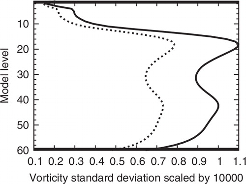
where VAR and COV denote variance and covariance, respectively. In case of complete de-correlation in time, and assuming the same variance of the vorticity forecast differences for different times of the day, the SD for the forecast 5-h tendency difference would be a factor larger than the SD for the forecast difference.

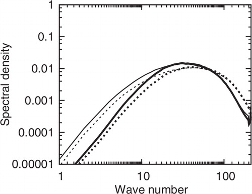
Of crucial importance for the performance of the data assimilation process are the assumed horizontal spectral densities for the different model variables, corresponding to the horizontal auto-correlations in physical space. We have included the horizontal autocorrelation spectra for vorticity forecast differences, as well as for vorticity forecast 5-h tendency differences, on model levels 30 (500 hPa) and model level 50 (850 hPa) in Fig. 2. We may notice a shift towards smaller horizontal scales in the spectral density for the forecast 5-h tendency differences in comparison with the forecast differences. This is an indication of the importance of the smaller scales in the forecast model 5-h tendency field, mainly due to a stronger correlation in time over 5 h for the larger scales.

Fig. 2.  Horizontal variance spectra normalised with the total variance for differences between vorticity forecasts valid at the same time (thin lines) and for differences between 5-h vorticity tendencies valid at the same time (thick lines). Model level 30 (500 hPa, full lines) and model level 50 (850 hPa, dotted lines).

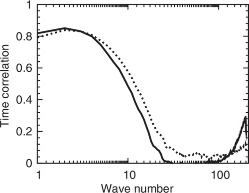
From the information in Figs. 1 and 2, the time correlation of forecast differences over 5 h as a function of horizontal wave number may be calculated. We have included in Fig. 3, the estimated time correlation for vorticity forecast differences as a function of horizontal wave number for model levels 30 and 50. For waves longer than wave number 10 (wave length 1000 km), we can notice a strong correlation in time (of the order 0.40–0.85). However, the forecast vorticity difference is dominated by smaller scales (Fig. 2) that are not correlated in time (Fig. 3). This scale dependency of forecast difference time correlations can be understood from the importance of advective processes over a few hours. Considering a similar advection velocity, shorter waves will be advected much quicker over a full period of the wave. The increased time correlation at the shortest horizontal scale may possibly be interpreted as the effect of stationary waves forced by orography and coupled to the larger scale waves. The statistics for these shorter scale horizontal waves do not influence the assimilation results strongly, since a wave with wave number 100, in which an increase in the time correlation is noticed, corresponds to a wavelength of 100 km for which the spectral energy is relatively small (Fig. 2). Furthermore, the shortest resolved wave in the 4D-Var increments that we are going to apply is of the order 66 km. The time correlation for unbalanced temperature, one of the assimilation control variables, was also investigated. The dependency of the time correlation for unbalanced temperature on horizontal scale in the middle troposphere was similar as for the time correlation for vorticity at the same levels. The time correlation for unbalanced temperature close to the surface of the earth behaved differently with larger time correlations also for smaller horizontal scales. This may be an indication of stationary temperature waves forced by the lower boundary, although one needs to be a bit careful with such an interpretation since the analysis in spectral space is based on the assumption of horizontal homogeneity with respect to horizontal correlations.

Fig. 3.  Time correlation of vorticity forecast differences at model level 30 (500 hPa, full line) and model level 50 (850 hPa, dotted line).

For the 4D-Var assimilation with control of LBCs at the end of the data assimilation window (method lbc1), we may hypothesise that due to the weak correlation in time of vorticity increments (modelled here using vorticity forecast differences) the minimisation would result in an optimal solution and also be reasonably well conditioned. Furthermore, in case if the LBC tendency would be used as an assimilation control variable (method lbc2), proper statistics for tendency increments need to be applied. We will test these hypotheses through practical data assimilation experiments.

4. Single simulated observation impact experiments

Since the idea of controlling LBCs in meteorological data assimilation is quite new, without any details presented so far in the literature, we find it useful to illustrate the basic mechanisms of such an LBC control through so-called single observation impact experiments. For this purpose, we may place a single simulated observation in a position close to the lateral boundaries, possibly at different physical distances from the lateral boundary and for different inflow and outflow conditions.

Before showing the results, it is needed to note some details of the numerical formulations of the data assimilation and forecast system. Both the HIRLAM grid point forecast model and the tangent linear and adjoint spectral models of the HIRLAM 4D-Var are based on two time-level semi-Lagrangian semi-implicit time integration schemes. The coupling to the host model is carried out with ‘lateral boundary relaxation’ as proposed by Davies (1983), slightly modified to fit the needs of the long time steps of the semi-Lagrangian time integration scheme. The model domain can be divided into three different subdomains: (1) the passive boundary zone closest to the lateral boundaries where the model solution is given fully by the host model—this zone has been included to ensure that semi-Lagrangian trajectories do not pass through the lateral boundaries; (2) the boundary relaxation zone where the model solution every time step is relaxed towards the host model solution with a relaxation weight for the host model decreasing with distance from the lateral boundary and (3) the inner domain where the model solution is fully given by the LAM equations. Finally, LBCs are provided at certain time intervals, for example, every 6 or every 3 h, and a simple linear time interpolation is applied to obtain LBCs for time steps in between.

For the experiment with single simulated observations, we applied the non-linear model at 20 km horizontal resolution, while the tangent linear and adjoint models of the 4D-Var minimisation were applied at 40 km horizontal resolution. The width of passive boundary zone was set to be 80 km and the width of the boundary relaxation zone was set to be 200 km for the tangent linear and adjoint model integrations.

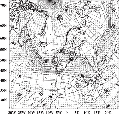
A model domain and an experimental case were taken to be the same as described by Gustafsson et al. (2012) for 4D-Var single simulated observation experiments. The model domain and the model level 15 (300 hPa) wind background state for 3 December 1999 00UTC + 6 h are illustrated in Fig. 4. 4D-Var data assimilation was carried out over the assimilation time window 3 December 1999 06UTC-11UTC.

Fig. 4.  The model level 15 (300 hPa) wind background field, 3 December 1999 00UTC +6 h, applied during the single observation impact experiments. The contour interval is 10 m s⁻¹.

From a data assimilation point of view, one of the most interesting scenarios for testing the control of LBCs are cases when we have a strong inflow over the lateral boundaries and with observations provided inside the domain close to the lateral boundaries and at observation times being close to the end of the 4D-Var data assimilation window. Such cases cannot be handled well with control of initial conditions only since the needed meteorological signal may be positioned well outside the lateral boundaries at the start of the data assimilation window. We may say that inflow of observed information in the forward non-linear and tangent-linear models becomes outflow of error gradient information during the backwards integration of the adjoint model in the 4D-Var minimisation process.

We selected the area of strong inflow around 30°N, 15°W for our single observation impact studies and carried out experiments with single observations valid at 3 December 1999 11 UTC (5 h into the data assimilation window) and positioned at (1) 30°N, 12°W, 80 km from the lateral boundary and inside the passive boundary zone and at (2) 32°N, 12°W, approximately 300 km from the lateral boundary and inside the inner model domain. The observed value that was simulated was a south-westerly wind increment of 9 m s⁻¹ (= 4 m s⁻¹ and = 8 m s⁻¹) at 300 hPa, associated with an observation error SD of 2 m s⁻¹.

Here, we will show results from observations in the second position only. With observations in the first position, in the passive boundary zone, the only model process that could affect the data assimilation is the linear time interpolation of the lateral boundaries between +00 h and +05 h in the data assimilation window. Since the observation was taken at +05 h (11 UTC), the minimisation simply introduced a smooth increment into the LBC increment field valid at this time, when the control of lateral conditions was applied in the 4D-Var minimisation. In case if no control of lateral conditions was applied, the minimisation provided only zero-valued assimilation increments.

For the case with the simulated observation in the second position and control of LBCs (with method lbc1), wind assimilation increments at model level 15 (300 hPa) are presented for +0 h, +3 h and +5 h into the data assimilation window in Fig. 5. We may notice a smoothly varying assimilation increment that is moving towards north-east during the 5-h data assimilation window, with a maximum increment of approximately 5.5 m s⁻¹ at +5 h in the vicinity of the simulated observation at 32°N, 12°W.

Fig. 5.  Model level 15 wind field assimilation increments from a simulated south-westerly wind observation increment of 9 m s⁻¹ at 3 December 1999 11UTC in the position 32°N, 12°W (marked OBS). With control of lateral boundary conditions (method lbc1). 3 December 1999 06 UTC (upper), 09 UTC (middle) and 11 UTC (lower). The contour interval is 1 m s⁻¹.

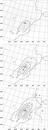
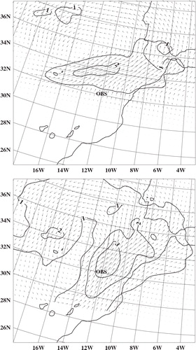
The same single observation impact experiment was repeated, but now without control of the LBCs (method nolbc1). In this case, the 4D-Var minimisation completely failed to adjust the initial data such that the tangent linear model would fit the simulated observation increment at +5 h. The reason is quite clear from the assimilation increment at +3 h, in the middle of the data assimilation window; see Fig. 6 (upper). All relevant increment information has completely been wiped out from the passive boundary and the boundary relaxation zones, since boundary conditions both at the start and at the end of the data assimilation window are assumed to be zero for the tangent linear model integrations in the standard HIRLAM 4D-Var. The results are slightly improved at +3 h (Fig. 6, lower) in case the boundary conditions for the tangent linear model integration at the start of the data assimilation window are taken to be the initial time assimilation increments (method nolbc2), a solution chosen for the WRF 4D-Var (Xin Zhang, personal communication, 2011). However, at +5 h when the simulated observation was chosen to influence the data assimilation, the assimilation increments were equally poor with the two versions of treating the initial boundary conditions due to the full effect of the zero LBCs at the end of the data assimilation window (figure is not shown). A proper assimilation of the simulated observation in this case can only be achieved through control of the LBCs at the end of the data assimilation window.

Fig. 6.  Model level 15 wind field assimilation increment at 3 December 1999 09 UTC from a simulated south-westerly wind observation increment of 9 m s⁻¹ at 3 December 1999 11UTC in the position 32°N, 12°W (marked OBS), without control of lateral boundary conditions. Zero-valued lateral boundary conditions at the initial time (method nolbc1, upper), lateral boundary conditions at the initial time equal to the initial condition increments (method nolbc2, lower). The contour interval is 1 m s⁻¹.

To check the dependency on the flow situation along the lateral boundaries, a simulated observation was placed at 32°N, 7°W, in an area with a weaker inflow in the background state. In this case, a larger part of the observed increment was reflected in the initial increments and a tendency for creating a double structure in the maximum of the assimilation increment was noticed. This is most likely caused by the simple linear interpolation in time between the LBC increment fields valid at +0 h and +5 h. Thus, it may be appropriate to increase the time resolution of the LBCs to be controlled. Indeed, this was one of the reasons for choosing an alternative technique for controlling the LBCs for the Canadian regional 4D-Var (Luc Filion, personal communication, 2011).

5. Real observation assimilation experiments with and without control of LBCs

5.1. The model and data assimilation setup

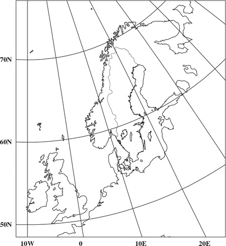
To validate the impact of the LBC constraint in HIRLAM 4D-Var, experiments with all four methods described in section 2 (nolbc1, nolbc2, lbc1 and lbc2) were carried out for a period of one month. The period of December 1999 was selected since this month was characterised by several mesoscale storm developments over Europe. HIRLAM 4D-Var with a single outer loop iteration was applied and the experiments were done for the operational SMHI 11 km HIRLAM domain, see Fig. 7, and with 60 vertical levels. The operational SMHI 11 km HIRLAM domain includes 256×288 horizontal grid points. This relatively small forecast domain was chosen on purpose in order to maximise the possibilities to find an impact from controlling the LBCs. The HIRLAM grid point forecast model applies a two-time level semi-Lagrangian semi-implicit time integration scheme (Undén et al., 2002). The physical parameterisations include the CBR turbulence scheme (Cuxart et al., 2000), the Kain-Fritsch convection scheme (Kain, 2004), the Rasch-Kristjánsson cloud water scheme (Rasch and Kristjánsson, 1998), the simplified radiation scheme of Savijärvi (1990) and the ISBA surface and soil scheme (Noilhan and Mahfouf, 1996). LBCs were obtained from forecasts available at 00UTC and 12UTC in the ECMWF ERA-40 re-analysis data sets (Uppala et al., 2005). The HIRLAM 4D-Var was applied with a horizontal increment resolution of 33 km and with a 6 h data assimilation cycle. Forecasts up to +36 h were produced at 00UTC and 12UTC.

Fig. 7.  The SMHI 11 km data assimilation and forecast domain.

5.2. Forecast verification results

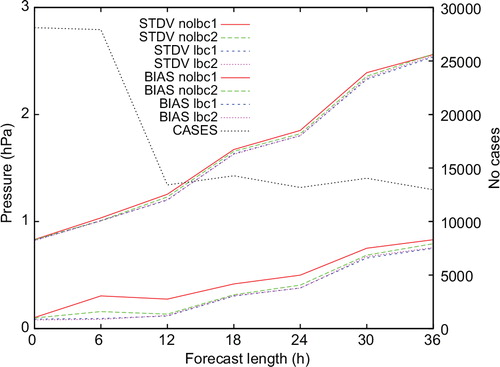
The forecasts produced by the experiments were verified against SYNOP surface observations and against radiosonde profile observations. Forecast mean error (BIAS) and SD are presented instead of root mean square error (RMSE) since RMSE is strongly influenced by the BIAS. All verification scores showed a small positive or a neutral impact of the control of LBCs. Fig. 8 shows verification of mean sea level pressure forecasts as verified against SYNOP observations within a Scandinavian domain and averaged over the whole month of December 1999. The verification scores are given as functions of forecast length. A small but systematic positive impact of the control of lateral boundaries can be seen for all forecast lengths. It is, however, not possible to separate the verification scores for the two experiments with slightly different techniques for controlling the LBCs. Note also that the forecast verification scores for the experiment (nolbc2) without control of LBCs at the end of the data assimilation window, but with the LBCs at the start of the assimilation window equal to the initial condition increments falls in between the forecast verification scores for the other experiments.

Fig. 8.  BIAS (mean error) and SD (standard deviation of error) verification scores for mean sea level pressure forecasts over a Scandinavian domain as verified against SYNOP observations for the forecast lengths +0 h, +6 h, +12 h, +18 h, +24 h, +30 h and +36 h. Verification scores are averaged for the month of December 1999. Experiments nolbc1 (red lines), nolbc2 (green lines), lbc1 (blue lines) and lbc2 (pink lines). Grey line marked CASES shows the number of verifying observations.

A closer look at time series of mean sea level pressure verification scores (figures are not shown) revealed that the positive impact originates from a few isolated and short time periods, for example, for +36 h forecasts valid 4 December 1999 12 UTC and 6 December 1999 12 UTC. The strongest impact was seen for the second of these two cases and this case will be further investigated below. The impact on the forecast valid 4 December 1999 12 UTC is also of interest since it was related to the intensity and position of a very strong mesoscale storm that hit Denmark and Southern Sweden (the ‘Denmark storm’).

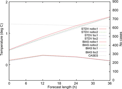
Scores for verification of relative humidity forecast profiles against radiosonde observations are included in Fig. 9. We may notice a small positive impact of the control of the LBCs but no distinguishable difference in forecast scores from the two experiments testing the different versions of the control of lateral boundaries. By looking at the verification scores for 500 hPa temperature as a function of forecast length (Fig. 10) over a European domain we see a clear increase in the SD (standard deviation of error) verification scores at forecast length 0 h for the experiments without control of lateral boundaries in comparison with the experiments with control of lateral boundaries. This should be interpreted as a difficulty for the assimilation to adapt to observations close to the lateral boundaries, a similar feature that we already noticed through the single simulated observation experiments. Repeating the verification of 500 hPa temperature against radiosonde observations from a Scandinavian domain in the centre of the model domain, this effect of difficulties to adapt to the observations is no longer seen (Fig. 11).

Fig. 9.  BIAS (mean error) and SD (standard deviation of error) verification scores for relative humidity profile forecasts over a European domain as verified against radiosonde observations at 12 UTC. Verification scores are averaged for the month of December 1999 and for +12 h, +24 h and +36 h forecasts. Experiments nolbc1 (red lines), nolbc2 (green lines), lbc1 (blue lines) and lbc2 (pink lines). Grey line marked CASES shows the number of verifying observations. The EWGLAM (European Working Group on Limited Area Models) list of verifying radiosonde stations is applied.

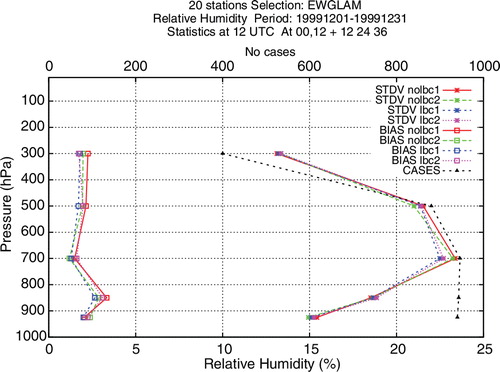
Fig. 10.  BIAS (mean error) and SD (standard deviation of error) verification scores for 500 hPa temperature forecasts over an European domain as verified against radiosonde observations for the forecast lengths +0 h, +12 h, +24 h and +36 h. Verification scores are averaged for the month of December 1999. Experiments nolbc1 (red lines), nolbc2 (green lines), lbc1 (blue lines) and lbc2 (pink lines). Grey line marked CASES shows the number of verifying observations. The EWGLAM (European Working Group on Limited Area Models) list of verifying radiosonde stations is applied.

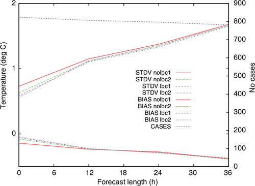
Fig. 11.  BIAS (mean error) and SD (standard deviation of error) verification scores for 500 hPa temperature forecasts over a Scandinavian domain as verified against radiosonde observations for the forecast lengths +0 h, +12 h, +24 h and +36 h. Verification scores are averaged for the month of December 1999. Experiments nolbc1 (red lines), nolbc2 (green lines), lbc1 (blue lines) and lbc2 (pink lines). Grey line marked CASES shows the number of verifying observations.

5.3. Examination of a single forecast case

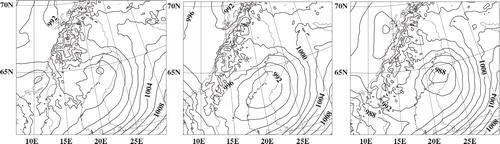
The case providing improved +36 h mean sea level forecasts valid 6 December 1999 12 UTC with control of LBCs was examined in detail. Forecast maps with (method lbc1) and without (method nolbc1) control of LBCs are presented in Fig. 12 together with a verifying analysis (from the experiment with control of lateral boundaries). The control of LBCs results in an improved forecast of the low pressure system over the Bay of Botnia.

Fig. 12.  Mean sea level pressure forecasts 5 December 1999 00UTC + 36 h over a Nordic area without control of lateral boundary conditions (experiment nolbc1, left) and with control of lateral boundary conditions (experiment lbc1, middle). Mean sea level pressure analysis 6 December 1999 12 UTC (experiment lbc1, right). The contour interval is 2 hPa.

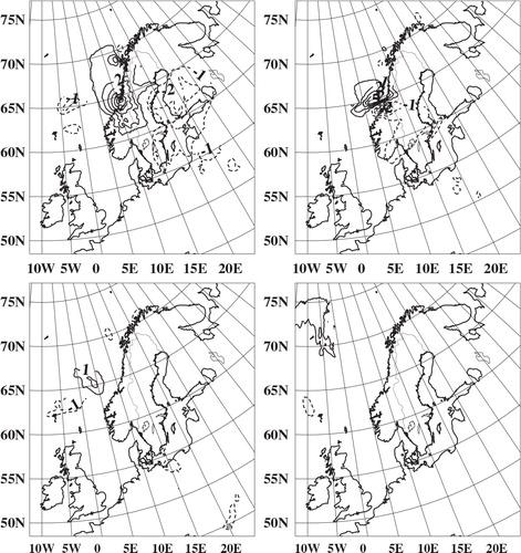
To investigate the origin of the improved forecast based on control of LBCs, difference maps, between forecasts with and without control of LBCs, were produced. The surface pressure forecast differences are shown in Fig. 13 for +36 h, +24 h, +12 h and at analysis time 5 December 1999 00UTC. We may identify a negative-valued surface pressure forecast difference pattern, positioned over Southern Finland and the Bay of Bothnia at +36 h. This forecast difference is associated with the improved forecast using the control of the lateral boundaries. Tracking this forecast difference pattern backwards in time, we may identify a similar negative valued pattern over mid-Sweden at +24 h, over the Norwegian Sea at +12 h and a smaller-scale and smaller amplitude negative valued difference pattern north-west of Scotland, close to the lateral boundary at analysis time. Inspecting also the analysis increment maps for the two assimilation runs, with and without control of lateral boundaries (maps are not shown), one is able to find a much stronger assimilation increment in the middle of the assimilation window for the assimilation run utilising control of LBCs.

Fig. 13.  Differences between surface pressure forecasts, forecasts utilising control of lateral boundary conditions (experiment lbc1) minus forecast not using control of lateral boundary conditions (experiment nolbc1), 5 December 00 UTC +36 h (upper left), +24 h (upper right), +12 h (lower, left) and +00 h (lower, right). The contour interval is 1 hPa.

This forecast difference back-tracking procedure is certainly a bit subjective. To provide some more evidence, we carried out an adjoint model sensitivity experiment (Gustafsson et al., 1998). The differences between one forecast with good verification scores (method lbc1) and one forecast with poor verifications scores (method nolbc1) in a subdomain (60°N–70°N, 5°E–25°E) were taken as the input forecast difference gradients to the adjoint model at 5 December 1999 00 UTC +36 h. The adjoint model was integrated backwards in time until 5 December 1999 00 UTC +00 h to get the sensitivities of these forecast differences with regard to the initial conditions as well as to the LBCs at the initial time. Such an adjoint model integration certainly has limitations as a backtracking tool, in particular the assumption of a tangent linear development, including the application of a very simplified physics package, of forecast perturbations over 36 h may be questioned. The sensitivity patterns are presented for model level 20 (500 hPa) temperature in Fig. 14 (left) for the sensitivity with regard to the initial conditions and in Fig. 14 (right) with regard to the sensitivity to the initial conditions and to the LBCs at the initial time. We can notice that the forecast differences at +36 h according to this procedure are sensitive to initial conditions as well as to LBCs in the area North and Northwest of Scotland.

Fig. 14.  Adjoint model sensitivities of the +36 h forecast differences in Fig. 12 (upper, left) with regard to the initial model level 20 (500 hPa) temperatures (left) and with regard to initial and initial lateral boundary conditions model level 20 temperatures (right). The contour interval is 2 K.

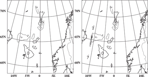
As already described and explained in detail by Gustafsson et al. (1998), the sensitivity patterns with regard to the LBCs have a particular and elongated structure with maximum values in the middle of the lateral boundary relaxation zone, where the gradient of the boundary relaxation weight normal to the lateral boundary has its maximum values.

5.4. Minimisation conditioning and computing cost

The proper formulation and the conditioning of the minimisation problem was one main concern in the design of the control variable for the control of LBCs in this work. The statistical analysis of the time correlation of forecast differences with the NMC method, however, did not support the idea that the original simple formulation by Kawabata et al. (2007), with control of LBCs at the end of the data assimilation window and without any further pre-conditioning, would lead to sub-optimal results and be poorly conditioned. Investigation of the required number of conjugate gradient minimisation iterations over the whole month of December 1999, see Table 1, confirms that this original formulation does not seem to have any problem due to poor conditioning. Introducing the control of the LBCs at the end of the data assimilation window, thus doubling the dimension of the control vector, only adds a few more iterations to obtain the solution to the minimisation. Furthermore, pre-conditioning, by introducing the tendency of the LBCs as the control variable, does not add anything to the efficiency of the minimisation.

Table 1. Average number of conjugate gradient iterations, maximum number of conjugate gradient iterations, average computing time and maximum computing time for 4D-Var minimisations over December 1999

Method	Handling of LBCs	Average number of iterations	Maximum number of iterations	Average time	Maximum time
nolbc1	No control LBCs 0 h = 0	38.5	44	302 s	332 s
nolbc2	No control LBCs 0 h = initial increment	39.1	45	313 s	335 s
lbc1	Control at end of window	40.1	48	325 s	353 s
lbc2	Control of the tendency	40.8	49	356 s	392 s

Two versions of handling the control of lateral boundary conditions and two versions without control of lateral boundary conditions are compared.

We have included also a comparison of the computing time for the 4D-Var minimisation with the two versions of algorithms for controlling the LBCs and for the cases of no control of the LBCs. The computing time refers to using 32 processors on a single computing node of an IBM parallel computer. Controlling the LBCs at the end of the data assimilation window (method lbc1) adds 8% to the computing time for carrying out the 4D-Var data assimilation without the control of the LBCs (method nolbc1). Controlling the tendency of the LBCs (method lbc2) adds another 8% to the computing time. The computing time for the 4D-Var minimisation, without control of LBCs, corresponds roughly to the computing time of a 45-h non-linear forecast model integration. All reported computing times include input and output of all necessary data, as applied in the operational configuration. For a future LAM 4D-Var, with increased non-linear model resolution, with relatively higher resolution in the inner loop minimisation and with a more complete simplified physics package, as compared to the present study, it is likely that the relative increase in computing time due to control of LBCs will remain proportional ().

6. Discussion and concluding remarks

Two versions of algorithms for control of LBCs in the 4D-Var for the HIRLAM forecasting system have been introduced and compared. The first of these algorithms is identical to the algorithm originally proposed by Kawabata et al. (2007) and controls the LBCs at the end of the data assimilation window and it utilises the same statistical information as the background error constraint that is used for the control of the initial conditions. The second algorithm was intended as a pre-conditioning of the first algorithm, and it controls the tendency of the LBCs over the data assimilation window. The second algorithm requires additional statistical information on errors of tendencies of LBCs and these statistics were estimated by the NMC method. Furthermore, during the course of this work it was realised that the LBCs at the start of the data assimilation window can easily be controlled via the control of the initial conditions, consistent with the practice in operational numerical weather prediction to use the initial data as the LBCs at the start of the forecast.

The proposed algorithms for controlling the LBCs were tested and validated in single simulated observation experiments as well as in real observation 4D-Var data assimilation experiments over the whole month of December 1999. A relatively small model domain over the Nordic countries was selected for the real observation experiments in order to maximise the possibilities to show an impact from controlling the LBCs.

The single simulated observation experiments illustrated clearly an improved realism of treating near lateral boundary observations in data assimilation from controlling the LBCs, in particular for the case of strong inflow over the lateral boundaries and with observations simulated at the end of the data assimilation window and downstream from the lateral boundaries. The real observation data assimilation experiments showed a small but positive impact from controlling the LBCs on average forecast verification scores, and it was shown that this positive impact mainly originated from a few isolated situations with a relatively fast propagation of signals from the data assimilation process in the vicinity of the lateral boundary to the centre of the model domain.

The comparison between the two algorithms for controlling the LBCs indicated that the results were comparable, both with regard to the resulting forecast quality and with regard to the conditioning of the minimisation problem. By applying the NMC method to forecast 5-h tendency differences rather than to forecast model state differences, it was possible to show that the algorithm originally proposed by Kawabata et al. (2007) has a good conditioning with regard to the minimisation.

The control of LBCs only requires a modest increase in computing time (8%). Although the impact of the control of the lateral boundaries, as verified by forecast verification scores, turned out to be quite modest, the qualitative evidence provided by the single simulated observation experiments motivates us to recommend the control of LBCs in 4D-Var data assimilation for LAMs.

7. Acknowledgements

I thank the National Center for Atmospheric Research (NCAR) for hosting me and many thanks to Xin Zhang and Xiang-Yu (Hans) Huang for stimulating discussions during my stay at NCAR. I also thank Sigurdur Thorsteinsson and Erland Källén for early contributions to the work reported on here. The contributions of two anonymous reviewers through many useful comments are also acknowledged. Furthermore, Åke Johansson brought a work of Adrian Simmons (2006) to my attention. This work helped me to interpret time correlations of forecast differences. I acknowledge these contributions of Adrian and Åke.

Notes

¹NMC stands for the National Meteorological Center, the former name of NCEP, Washington, USA.

References

- Baxter, G. M, Dance, S. L, Lawless, A. S and Nichols, N. K. 2011. 46, 137–141.
- Berre L. Estimation of synoptic and mesoscale forecast error covariances in a limited-area model. Mon. Wea. Rev. 2000; 128: 644–667.
- Courtier P. Thépaut J.-N. Hollingsworth A. A strategy for operational implementation of 4D-Var, using an incremental approach. Q. J. R. Meteorol. Soc. 1994; 120: 1367–1387.
- Cuxart J. Bougeault P. Redelsperger J. A turbulence scheme allowing for mesoscale and large-eddy simulations. Q. J. R. Meteorol. Soc. 2000; 126: 1–30.
- Dahlgren, P and Gustafsson, N. 2012. Assimilating host model information into a limited area model. Tellus A. 64, 15836. 10.3402/tellusa.v64i0.17518.
- Davies H. C. Limitations of some common lateral boundary schemes used in NWP models. Mon. Wea. Rev. 1983; 111: 1002–1012.
- Errico R. M. Vukićević T. Raeder K. Comparison of initial and lateral boundary condition sensitivity for a limited-area model. Tellus. 1993; 45A: 539–557.
- Gauthier P. Thépaut J.-N. Impact of the digital filter as a weak constraint in the preoperational 4DVAR assimilation system of Météo-France. Mon. Wea. Rev. 2001; 129: 2089–2102.
- Guidard V. Fischer C. Introducing the coupling information in a limited area variational assimilation. Q. J. R. Meteorol. Soc. 2008; 134: 723–735.
- Gustafsson, N. 1992. Use of a digital filter as weak constraint in variational data assimilation. Workshop proceedings on Variational assimilation, with special emphasis on three-dimensional aspects. 327–338. Available from the ECMWF, Shinfield Park, Reading, Berks, RG2 9AX, UK.
- Gustafsson, N, Berre, L, Hörnquist, S, Huang, X.-Y, Lindskog, M and co-authors. 2001. Three-dimensional variational data assimilation for a limited area model. Part I: general formulation and the background error constraint. Tellus. 53A, 425–446.
- Gustafsson, N, Huang, X.-Y, Yang, X, Mogensen, K, Lindskog, M and co-authors. 2012. Four-dimensional variational data assimilation for a limited area model. Tellus A. 64, 14985, DOI: 10.3402/tellusa.v64i0.14985.
- Gustafsson N. Källén E. Thorsteinsson S. Sensitivity of forecast errors to initial and lateral boundary conditions. Tellus. 1998; 50A: 167–185.
- Haugen J.-E. Machenhauer B. A spectral limited-area model formulation with time-dependent boundary conditions applied to the shallow-water equations. Mon. Wea Rev. 1993; 121: 2618–2630.
- Houtekamer P. L. Lefaivre L. Derome J. Ritchie H. Mitchell H. L. A system simulation approach to ensemble prediction. Mon. Wea. Rev. 1996; 124: 1225–1242.
- Janisková M. Theépaut J.-N. Geleyn J.-F. Simplified and regular physical parameterizations for incremental four-dimensional variational assimilation. Mon. Wea. Rev. 1997; 127: 26–45.
- Kain J. The Kain–Fritsch convective parameterization: an update. J. Appl. Meteorol. 2004; 43: 170–181.
- Kawabata, T, Seko, H, Saito, K, Kuroda, T, Tamiya, K and co-authors. 2007. An assimilation and forecasting Experiment of the Nerima Heavy rainfall with a cloud-resolving nonhydrostatic 4-dimensional variational data assimilation system. J. Meteor. Soc. Japan. 85, 255–276.
- Noilhan J. Mahfouf J.-F. The ISBA land surface parameterization scheme. Global Planet Change. 1996; 13: 145–159.
- Parrish D. F. Derber J. C. The National Meteorological Centers spectral statistical interpolation analysis system. Mon. Wea. Rev. 1992; 120: 1747–1763.
- Rasch P. Kristjánsson J. A comparison of the CCM3 model climate using diagnosed and predicted condensate parameterizations. J. Clim. 1998; 11: 1587–1614.
- Savijärvi H. Fast radiation parameterization schemes for mesoscale and short-range forecast models. J. Appl. Meteorol. 1990; 29: 437–447.
- Simmons, A. J. 2006. Observations, assimilation and the improvement of global weather prediction-some results from operational forecasting and ERA-40. In: Predictability of Weather and Climate. T. Palmer and R. Hagedorn. Cambridge University Press: Cambridge, pp. 428–458.
- Trémolet Y. Accounting for an imperfect model in 4D-Var. Q. J. R. Meteorol. Soc. 2006; 132: 2483–2504.
- Undén, P, Rontu, L, Järvinen, H, Lynch, P, Calvo, J and co-authors. 2002. HIRLAM-5 Scientific Documentation. http://www.hirlam.org/.
- Uppala, S. M, Kållberg, P.W, Simmons, A.J, Andrae, U, Da Costa Bechtold, V and co-authors. 2005. The ERA-40 re-analysis. Q. J. R. Meteorol. Soc. 131, 2961–3012.
- Veersé F. Thépaut J.-N. Multiple-truncation incremental approach for four-dimensional variational data assimilation. Q. J. R. Meteorol. Soc. 1998; 124: 1889–1908.