Simulations and scaling of horizontal convection

ABSTRACT

In this paper we describe the results of various numerical simulations of sideways or horizontal convection. Specifically, a two-dimensional Boussinesq fluid is both heated and cooled from its upper surface, but the walls and the bottom of the tank are insulating and have no flux of heat through them. We perform experiments with a range of Rayleigh numbers up to 10¹¹, obtained by systematically reducing the diffusivity. We also explore the effects of a nonlinear equation of state and of a mechanical force imposed on the top surface at a fixed Rayleigh number. We find that, when there is no mechanical forcing, both the energy dissipation and the strength of the circulation itself monotonically fall with decreasing diffusivity. At Rayleigh numbers greater than 10¹⁰ the flow is unsteady; however, the eddying flow is still much weaker than the steady flow at smaller Rayleigh numbers. At high Rayleigh numbers, the stratification and the mean circulation are increasingly confined to a thin layer at the upper surface, with the layer thickness decreasing according to Ra^−1/5. There is no evidence that the flow ever enters a regime that is independent of Rayleigh number. Using a nonlinear equation of state makes little difference to the flow phenomenology at a moderate Rayleigh number. The addition of an imposed stress at the upper surface makes a significant difference in the flow. A strong, energy-dissipating circulation can be maintained even at Ra = 10⁹, and the stratification extends more deeply into the fluid than in the unstressed case. Overall, our results are consistent with the notion that in the absence of mechanical forcing a fluid that is heated and cooled from above cannot maintain a deep stratification or a strong sustained flow at high Rayleigh numbers, even if the interior flow is unsteady.

• horizontal convection
• sideways convection
• meridional overturning circulation
• buoyant plume
• gravity current
• horizontal density gradient

1. Introduction

Ever since the papers of Sandström (1908, 1916), there has been interest, and perhaps some confusion, in the topic of sideways or horizontal convection. On the basis of seemingly general thermodynamic reasoning, Sandström argued that a circulation could only be maintained if the heating in a fluid is at a higher pressure than the cooling so that in hydrostatic fluid the heating must be below the cooling. [Reviews and more discussion are to be found in the studies of Vallis (2006) and Hughes and Griffiths (2008) and references therein.] The implication for the meridional overturning circulation of the ocean is apparent, for here the heating and cooling are at approximately the same level. Nevertheless, the ocean does have a deep overturning circulation, and resolving this paradox has been the subject of many studies since then.

The application of Sandström's ideas to the ocean circulation is not wholly straightforward because he considered a compressible gas whereas the ocean is, to a good approximation, an incompressible Boussinesq liquid. Furthermore Sandström's arguments are heuristic rather than rigorous. However, the Boussinesq nature of the medium in fact makes it possible to put forward arguments that have a firmer foundation. Thus, in a Boussinesq fluid with a linear equation of state, it is easy to show that the heating must be negatively correlated with height in order to maintain a positive energy dissipation in a statistically steady state. Paparella and Young (2002) further showed that, for a Boussinesq fluid that is heated and cooled only at its upper surface, the energy dissipation must go to zero as the diffusivity goes to zero. Specifically, they showed that ɛ < κΔb/H, where ɛ is the energy dissipation, Δb is the maximum buoyancy difference at the surface, H is the depth of the container and κ is the diffusivity of buoyancy. Thus, the flow is ‘non-turbulent’, in the limit (κ, v)→0, with a fixed Prandtl number Pr = v/κ where v is the viscosity, and the energy dissipation vanishes with κ. The essential result has recently been extended by Nycander (2010) and McIntyre (2010) to a nonlinear equation of state, staying in the Boussinesq framework. It should of course be explicitly noted that the surface heat fluxes also go to zero as κ→0, which indicates that the flow will be at rest since the driving force of the system vanishes, and we discuss this point further in Section 4.4. On the other hand, in the limit of infinite Rayleigh number and finite κ, the circulation may of course be non-zero in some dimensional units. Further physical interpretation of the mathematical theory provided by Paparella and Young (2002) can be found in Scotti and White (2011).

None of the mathematical results of the above authors are in any doubt, but they do not address what might be called the phenomenology of the flow. Rossby (1998) had earlier performed some numerical simulations of two-dimensional horizontal convection in a box, forced by a temperature gradient along the bottom surface and with insulating walls and top surface. (There is an up-down symmetry to the problem, so the set-up is equivalent to forcing at the top.) He found that as Rayleigh number increased the strength of the flow increased and the vertical stratification was confined to an increasingly thin layer near the bottom surface. Rossby (1965) also proposed certain scaling relationships for the strength of the flow and its vertical extent, but his simulations (Rossby, 1998) lacked the resolution to properly test them.

In addition to numerical simulations, a number of laboratory experiments of horizontal convection have been performed (see Hughes and Griffiths, 2008, for a summary). These experiments seem to indicate that an interior flow is maintained at high Rayleigh numbers, but their connection to the theoretical and numerical results mentioned above remains unclear (a topic we return to in the last paragraph of Section 6).

If a mechanical forcing is applied to the upper surface of the fluid, thus providing a stress in a similar way to that provided by the wind blowing over the ocean, then the scaling of Rossby (1965) cannot be expected to apply and the mathematical results of Paparella and Young (2002) and their successors do not hold because the stress provides another source of energy to the fluid. It is widely, but not universally, believed that the wind blowing over the ocean in conjunction with tidal forces provides the energy needed to maintain a deep overturning, and a deep stratification, in the ocean (Wunsch and Ferrari, 2004). Consistent with this notion, Whitehead and Wang (2008) performed some laboratory experiments using a rod to provide mechanical mixing extending from top to bottom of the tank. Beardsley and Festa (1972) and Tailleux and Rouleau (2010) found that the addition of mechanical forcing made significant differences to their numerical simulations.

With a goal of clarifying some of the issues raised above we have performed a number of simulations of horizontal convection, going to the highest Rayleigh number that is possible for us. Our objective is to address the following questions:

• In idealised horizontal convection with no mechanical forcing, how does the phenomenology of the flow change as the Rayleigh number increases due to decreasing diffusivity? In particular:

  • Does the scaling of Rossby hold for strength of the circulation and thickness of the thermocline?

  • Does the kinetic energy of the flow, as well as the kinetic energy dissipation, decrease as diffusivity decreases, and if so how?

  • Is the flow steady or unsteady at high Rayleigh number?

  • Is the flow confined to the narrow layer near the surface, or does it feel the depth of the container?

  • Can a deep stratification be maintained at high Rayleigh number?

• Are there qualitative differences in the circulation of fluids with linear and nonlinear equations of state?

• What are the effects of a mechanical stress at the surface?

One motivation of this study is to understand the dynamics of horizontal convection by reducing the diffusivity from eddy diffusion values to the molecular value. This is an important problem for ocean general circulation models where an eddy diffusion is widely used. To this end, we perform idealised numerical simulations of horizontal convection with increasing the Rayleigh number by reducing the diffusivity systematically. We keep the other external parameters (such as buoyancy forcing and geometry) constant and focus on the effects of diffusivity. In non-dimensional terms, the Rayleigh number is increased, but the aspect ratio and Prandtl number are fixed.

This paper is organised as follows: the numerical model and set-up of the numerical experiments are introduced in Section 2. A brief summary about the energetics in the horizontal convection is given in Section 3. The main results are presented in Section 4 for the no-wind case and Section 5 for the case with wind. Finally, we summarise and conclude in Section 6.

2. Model set-up

Our numerical experiments use a two-dimensional (y–z) non-hydrostatic stream function-vorticity model with Boussinesq approximation (Il icak et al., 2008; Il icak and Armi, 2010). With a linear equation of state model equations are then:2.1 2.2 2.3

where б is the vorticity, ψ is the stream function, ν and w are the horizontal and vertical velocities and b is the buoyancy. The density itself is given by where ρ ₀ is the reference density and g is the gravitational acceleration. We discuss the use of a nonlinear equation of state in Section 4.5.

The Jacobian is given by . In the vorticity equation, this is discretised using the Arakawa (1966) scheme to conserve both energy and enstrophy, and eq. (2.1) is then advanced in time using the Adams-Bashforth-3 method. The buoyancy transport eq. (2.2) uses a piecewise parabolic method for advection (Colella and Woodward, 1984), which minimises numerical buoyancy diffusion. The Poisson equation [eq. (2.3)] is solved directly using a Fast Fourier transform, and the entire code is run in parallel. The horizontal and vertical resolution vary depending on the Rayleigh number, with the grid spacing sufficient to resolve the boundary layer at the top with at least 10 grid points at any Rayleigh number. At the highest Rayleigh numbers, we use approximately 1350×1350 grid points in the horizontal and vertical directions.

The computational domain is a rectangular box with a 2:1 (horizontal to vertical) aspect ratio, nominally 20-m long in the y-direction and 10-m deep in the z-direction (although we will describe most results non-dimensionally). Free slip and insulating (no buoyancy flux) boundary conditions are employed for velocity and density fields, respectively, at the left, right and bottom boundaries (i.e. б = 0, ψ=0 and ). We specify the buoyancy and vorticity on the top (z=10 m):2.4 2.5 2.6

where −10 m  <  y < 10 m, A ₀ and ω are the magnitude and frequency of the stress term, respectively. Equation (2.4) provides a plume which potentially continuously provides the abyss with dense fluid. The buoyancy boundary condition is such that the plume forms at the centre of the domain, away from any walls.

The calculations are characterised by three non-dimensional parameters: the Rayleigh number, ; the Prandtl number, ; and the aspect ratio, . We also use a non-dimensional time, , defined by . The Prandtl number is an important parameter in the horizontal convection. Previous studies show that the flow is unsteady and more turbulent in small Prandtl and high Rayleigh numbers (Paparella and Young, 2002; Hughes and Griffiths, 2008). However, in all experiments, we fix the Prandtl number at a value of 10 and the aspect ratio at a value of 1/2 (, ). The buoyancy is only forced by the surface temperature which has a maximum of 15 °C at the top corners and a minimum of 5 °C at the centre with a thermal coefficient of . Thus, the Rayleigh number is equivalently written:2.7

3. Energetics of horizontal convection

In this section, we briefly derive the kinetic and the potential energy equations for later use. To obtain the kinetic energy equation, we multiply eq. (2.1) by −ψ and integrate over the domain (). The Jacobian term vanishes and we obtain:3.1

where , and . The first term on the right-hand side is the conversion from potential energy to kinetic energy (C). The second term on the right-hand side is the viscous dissipation or creating of kinetic energy, D, and after integration by parts and utilisation of either free slip or no-slip lateral boundary conditions it may be written:3.2

where the over bar denotes a horizontal integration. The second term on the right-hand side gives the interior viscous dissipation ɛ. That is, the total interior viscous dissipation of kinetic energy is:3.3

where ɛ is the average dissipation. The first term on the right-hand side of eq. (3.2) is a boundary source of energy due to stress at the surface (the corresponding term involving vanishes because of the lateral boundary conditions). There is a contribution from the top surface when a stress is applied at the top. The boundary energy source term due to the surface stress, , is thus:3.4

The potential energy equation can be derived as follows. Combining the thermodynamic equation [eq. (2.2)] and a kinematic equation for z (i.e. ) gives:3.5

Integrating over the domain, the Jacobian term vanishes and we obtain an equation for the rate of change of potential energy, . That is:3.6

where . The second term on the right-hand side the conversion term, C, described above and the first term is the potential energy production or source term, P. After integrating by parts we obtain:3.7

where . The first term on the right-hand side vanishes because we may choose z=0 at the top and at the bottom so that:3.8

In a statistically steady state with no surface stress, the potential energy creation must equal the kinetic energy dissipation, which immediately leads to the bound obtained by Paparella and Young (2002):3.9

where Δb _max is the maximum difference in buoyancy at the surface. Note that the bound on the total energy dissipation, , is independent of the fluid depth.

If there is a stress on the upper surface (i.e. ) then the energetic balance is:3.10

In this case, there is no obvious useful bound on the interior kinetic energy dissipation.

4. Model results

We first give a qualitative description of the flow, and then investigate the scaling of the thermocline depth and the strength of the circulation change as a function of the Rayleigh number. We then look at the effects of a nonlinear equation of state and the effects of an imposed stress on the top surface. We will use the adjectives ‘low’, ‘moderate’ and ‘high’ to refer to Rayleigh numbers of up to 10⁵, 10⁶–10⁸ and 10⁹ and above, respectively. We focus on experiments with the Rayleigh numbers varying from 10⁶ to 10¹¹ listed in Table 1.

Table 1. Experimental set-up for no-wind cases

	Ra	V (m^2 s^−1)	κ (m^2 s^−1)	A 0 (1 s^−1)	Number of grid points in y, z
NoWind1	10^6	1.2907×10^−2	1.2907×10^−8	0	256×128
NoWind2	10^7	4.082×10^−8	4.082×10^−4	0	256×128
NoWind3	10^8	1.2907×10^−8	1.2907×10^−4	0	512×256
NoWind4	10^9	4.082×10^−4	4.082×10^−5	0	512×256
NoWind5	10^10	1.2907×10^−4	1.2907×10^−5	0	800×512
NoWind6	10^11	4.082×10^−5	4.082×10^−6	0	1350×1350

4.1. A descriptive overview of experiments with no stress

The simulations are typically begun with the fluid at rest and at a uniform temperature slightly warmer than the lowest temperature to be applied, at the surface. As soon as the upper boundary conditions are applied, a fast-growing plume develops from the top surface. This plume reaches the bottom and drives an energetic circulation that is dependent on the geometry of the tank, forcing, dissipation and initial state of the flow. Eventually, the flow settles down into a steady state, or at least a statistically steady state. We integrate forward until three criteria are satisfied. First, the net heat flux into the fluid must be negligible. Second, the energetic terms must be in balance when integrated over the box. Third, the integration should be for at least as long as a diffusion time scale, , where H is the tank height. In practice, this is by far the most severe criterion and after integrations of this length, all the budgets are well balanced, and the flow is manifest in a steady state or statistically steady state. 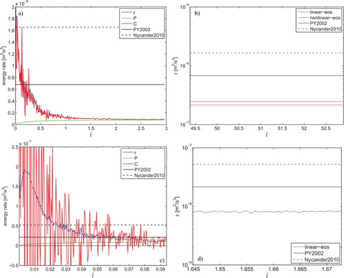In dimensional terms, we need to integrate 0.9, 2.8, 8.9, 28.4 and 89.7 d for the simulations of the Rayleigh numbers 10⁶, 10⁷, 10⁸, 10⁹ and , respectively. For the low Rayleigh numbers, we integrated the numerical model for 15 computational days, while moderate and high Rayleigh number experiments needed approximately 150 d. The highest Rayleigh number experiment Ra = 10¹¹ is started from final state of the Ra = 10¹⁰ experiment. A typical evolution of the terms in the energy budget is shown in Fig. 1, with the generation, conversion and dissipation terms eventually coming into a good balance.

Fig. 1.  Energetics at Ra = 10⁷ (top) and Ra = 10¹⁰ (bottom). Specifically, (a) evolution of the energy budget at Ra = 10⁷ with linear equation of state. At the later stages of the integration, the kinetic energy dissipation, ɛ, is equal to the conversion of potential energy to kinetic energy (C) which in turn is equal to the generation of potential energy by the thermodynamic forcing, P. (b) ɛ versus time for experiments with different equations of state at Ra = 10⁷, and the upper bounds established by Paparella and Young (2002) and Nycander (2010). (c) Same as (a) but at Ra = 10¹⁰. (d) Same as (b) but only for linear equation of state. In all panels, the time is scaled by the diffusion time, H ²/κ where H is the total depth of the domain and κ is the diffusivity used in the experiment.

At the low Rayleigh numbers (Ra = 10³–10⁵) the flow evolves into a steady, strong and deep circulation extending throughout the domain, similar to the circulation previously found by Rossby (1998). As the Rayleigh number increases, the circulation becomes shallower and the stratification becomes confined to a shallow layer near the surface, generally consistent with the simulations of Rossby (1998), Paparella and Young (2002) and Siggers et al. (2004). (This boundary layer might be regarded as an analogue of the diffusive component of the oceanic thermocline, with a thickness decreasing as the Rayleigh number increases.) At low and moderate Rayleigh number the flow is very nearly absolutely steady, becoming shallower as the Rayleigh number decreases. Indeed, at moderate Rayleigh number the flow appears to be essentially independent of the depth of vessel. The fluid below the top boundary layer is virtually unstratified, and the deep fluid is almost at rest.

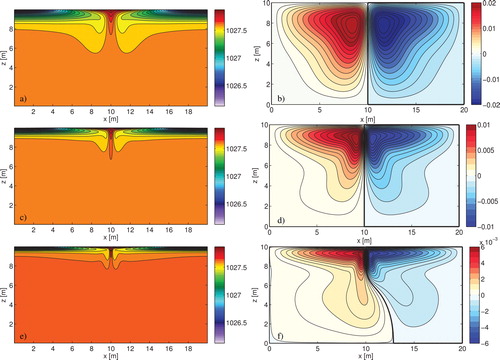
Figure 2 shows time-averaged stream function and density fields for Ra = 10⁶, 10⁷ and 10⁸. It can be clearly seen that there is a sinking region in the middle of the tank and a broad upwelling for the rest of the domain. One of the most important features is that the strength of the circulation decreases as the Rayleigh number increases (see colour bar of Fig. 2a, c and e). At higher Rayleigh number the centre of the convection cell is concentrated very close to the centre of the tank, and a boundary layer is established. Both density and stream function fields reveal that the circulation moves to the top and the thermocline thickness decreases as the Rayleigh number is increased (Fig. 2b, d, and f). It is also clearly seen that the density in the interior of the tank is nearly uniform. For the low and moderate Rayleigh numbers, these results are consistent with the previous studies (Rossby, 1998; Paparella and Young, 2002).

Fig. 2.  Time-averaged density field contours (left column) for and stream function (right column) for: (a) and (b) Ra = 10⁶; (c) and (d) Ra = 10⁷, (e) and (f) Ra = 10⁸. At these Rayleigh numbers, the flow is almost steady, and snapshots are very similar.

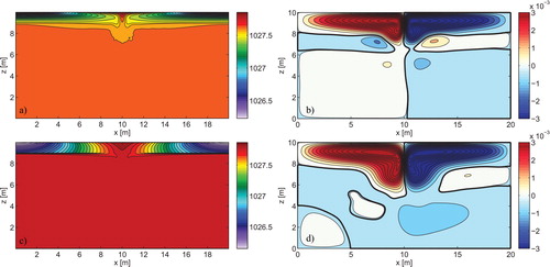
At high Rayleigh number the circulation is increasingly confined to the top of the tank (Fig. 3), with the strength of the circulation and the thermocline thickness decreasing as the Rayleigh number increases. The time-averaged flow does not feel the bottom of tank at Rayleigh numbers of 10⁹ and above, and the thermocline becomes very thin. At Rayleigh numbers of 10⁹ and lower, the flow is almost absolutely steady, but as the Rayleigh number is further increased to 10¹⁰ and higher, the flow becomes unsteady, seemingly because of a fluid dynamic instability in the descending plume, and eddying flow fills the domain (Fig. 4). However, the unsteady flow is weak, and its kinetic energy is less than that of the flow at lower Rayleigh numbers. Furthermore, the stratification remains confined to an extremely thin boundary layer near the upper surface, and the deeper eddying flow takes place in an essentially unstratified fluid. The flow is even more unsteady at Ra = 10¹¹, although we have not integrated that experiment for a full diffusion time.

Fig. 3.  As for Fig. 2, but for Rayleigh numbers of, from the top: Ra = 10⁹, Ra = 10¹⁰, and Ra = 10¹¹. At Ra = 10¹⁰ and Ra = 10¹¹, the flow is unsteady.

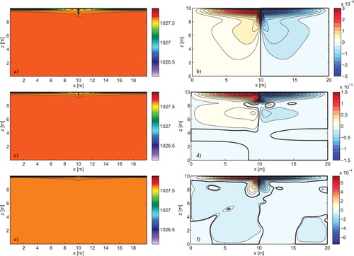
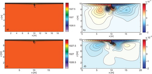
Fig. 4.  Snapshots of the density (left) and the stream function (right) fields of the Ra = 10¹⁰ experiment.

4.2. Scaling for the no-stress experiments

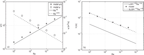
We now test certain scaling arguments for different Rayleigh number experiments and, in the following subsection, the degree to which various energetic inequalities are satisfied. Rossby (1965) suggested that the stream function and thermocline depth in the horizontal convection are the functions of the Prandtl and Rayleigh numbers, specifically that:4.1

and4.2

where the hats denote non-dimensional values. For a fixed Prandtl number, eq. (4.1) implies that the dimensional stream function varies as Ra^−3/10 since Ra is increased by reducing the diffusivity.

Dimensional and non-dimensional maximum stream function of the mean flow is plotted as a function of the Rayleigh number shown in Fig. 5a. There is generally a good agreement between the model results and suggested scalings (black line in Fig. 5a) for the stream function. The thermocline depth as a function of the Rayleigh number is shown in Fig. 5b. The model results are also in good agreement with the theoretical scaling, (dashed line in Fig. 5b). The thermocline depth decreases monotonically as the Rayleigh number is increased. Neither the circulation strength nor the thermocline thickness shows any indication of asymptoting to a value independent of the Rayleigh number in any of the experiments we have performed.

Fig. 5.  (a) Non-dimensional stream function () and dimensional stream function versus Rayleigh number, (b) Thermocline depth (h) versus Rayleigh number for no-wind experiments.

As shown in Fig. 6a, we plot both total kinetic energy and the kinetic energy of the time mean flow as a function of the Rayleigh number (the total kinetic energy is the time average of the kinetic energy, including the eddying flow). For Rayleigh numbers of 10⁹ and below the flow is steady, but is increasingly unsteady at higher Rayleigh number. Nevertheless, the kinetic energy of the eddying flow continues to decrease with increasing Rayleigh number. The eddying flow kinetic energy as a function of time is shown in Fig. 6c for the Ra = 10⁹, Ra = 10¹⁰ and Ra = 10¹¹ cases. Note that, although there is an unsteady eddying flow for the high Rayleigh numbers, the stratification is confined to the very shallow upper cell, and there is very little buoyancy injection into the interior, which remains almost totally unstratified. The Reynolds number also increases monotonically, albeit slowly, with the Rayleigh number. Defining the Reynolds number as where , then in Fig. 6b we see that as the Reynolds number increases approximately as the one-quarter power of the Rayleigh number.

Fig. 6.  (a) The total kinetic energy of the flow for various values of the Rayleigh number is increased. Circles are the kinetic energy of the time-mean flow, and stars are the time-averaged kinetic energy of the total flow, including eddying terms. (b) Reynolds number, , as a function of Rayleigh number. (c) Total kinetic energy as a function of time for the Ra = 10⁹, 10¹⁰ and 10¹¹ cases. Time is scaled by the diffusion time, H ²/κ with κ the diffusivity at Ra = 10¹⁰.

4.3. Energy and buoyancy variance dissipation

The bound on the kinetic energy dissipation rate can be written as:4.3

That is, if the diffusivity is varied, the bound varies linearly with the diffusivity itself and with the inverse half power of the Rayleigh and Prandtl numbers.

Figure 7 shows the energy dissipation rate as a function of the Rayleigh number in our experiments with varying diffusivity, a linear equation of state and no wind. The model results are smaller than the bound in all cases (as they should be), and in fact scales in a similar fashion as theoretical bound. There is no indication of any anomalous scaling up to Rayleigh numbers of 10¹¹.

Fig. 7.  (a) Mean dissipation rate (ɛ) and non-dimensional dissipation rate () versus Rayleigh number. (b) Buoyancy variance dissipation rate (χ) as a function of diffusivity, κ.

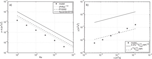
Another bound for the horizontal convection is the upper limit of the variance dissipation rate () provided by Siggers et al. (2004) and Winters and Young (2009). They show that χ is bounded from above by:4.4

Thus, χ should diminish at least as fast as κ ^1/3 in the limit κ→ at the fixed Prandtl number. Our results are shown in Fig. 7b. The model results for χ are considerably lower than the theoretical upper bound. However, the buoyancy variance decreases with κ ^3/5 rather than κ ^1/3.

4.4. Effect of increased diffusion near surface

We have shown that in the case of a uniform and small diffusivity, the circulation is confined to the top, and the strength of the circulation decreases with diffusivity. However, in the real ocean there is a turbulent mixed layer homogenised by the wind stress. In this mixed layer, the effective diffusivity values are approximately two orders of magnitude higher than the background value and the buoyancy fluxes into the ocean are large, even though the molecular diffusivity is small.

To emulate this mixed layer, we have performed two additional simulations with non-uniform diffusivities. In the first experiment, the dimensional diffusivity value at the top 10% of the tank is κ=4.082×10⁻⁴ and the diffusivity at the rest of the tank is κ=4.082×10⁻⁵ m² s⁻¹. For the second experiment, we increased the diffusivity to 4.082×10⁻³ m² s⁻¹ at the top 10% of the tank. In both cases, the enhanced diffusivity covers a depth larger than the Rossby depth with the small diffusivity, but less than the Rossby depth with the large diffusivity. These changes allow, in principle, substantial surface fluxes. Our goal is not to explore parameter space fully; rather, it is to see if these changes lead to qualitative changes in the deep circulation.

Time-averaged density fields are shown in Fig. 8a and c. Evidently, the stratification at the top of the tank is increased in both the cases, and the increased density gradient at the top leads to larger available potential energy (APE) in the system. This additional energy does drive a stronger and somewhat deeper circulation (Fig. 8b and d) compared with the uniform diffusivity case (Fig. 3d). However, even though the vertical extent of the circulation increases, it still does not penetrate to bottom of the tank. Of course, there remains the possibility that if we use a still larger diffusivity at the top, there might be enough energy and vertical velocity pumping to drive a deeper circulation. A more complete exploration of this phenomena is called for, but this is beyond the scope of the present work.

Fig. 8.  (a) Time-averaged density field contours (left column) for and stream function (right column) for: (a) and (b) at the top and at the bottom of the tank; (c) and (d) at the top and at the bottom of the tank.

4.5. Effect of equation of state

The Boussinesq equations are not limited to a linear equation of state. More generally, the buoyancy equation [eq. (2.2)] may be replaced by a thermodynamic equation of the form:4.5a 4.5b

where θ and S are semi-conservative tracers and eq. (4.5b) is an equation of state. If the equation of state is of the above form, and specifically is a function of z and not pressure, then the adiabatic versions of these equations [with ] properly conserve an energy (or a dynamic enthalpy) and, in the absence of salinity, potential vorticity (Vallis, 2006; Young, 2010).

Nycander (2010) and McIntyre (2010) generalised the non-turbulence results of Paparella and Young (2002) to the nonlinear equation state given by Vallis (2006), namely:4.6

where c _s is the speed of sound. The terms proportional to γ and describe the thermobaric effect and cabelling, respectively. The above equation reduces to the linear equation of state if γ, and β _s are set to zero, and the sound speed set to infinity. Nycander (2010) showed that when the nonlinear equation state is employed, the dissipation of kinetic energy is still bounded by the diffusivity according to:4.7

where .

To explore whether the flow phenomenology is affected by a nonlinear equation of state, we perform integration with a nonlinear equation of state using the Rayleigh number equal to 10⁷ (i.e.  m² s⁻¹ in the dimensional configuration). We rescale the z-dependence in eq. (4.6) with the depth of the tank, so that the density variation due to depth is similar to that of a 5000-m deep ocean, and set β _s=0 so that salinity has no effect. There is also no wind forcing in these experiments. Figure 1a shows the initial evolution of the energetic terms, defined in Section 3, for the experiment with the linear equation of state.

After the flow has equilibrated, the energy budget is balanced. Furthermore, the dissipation rate is always under the theoretical upper bounds, as is expected. Fig. 1b shows the dissipation term (ɛ) for the experiment with linear and nonlinear equations of state after the flow is reached a steady state. It can be seen that dissipation rates are very close to each other in both experiments. Similarly, the steady-state stream function and density fields for the two experiments are shown in Fig. 9. There is a strong circulation at the middle-upper side of the domain for both experiments (Fig. 9a and c). As we expected, both circulations are similar to each other in terms of magnitude and vertical/horizontal structure. The thermocline is visible for the linear equation of state experiment (Fig. 9b). On the other hand, the flow is linearly stratified in Fig. 9d, but solely because of the effect of nonlinear equation of state. Overall, we conclude that the effect of nonlinear equation of state is small, at least for moderate Rayleigh numbers, and we have no reason to suppose that this result does hold at high Rayleigh number. For this reason, we did not explore the effects of a nonlinear equation of state further.

Fig. 9.  Time-averaged stream function fields at Ra = 10⁷ for (a) linear equation of state, (c) nonlinear equation of state. Time-averaged density fields at Ra = 10⁷ for (b) linear equation of state, (d) nonlinear equation of state.

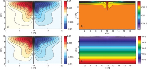
Table 2. Experimental set-up for wind cases

	Ra	A 0 (1 s^−1)	ω (1 s^−1)
Wind1	10^9	0.0256	N 0=0.04
Wind2	10^9	0.0256	5N 0=0.2
Wind3	10^9	0.0256	N 0/5 = 0.008
Wind4	10^9	0.16	N 0=0.04
Wind5	10^9	0.16	5N 0=0.2
Wind6	10^9	0.16	N 0/5 = 0.008
Wind7	10^9	0.432	N 0=0.04
Wind8	10^9	0.432	5N 0=0.2
Wind9	10^9	0.432	N 0/5 = 0.008
Wind10	10^9	1.0	N 0=0.04
Wind11	10^9	1.0	5N 0=0.2
Wind12	10^9	1.0	N 0/5 = 0.008

5. Experiments with an imposed stress

We now investigate the effects of imposing a stress on the top surface, roughly mimicking the effects of wind on the ocean. We do this by applying a non-zero surface boundary condition for the vorticity field, as in eq. (2.5). The forcing is periodic in order not to simply impose a mean flow on the system. The parameters of the forcing are the amplitude, A ₀ and the frequency, ω. We perform all experiments at Ra = 10⁹. One of the natural frequencies in the problem is the buoyancy frequency, N, which in turn is related to the surface forcing, and a natural scaling for the amplitude is the surface vorticity in the absence of wind forcing, which we denote . With this in mind, we perform experiments at three different frequencies: (1) , where Δb is the difference in the imposed buoyancy across the top surface; (2) and (3) . For each frequency we use four different values that are chosen for A ₀ as the wind forcing magnitude: (1) which is the maximum vorticity value in the steady-state no-wind simulation; (2) which is considered as a strong forcing; (3) which is considered a weak forcing (Table 2). For most experiments the stress is applied uniformly over the entire upper surface. We have also performed experiments in which the stress is varying sinusoidally, that is with , but the results do not change our conclusions.

In the cases with the weakest forcing (), there are no significant changes compared to the no-stress case, although the depth to which the stream function penetrates, and the thermocline thickness, increases somewhat. On increasing the magnitude of the vorticity at the surface to , the circulation becomes significantly deeper for the and (Fig. 10b and d). However, the high-frequency experiment () is similar to the no-wind case, suggesting that the wind forcing does not have enough time to penetrate downwards, and the induced positive and negative values in the vorticity field effectively cancel each other.

Fig. 10.  Time-averaged density field contours for (a) A ₀=0.16, ω=0.008; (c) A ₀=0.16, ω=0.04 and (e) A ₀=0.16, ω=0.2. Time-averaged stream function contours for (b) A ₀=0.16, ω=0.008; (d) A ₀=0.16, ω=0.04 and (f) A ₀=0.16, ω=0.2.

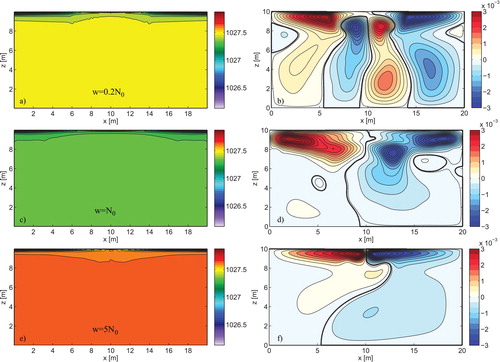
The fourth magnitude of A ₀ is equal to 0.433 which is approximately . The effect of the magnitude of the surface vorticity becomes still more significant when we increase to strength of the forcing to A ₀=2.6б ₀. There are now strong deep reaching circulations for both the ω=N ₀ and ω=N ₀/5 (Fig. 11b and d), and the magnitude of the stream function is typically larger than the maximum stream function in the no-wind case. The dense water is sinking from the side walls instead of the middle of the tank because the surface waters are pushed to the side boundaries where they are forced to sink. The water that does sink to the bottom of the tank is no longer as cold as in the no-stress case because it has insufficient time to take on the temperature at the surface at the side walls. Thus, the overall stratification (i.e. top to bottom temperature difference) is generally smaller in the stressed case, although the main thermocline, away from the main plumes, is a little deeper (see Fig. 12 for an example). On the other hand, the circulation for the high-frequency (ω=5N ₀) experiment does not reach bottom unlike the other two experiments (Fig. 11f).

Fig. 11.  Time-averaged density field contours for (a) A ₀=0.4213, ω=0.008; (c) A ₀=0.4213, ω=0.04 and (e) A ₀=0.4213, ω=0.2. Time-averaged stream function contours for (b) A ₀=0.4213, ω=0.008; (d) A ₀=0.4213, ω=0.04 and (f) A ₀=0.4213, ω=0.2.

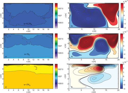
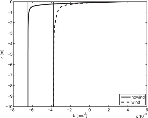
Fig. 12.  Spatial and time-averaged buoyancy profile for the no-wind case (solid line) and wind case (dashed line) with A ₀=0.16 and ω=N ₀, away from the sinking region. The straight vertical lines are the values at the bottom of the domain.

Finally, we compute the kinetic energy dissipation, the buoyancy variance dissipation and the maximum stream function. The kinetic energy dissipation rate is shown in Fig. 13a for all cases with the wind forcing. The green star and green circles display the dissipation rate in the no-wind model result and the theoretical upper limit ɛ corresponds to Ra = 10⁹, respectively. Increasing the amplitude of the boundary value of vorticity (A ₀) increases the dissipation rate and allows the dissipation rates to be larger than the theoretical limit in the unstressed case. In all the wind experiments, the high frequency of the wind forcing leads to smaller dissipation rates (black stars in Fig. 13a), and this is because the flow does not have enough time to adjust to the forcing and the forced circulation is weak. The dissipation rates for the experiments with the natural buoyancy frequency (ω=N ₀) at A ₀=б₀/6 and A ₀=б₀ are larger than the ones with smaller frequency ω=N ₀/5. The latter becomes larger than the former for amplitudes of A ₀=2.5б₀ and A ₀=6б₀.

Fig. 13.  (a) Mean dissipation rate (ɛ) versus strength of the wind. (b) Buoyancy variance dissipation rate (χ) as a function of strength of the wind. (c) Maximum stream function versus strength of the wind.

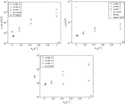
The buoyancy variance dissipation rates are shown in Fig. 13b and results are similar to those for kinetic energy dissipation rate. The green star dot is the control case with no-wind forcing. The green diamond and circles are approximate buoyancy variance () and the theoretical upper limit (), respectively. The buoyancy variance dissipation in the high-frequency forcing is lower than the other two frequency model results. Similar to the momentum dissipation rate, the buoyancy dissipation rate is the largest in simulations with ω=N ₀ at A ₀=б₀/6 and A ₀=б₀ and simulations with ω=N ₀/5 at A ₀=2.5б₀ and A ₀=6б₀. Although increase in A ₀ leads to increase in χ, all buoyancy variance dissipation rates of wind experiments are, in fact, still below the theoretical upper limit described by Winters and Young (2009). Figure 13c shows the maximum non-dimensional stream function, , as a function of strength of the surface vorticity. The maximum stream function values are always higher than the one in the no-wind case, and the strength of the circulation increases with larger surface vorticity values.

Tailleux and Rouleau (2010) suggest that APE may be a useful diagnostic, as APE production is directly proportional to the strength of the overturning. They show that mechanical stirring due to winds results in more diapycnal mixing, higher APE and increased the strength of the circulation. Motivated by their work, the APE values for different cases are shown in Fig. 14. When we decrease the diffusivity in the no-wind experiments, the thermocline depth decreases and is increasingly confined to the top of the tank, and this leads to a decrease in the APE as shown in Fig. 14a. That is, as diffusivity decreases with zero mechanical forcing so does the APE, and the deep circulation diminishes. Consistently, both the APE and the circulation strength can be increased by stronger buoyancy forcing − that is, by imposing a larger temperature gradient at the surface leads. On the other hand, the experiments with a surface stress show that the APE increases with the strength of the wind. Warm water is pushed to the bottom of the tank and a deeper thermocline depth in the stressed experiments. This can be clearly seen in the buoyancy profiles in Fig. 12.

Fig. 14.  (a) Available potential energy as a function of diffusivity, κ. (b) Available potential energy versus strength of the wind.

6. Summary and conclusions

We have performed a variety of numerical simulations of a Boussinesq fluid heated and cooled from above. We performed experiments over a range of Rayleigh numbers up to 10¹¹, by decreasing diffusivity, with a linear and nonlinear equation of state, and looked at the effects of imposing a mechanical stress at the upper surface, somewhat akin to wind forcing on the ocean. The conclusions of this study are itemised below. Note that they strictly apply only to a two-dimensional Boussinesq fluid in which heating and cooling are applied at the top surface by way of a Dirichlet boundary condition on buoyancy:

• With a linear equation of state the strength of the circulation monotonically decreases as the diffusivity decreases at fixed Prandtl number (here equal to 10). There is no evidence that the flow ever becomes independent of the Rayleigh number.

• At Rayleigh numbers up to 10⁹ the equilibrated flow is steady. At higher Rayleigh numbers the flow is unstable, with eddying flow filling the domain. However, the total kinetic energy (eddies plus mean flow) and the kinetic energy dissipation still decrease with decreasing diffusivity. Additional integrations with different numerical schemes and at different Prandtl numbers would be needed to understand the robustness of lack of steadiness, and it does not affect our other conclusions.

• As the Rayleigh number increases, the stratification and the time mean flow become increasingly confined to a shallow layer near the surface, independent of the depth of the tank. Even when the flow is unsteady, the stratification is virtually all confined to a shallow layer, as is the mean circulation. The deep eddying circulation that arises at high Rayleigh number takes in an unstratified region of fluid.

• The depth of the stratified layer appears to vary as Ra^−1/5 to a good approximation, as first suggested by Rossby (1965).

• The buoyancy variance dissipation rate decreases with decreasing diffusivity (κ), and is well below the bounds of Winters and Young (2009).

• The inclusion of a nonlinear equation of state makes no substantial difference to the flow structures at a Rayleigh number up to 10⁷.

• The addition of a mechanical stress at the top surface makes a substantial, qualitative difference to the structure of the flow and to the stratification. Specifically, (1) the stratification extends further into the interior at small diffusivity; (2) a deep eddying flow can be maintained, the strength of which increases with the strength of the mechanical forcing, and which is sensitive to the frequency of the forcing.

What do these results imply about fluids more generally and about the circulation of the ocean? First, they are generally consistent with what might be known as Sandström's effect (we prefer not to call it Sandström's theorem). That is to say, as the diffusivity becomes smaller and smaller in a fluid heated and cooled from above, the strength of the interior flow diminishes (even if it is unsteady) and the stratification is confined to an ever thinner layer at the upper surface. As demanded by the result of Paparella and Young (2002) the kinetic energy dissipation is bounded by κ, and our numerical results also show that the kinetic energy itself and the deep stratification also both diminish as the diffusivity diminishes. There is no sustained deep mean flow at high Rayleigh number, although there may be a continuing, albeit weak, eddying flow at high Rayleigh number.

It should be noted that we increase the Rayleigh number by decreasing the diffusivity and keep other parameters fixed. One motivation for this is to better understand the phenomenology of horizontal convection as we change the diffusivity from eddy diffusion values to the molecular value. This approach has two implications: (1) as the diffusion decreases so do the dimensional surface fluxes, thus there will be less APE in the system; (2) the system's energy dissipation depends on diffusivity, thus smaller diffusion values lead to less dissipation and, if the scales of the motion stay the same, a weaker circulation. If we were to increase the Rayleigh number by increasing the buoyancy forcing the dimensional stream function would increase, as we would the APE and total dissipation in the system. Of course, although the dimensional results depend on many physical parameters, the non-dimensional results from which all dimensional results can be derived depend on only three non-dimensional numbers (Rayleigh, Prandtl and aspect ratio).

The addition of a mechanical stress at the surface makes a significant difference. It enables the stratification to extend further into the fluid interior, deepening the thermocline, and allows the mean flow to cross the stratification. It is as if the mechanical forcing allows there to be an ‘eddy diffusivity’, although given the unrealistic nature of the imposed stress vis-à-vis the wind over the real ocean we should not draw too strong an analogy between our simulations and the wind-forced ocean. The addition of an enhanced diffusivity at the top of the domain also makes a difference to the circulation, but we note that such an enhanced diffusivity would, in the real ocean, have its origins in wind forcing. The effects of nonlinearity in the equation of state are small in the experiments we have performed, and although we cannot be definitive it seems very unlikely that nonlinearities in the equation of state, or the fact that seawater is not exactly Boussinesq, can make a significant impact on the real ocean vis-a-vis the relevance of horizontal convection.

If we were to take the speculative step of extrapolating our results to the real ocean, we would conclude that the effects of mechanical forcing (i.e. winds and tides) are crucial to the maintenance of a deep stratification and to a mean flow beneath the main thermocline. It may be that we can still usefully think of the deep flow as being maintained by the combined effects of buoyancy and mixing, as in the classical picture, provided that we remember that the mixing – the ‘eddy diffusivity’ – has its origins in the wind and tides, as noted by Vallis (2006) and by Tailleux and Rouleau (2010).

In spite of the seemingly unambiguous nature of our numerical results, we do need to point out that various experimental results (Hughes and Griffiths, 2008) and others performed at the Australian National University in Canberra (K. Stewart, A. Hogg, personal communication) appear to tell a different story. The experiments seem to indicate that a vigorous deep circulation can be maintained in a fluid, with buoyancy forcing only at the surface, in apparent contradiction with the numerical results we have presented. There are many possible reconciliations of the two classes of results, of which the following seems most likely to us. (1) The two-dimensional nature of the numerical experiments might give a misleading picture of what happens in a real fluid. (2) The experimental results have not reached a true equilibrium. (3) The surface fluxes in the experimental results are not small, even with small diffusivity, and this enables a deep circulation to be maintained. (4) There would be no real contradiction, if the experimental results and numerical results could be quantitatively compared. Exploring these possibilities is an important future task.

Acknowledgements

We thank Andy Hogg for suggesting the experiment with enhanced diffusion near the surface and the anonymous reviewers for their comments. This work was supported by NSF award OCE-1027603 and DOE award DE-SC0005189.

References

- Arakawa A. Computational design for long-term numerical integration of the equations of fluid motion: two dimensional incompressible flow. Part I. J. Comput. Phys. 1966; 1: 119–143. 10.3402/tellusa.v64i0.18377.
- Beardsley R. C. Festa J. F. A numerical model of convection driven by a surface stress and non-uniform horizontal heating. J. Phys. Oceanogr. 1972; 2: 444–455.
- Colella P. Woodward P. R. The piecewise parabolic method (PPM) for gas-dynamical simulations. J. Comput. Phys. 1984; 54: 174–201. 10.3402/tellusa.v64i0.18377.
- Hughes G. O. Griffiths R. W. Horizontal convection. Ann. Rev. Fluid Mech. 2008; 40: 185–208. 10.3402/tellusa.v64i0.18377.
- Il icak M. Armi L. Comparison between a non-hydrostatic numerical model and analytic theory for the two-layer exchange flows. Ocean Model. 2010; 35: 264–269. 10.3402/tellusa.v64i0.18377.
- Il icak M. Özgökmen T. M. Peters H. Baumert H. Z. Iskandarini M. Very large eddy simulation of the Red Sea overflow. Ocean Model. 2008; 20: 183–206. 10.3402/tellusa.v64i0.18377.
- McIntyre, M. E. 2010. On spontaneous imbalance and ocean turbulence: generalizations of the Paparella–Young epsilon theorem. In: Turbulence in the Atmosphere and Oceans. D. G. Dritschel). Proceedings of International IUTAM/Newton Institute Workshop, 8–12 December. Heidelberg, Springer, 3–15.
- Nycander J. Horizontal convection with a non-linear equation of state: generalization of a theorem of Paparella and Young. Tellus A. 2010; 62: 134–137. 10.3402/tellusa.v64i0.18377.
- Paparella F. Young W. R. Horizontal convection is non-turbulent. J. Fluid Mech. 2002; 466: 205–214. 10.3402/tellusa.v64i0.18377.
- Rossby T. On thermal convection driven by non-uniform heating from below: an experimental study. Deep-Sea Res. 1965; 12: 9–16.
- Rossby T. Numerical experiments with a fluid heated non-uniformly from below. Tellus A. 1998; 50: 242–257. 10.3402/tellusa.v64i0.18377.
- Sandström J. W. Dynamische versuche mit meerwasser. Ann. Hydrodynam. Mar. Meteorol. 1908; 36: 6–23.
- Sandström J. W. Meteorologische studien im schwedischen hochgebirge. Göteborgs Kungl. Vet. Handl. 1916; 17: 4–48.
- Scotti A. White B. Is horizontal convection really non-turbulent?. Geophys. Res. Lett. 2011; 38: 21609.10.3402/tellusa.v64i0.18377.
- Siggers J. H. Kerswell R. R. Balmforth N. J. Bounds on horizontal convection. J. Fluid Mech. 2004; 517: 55–70. 10.3402/tellusa.v64i0.18377.
- Tailleux R. Rouleau L. The effect of mechanical stirring on horizontal convection. Tellus. 2010; 62A: 138–153.
- Vallis G. K. Atmospheric and Oceanic Fluid Dynamics. Cambridge University Press: Cambridge, 2006
- Whitehead J. A. Wang W. A laboratory model of vertical ocean circulation driven by mixing. J. Phys. Oceanogr. 2008; 38: 1091–1106. 10.3402/tellusa.v64i0.18377.
- Winters K. B. Young W. R. Available potential energy and buoyancy variance in horizontal convection. J. Fluid Mech. 2009; 629: 221–230. 10.3402/tellusa.v64i0.18377.
- Wunsch C. Ferrari R. Vertical mixing, energy, and the general circulation of the oceans. Ann. Rev. Fluid Mech. 2004; 36: 281–314. 10.3402/tellusa.v64i0.18377.
- Young W. R. Dynamic enthalpy, conservative temperature, and the seawater Boussinesq approximation. J. Phys. Oceanogr. 2010; 40: 394–400. 10.3402/tellusa.v64i0.18377.