A hybrid nudging-ensemble Kalman filter approach to data assimilation. Part II: application in a shallow-water model

ABSTRACT

A hybrid nudging-ensemble Kalman filter (HNEnKF) data assimilation approach, explored in the Lorenz three-variable system in Part I, is tested in a two-dimensional shallow-water model for dynamic analysis and numerical weather prediction. The HNEnKF effectively combines the advantages of the ensemble Kalman filter (EnKF) and the observation nudging to achieve more gradual and continuous data assimilation by computing the nudging coefficients from the flow-dependent, time-varying error covariances of the EnKF. It can also transform the gain matrix of the EnKF into additional terms in the model's predictive equations to assist the data assimilation process. The HNEnKF is tested for both a wave case and a vortex case with different observation frequencies and observation networks. The HNEnKF generally produces smaller root mean square (RMS) errors than either nudging or EnKF alone. It also has better temporal smoothness than the EnKF and lagged ensemble Kalman smoother (EnKS). The HNEnKF allows the gain matrix of the EnKF to be applied gradually in time, reducing the error spikes commonly found around the analysis times when using intermittent data assimilation methods. Therefore, the HNEnKF produces a seamless analysis with better inter-variable consistency and dynamic balance than the intermittent EnKF.

• ensemble Kalman filter (EnKF)
• nudging
• hybrid data assimilation
• dynamic balance
• insertion noise
• shallow-water model

1. Introduction

Data assimilation is critical for providing the best possible analysis and improving model forecasts. The ensemble Kalman filter (EnKF), first proposed by Evensen (1994), has become a popular data assimilation method for atmospheric applications (e.g. Houtekamer and Mitchell, 1998; Anderson, 2001; Whitaker and Hamill, 2002), where it is able to provide a flow-dependent estimate of the background error covariances used to determine the weights of the observations within a data-assimilation analysis. However, the EnKF, an intermittent data assimilation scheme, performs a data-assimilation analysis at each observation time and switches back to a standard model integration between analysis times. This cycle of a model integration period, analysis step and then another model integration period often causes discontinuities/error spikes around the observation times (e.g. Hunt et al., 2004).

Discontinuities in the analyses produced by intermittent data assimilation approaches may be related to dynamic imbalances caused by intermittent insertion of observations into the model background. In the EnKF study of Fujita et al. (2007), the discontinuities of errors across the analysis step are shown to occur when hourly surface observations are assimilated into the model background. A logical question is whether their reported root mean square (RMS) wind errors, increasing through the 6-h assimilation period, reflect in some way the enhanced divergence related to gravity-wave activity caused by the hourly updates. There are also discontinuities reported in the forward and backward EnKF analyses as discussed in Juckes and Lawrence (2009). Duane et al. (2006) also found the EnKF algorithm to have some ‘desynchronisation bursts’ at times of regime transitions between the Lorenz and ‘reversed Lorenz’ phases.

The intermittent spikes or bursts within a dynamic analysis caused by the EnKF can have negative consequences when the analyses are used for subsequent numerical weather prediction (NWP) or other model-data applications. Time-continuous, seamless meteorological fields are important for diagnostic dynamic studies (e.g. Monaghan et al. 2010; Rife et al., 2010) and especially for air-quality and atmospheric-chemistry modelling (e.g. Stauffer et al., 2000; Tanrikulu et al., 2000; Otte, 2008a, b). The accumulated errors and discontinuities in the meteorological fields may adversely affect atmospheric transport and dispersion and source characterisation. Improved and seamless meteorological conditions (wind, stability, convective processes, boundary layer depth, etc.) can improve the accuracy of atmospheric transport and dispersion simulations (e.g. Deng et al., 2004).

To take advantage of the flow-dependent and time-dependent error covariances of the EnKF while reducing its intermittent assimilation noise, a hybrid nudging-ensemble Kalman filter (HNEnKF) approach was proposed and tested in the Lorenz three-variable system by Lei et al. (2012), hereafter referred to as Part I. Our hypothesis is that if the EnKF is applied gradually in time, a continuous and seamless dynamic analysis can be produced. The HNEnKF effectively combines the ensemble data assimilation characteristics of the EnKF and the gradual, continuous adjustments towards observations of the nudging to achieve a temporally smoother data assimilation, resulting in dynamic analyses with better inter-variable consistency and dynamic balance.

Nudging, which has been widely used in NWP applications (e.g. Colle and Mass, 2000a, b; Deng et al., 2004; Schroeder et al., 2006; Otte, 2008a,b; Ballabrera-Poy et al., 2009; Dixon et al., 2009), is a continuous data assimilation scheme designed to be applied during every time step of an assimilation cycle, allowing small corrections to be made gradually within a time window around the observation times (Stauffer and Seaman, 1990, 1994). In addition to directly modifying model fields towards observations, nudging is also being used to modulate the model fields according to the observations in an indirect way. Pleim and Gillian (2009) nudged soil moisture and deep soil temperature according to the biases in 2-m air temperature and relative humidity between the model and observation-based analyses. Dixon et al. (2009) used latent heat nudging to assimilate radar-derived surface precipitation rates and cloud nudging to assimilate moisture fields derived from satellite, radar and surface observations. Ballabrera-Poy et al. (2009) used nudging to constrain the evolution of the fast variables to their observations and the local ensemble transform EnKF to initialise the slow variables, since the spurious covariances from the fast variables degrade the performance of the data assimilation. However, nudging is often used with ad hoc nudging coefficients and spatial weighting functions based on experience and experimentation (e.g. Stauffer and Seaman, 1990, 1994). To overcome this drawback, parameter-estimation approaches have been explored to optimally determine the nudging coefficients (Zou et al., 1992; Stauffer and Bao, 1993), but they have not been developed adequately for real-case applications. We hypothesise that the HNEnKF offers a more practical nudging-type solution for shallow water and more complex mesoscale models by using the flow-dependent and time-dependent weighting functions computed from the gain matrix of the EnKF.

As introduced in Part I, the HNEnKF approach takes advantage of the ensemble forecast to obtain a flow-dependent/time-dependent background error covariance matrix that can be used to compute flow-dependent and time-varying nudging coefficients. The HNEnKF can also extend the nudging magnitude matrix to include the inter-variable influence of innovations via non-zero off-diagonal matrix elements. This additional coupling between the observations and the multivariate state is able to lead to more accurate adjustment of the background to observations than the traditional nudging approach. Moreover, the HNEnKF, using nudging-type terms to apply the EnKF gradually in time, provides an analysis with better temporal smoothness than that from the EnKF.

The HNEnKF data assimilation approach was first evaluated in the Lorenz three-variable system in Part I, because this model often has served as a test bed for examining the properties of various data assimilation methods in simple yet strongly non-linear dynamical systems (e.g. Evensen and van Leeuwen, 2000; Yang et al., 2006; Chin et al., 2007; Auroux and Blum, 2008; Pu and Hacker, 2009). It was found that the HNEnKF promoted a better fit of an analysis to data compared to that produced solely by nudging. The HNEnKF provided a continuous data assimilation with better inter-variable consistency and improved temporal smoothness than that of the EnKF, since it minimised the error spikes/discontinuities created by the intermittent EnKF. Because the HNEnKF showed encouraging results in the Lorenz system as presented in Part I, its effectiveness is evaluated in a more physically realistic model. Thus, the HNEnKF is applied here in a two-dimensional (2-D) shallow-water model, where the dynamic imbalances caused by the insertion noise common in intermittent data assimilation methods can be assessed more thoroughly. This work serves as a logical next step for the HNEnKF before its application to real data in a full-physics, three-dimensional (3-D) mesoscale model such as the Weather Research and Forecasting (WRF) model (Skamarock et al., 2008).

An observation system simulation experiment (OSSE) is conducted here to explore the performance of the HNEnKF in the 2-D shallow-water model. A quasi-stationary wave case and a moving vortex case are used to compare nudging, EnKF and HNEnKF. Their sensitivities to observation frequency and observation network (data density) are explored, because these attributes vary across the real data atmospheric applications. An investigation of the dynamic balance following data insertion is conducted by calculating the evolution of the ageostrophic wind in the analyses from the different data assimilation methods. In this way, we are also able to quantitatively assess the dynamic imbalance/discontinuities caused by intermittent data insertion compared to continuous data assimilation methods.

A fourth data assimilation method, the ensemble Kalman smoother (EnKS), which was considered the ‘gold standard’ in Part I, is also applied here. The EnKS, an extension of EnKF, uses the solution of the EnKF as a first guess analysis and then applies later observations backward in time using the ensemble variances (Evensen and van Leeuwen, 2000). However, as discussed in Part I, the EnKS is much more central processing unit (CPU)-intensive than the EnKF and HNEnKF, and also requires much greater storage proportional to the total number of analysis times over which the statistics are to be applied. Thus, to reduce the CPU and storage requirements of the EnKS, we use a lagged version of the EnKS that assumes that the time correlation in the ensemble statistics approaches zero over a certain time interval. While still impractical for most realistic meteorological applications, the EnKS provides a benchmark for the methods described here.

The methodology of the HNEnKF is reviewed in Section 2. Section 3 describes the model set-up and experiment design, in which the model description, initial conditions, simulated observations, verification data and metrics and ensemble error covariance inflation and localisation are presented. The results are discussed in Section 4. Section 5 explores the dynamic balance and temporal smoothness of the HNEnKF and EnKF analyses. The computational efficiency of the data assimilation methods is discussed in section 6. Conclusions are summarised in section 7.

2. Methodology for the HNEnKF approach

To apply the EnKF continuously rather than only at the analysis times, the HNEnKF approach combines the EnKF (Evensen, 1994; Houtekamer and Mitchell, 1998) and observation nudging (Stauffer and Seaman, 1990, 1994). A schematic of the HNEnKF approach is shown in Fig. 2 of Part I. We start with an ensemble of N background forecasts that will be updated by the EnKF (called the ‘ensemble state’), and a single forecast that will be updated by the hybrid nudging-type terms (called the ‘nudging state’). The following five steps are repeated for each data assimilation cycle: (1) Compute the hybrid nudging coefficients using the ensemble forecast via the EnKF algorithm. (2) Integrate the nudging state by continuously applying nudging with the hybrid nudging coefficients. (3) Update each ensemble member of the ensemble state using the EnKF. (4) Redefine the ensemble mean to be the analysis of the nudging state by recentring the ensemble around the nudging state at the observation time while retaining the ensemble spread. (5) Integrate the ensemble state and the nudging state forward to the next observation time.

The nudging scheme adds non-physical relaxation terms into the governing model equations. The full set of model equations is then used to nudge the model state towards the observation state gradually, as shown in eq. (1):1

where x and f are the state vector and standard forcing function of the system, respectively, y ^o is the observation vector, H is the observation operator that transforms or interpolates the model variable to the observation variable and location, G is the nudging magnitude matrix and w_s and w_t are the spatial and temporal nudging weighting coefficients, respectively. The difference between the observed and modelled states, y ^o –Hx, is called the innovation. The coefficients w_s and w_t are used to map the innovation, defined in observation space and time, to the model grid cell and time step. The nudging coefficient is defined here as the product of G, w_s and w_t.

The relative intensity with which an innovation of a given variable affects the tendencies of the model's predictive variables is controlled by the elements of the nudging magnitude matrix G. In most nudging applications, the innovation of a particular variable can influence only the tendency of that variable; hence, only the diagonal matrix elements are non-zero while all off-diagonal elements are zero. The non-zero diagonal elements are usually specified by experience and experimentation (e.g. Stauffer and Seaman, 1994). Here, the flow-dependent hybrid nudging coefficients, computed from the ensemble forecast, are elements of the EnKF gain matrix multiplied by a function of the temporal nudging weighting coefficient. The flow-dependent hybrid nudging coefficient is then described by eq. (2):2

where is a function of the temporal nudging weighting coefficient and K is the EnKF gain matrix.

The function in eq. (2) has the units of inverse time to make the units of the hybrid nudging coefficient inverse time as required for nudging. The magnitude of the EnKF gain matrix is applied every time step within the nudging time window to the innovation terms in the model tendency equations. The function used here is defined as the sum of the temporal nudging weighting coefficient over half of the nudging time window, as described by:3

In eq. (3), Δt is the time step, t is the model time, t ^o is the observation time and is the half-period of the nudging time window. The temporal nudging weighting coefficient w_t is the same as that used in Part I, following the trapezoidal function defined by Stauffer and Seaman (1990).

As stated above, the K in eq. (2) is the EnKF gain matrix, defined as:4

where B is the covariance matrix of background errors, H is the transformation or interpolation operator and R is the covariance matrix of observation errors.

Thus, the HNEnKF method takes advantage of ensemble forecasts and its flow-dependent background error covariances to provide flow-dependent nudging coefficients. It also extends the nudging magnitude matrix from having non-zero diagonal elements and zero off-diagonal elements to being a full non-zero matrix. The effectiveness and added value of the HNEnKF with non-zero off-diagonal elements compared to the HNEnKF with diagonal elements only was demonstrated in Part I. Therefore, the HNEnKF using the full non-zero matrix from the EnKF will be applied and investigated further here in the more realistic shallow-water model.

3. Model set-up and experimental design

The shallow-water model system is described in this section, followed by a description of the initial conditions for the wave case and vortex case used to investigate the HNEnKF approach. The so-called truth states and simulated observations for both cases are also presented, along with the verification data and evaluation metrics. A summary of the experiments and their design details including the ensemble design and data assimilation parameter settings such as traditional nudging weights, radius of influence, and EnKF error covariance localisation and inflation are also presented.

3.1. Model description

The barotropic non-linear shallow-water equations with the hybrid nudging-EnKF terms take the following form: 5

where u and v are the velocity components in the x and y directions, h is the depth of the fluid, g is the acceleration of gravity, f is the Coriolis parameter, κ is the diffusion coefficient, L and D are the dimensions of the rectangular domain of integration, and each G with subscripts u, v or h is an element in the product of the nudging magnitude matrix G and spatial nudging weighting coefficient w_s in eq. (1). The Coriolis parameter f is defined as constant 10⁻⁴ s⁻¹ in an f-plane approximation. The diffusion coefficient κ is specified as 10⁴ m² s⁻¹.

The shallow-water model equations (eq. 5) are integrated forward on a C-grid (Arakawa and Lamb, 1977), which is used by many mesoscale models including the WRF model (Skamarock et al., 2008). The domain dimensions L and D are set to 500 km and 300 km in the x and y directions, respectively. The grid dimensions are 52×31 using 10-km grid spacing in both directions. A leapfrog scheme with a time step of 30 s is used to integrate the model forward in time. Model initial and lateral boundary conditions are defined in the following section.

In the traditional nudging approach, only the diagonal elements of the nudging magnitude matrix G (i.e. G _uu, G _vv and G _hh) in eq. (5) are non-zero. For the HNEnKF tested here, all elements of this G matrix are non-zero as discussed in Section 2 and as demonstrated in the Lorenz three-variable model in Part I.

3.2. Case descriptions, initial conditions and lateral boundary conditions

The HNEnKF is tested in 24-h simulations with 20 ensemble members for two cases: a quasi-stationary wave (Case I) and a moving vortex (Case II). Reduced acceleration of gravity g is used in the quasi-stationary wave case, and defined as 0.5 ms⁻². The true initial condition of Case I follows Grammeltvedt (1969) and Zhu et al. (1994). The true initial height is given by:6

where H ₀, H ₁ and H ₂ are set to 50.0 m, 5.5 m and 3.325 m, respectively. The true initial wind field is derived from the initial height field assuming geostrophy. The true initial height and wind fields are shown in Fig. 1a. A large phase error (π/4) is added into eq. (6) to create the initial height field of the nudging state. The phase errors of the ensemble members are created by adding random errors with Gaussian distribution having zero mean and a variance of π/4 added onto the phase error (π/4) of the initial height of the nudging state. The initial winds of the nudging state and the ensemble members are derived from the initial height fields through the geostrophic relationship.

Fig. 1.  The truth initial height and wind fields. (a) Case I and observation networks and (b) Case II. The grey solid square in (a) denotes the observation site of OBSN I (x=25.3, y=15.7), the grey diamonds show the observation sites of OBSN II (y=15) and the grey circles indicate the observation sites of OBSN III (x=15). The OBSN IV includes both the grey diamonds (OBSN II) and grey circles (OBSN III).

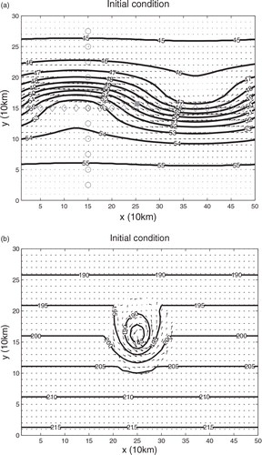
Figure 1b shows the true initial condition of Case II. The background mean height is 200 m, and the background uniform wind speed in the x direction is 10 ms⁻¹; and there is no mean flow in the y direction. A parabolic-shaped height perturbation with a maximum value of 20 m and a length scale of ~100 km is introduced in the centre of the domain. The wind and height truth fields are also geostrophically balanced initially.

The initial height fields of the nudging state and the ensemble state are based on shape-preserving perturbations to the truth state. For the nudging state, the true perturbation centre is moved westward one grid point and southward two grid points, and a random error of Gaussian distribution with mean zero and variance 2.0 is added onto the maximum value of the truth and is used to scale the parabolic-shaped height perturbation. The initial height fields of the ensemble members have random errors with Gaussian distribution with zero mean and a variance of 2.0 multiplied by the grid spacing, placed onto the perturbation centre of the initial nudging state. Random errors with Gaussian distribution mean zero and variance 2.0 are also superimposed on the maximum value used to define the amplitude of the initial nudging height perturbation field. The initial wind fields are also derived from the initial height fields using the geostrophic relationship in both the nudging and the ensemble state. Note that the rank of the initial ensemble depends on the initial perturbation; the perturbations used here were only chosen to initialise an appropriate ensemble spread.

Periodic lateral boundary conditions are used at the west–east boundaries in both cases. Case I has a free-slip rigid wall boundary condition at the southern and northern boundaries where the height and u components are defined from the values one point inside the boundary. For Case II, the tendencies of height and wind components are set to zero at the south–north boundaries.

3.3. The truth state and simulated observations

Truth states for each case are generated by first integrating a finer-scale model with grid spacing of 1 km, grid dimensions of 511×301 and a time step of 1 s. For this purpose, the model initial fields have no random or phase errors. The simulated observations are then produced by adding random errors with a Gaussian distribution with zero mean and assumed variances onto the 1-km truth fields. The simulated observations for Case I have variances , and . The variances of the simulated observations in Case II are given by , and . These variances are around 10% of their mean values.

Four types of observation networks are tested in this study. The first observation network (OBSN I) has only one observation site, which is shown by the grey solid square near the domain centre in Fig. 1a. Instead of having the observation located right in the domain centre, random displacements within one coarse grid cell are added to the domain centre to produce the observation site. The second observation network (OBSN II) consists of 19 observations spaced 25 km apart along the centre latitude of the domain (y=150 km), and shown by the grey diamonds in Fig. 1a. This OBSN II is chosen as the default or baseline observation network. The grey circles in Fig. 1a represent the third observation network (OBSN III), which has 11 observations spaced 25 km apart in the north–south direction off-centre and at x=150 km. The last observation network (OBSN IV) combines the OBSN II and OBSN III networks. The baseline configuration observations are available every 3 h.

3.4. Verification data and metrics

The verification data, based on the 1-km truth model simulation, is available at every grid point of the 10-km coarse domain. For a given grid point on the coarse domain, the verification value is the average of the surrounding 10×10 grid points on the 1-km fine-scale truth domain. The RMS errors of height and wind are computed separately every minute. Because the signal (amplitude) of the unforced wave or vortex is decreased gradually over time by diffusion, the actual model RMS error computed versus the truth field decreases with time. Thus, a normalised RMS error is used here, which is defined as the actual RMS error divided by the domain standard deviation of the truth field.

However, as discussed in Part I, the RMS error is not the only measure of success of a data assimilation technique, because it may not reflect discontinuities or noise generation in the analysis caused by the data assimilation method. Thus, a discontinuity parameter (DP) defined in Part I is also used here. The DP is the average absolute value of the RMS error difference in the analysis one time step (30 s) before the observation time and that at the observation time. Therefore, this measure is able to quantitatively assess the magnitude of error spikes/discontinuities induced following the data insertion.

3.5. Summary of experiments

As shown in Table 1, five basic experiments are conducted in this study: (1) Control (CTRL), assimilating no observations; (2) Nudging, using traditional observation nudging to relax the model state to the observations gradually with a fixed nudging strength 10⁻⁴ s⁻¹ and an isotropic Cressman-type influence function defined by a radius of influence (Stauffer and Seaman, 1994); (3) EnKF, assimilating the observations using the EnKF; (4) HNEnKF, assimilating the observations by the HNEnKF approach; and (5) EnKS, assimilating the observations by the lagged EnKS. Experiments CTRL and Nudging are single model experiments, while Experiments EnKF, HNEnKF and EnKS use an ensemble of model forecasts. Experiments are conducted first for a baseline configuration using 3-hourly observations and an observation network consisting of an east–west line of observations spaced 25 km apart at the central latitude (OBSN II). Observation frequencies of hourly and 6-hourly and three other observation networks (OBSN I, OBSN III and OBSN IV, see Section 3.3) are also applied as sensitivity tests to the above baseline experiments. The ensemble size is set to 20 for all experiments.

Table 1. Experimental design

Experimental name	Experimental description
CTRL	Assimilate no observations
Nudging	Assimilate observations by observation nudging with nudging coefficients of 10^−4 s^−1
EnKF	Assimilate observations by ensemble Kalman filter
HNEnKF	Assimilate observations by hybrid nudging-ensemble Kalman filter
EnKS	Assimilate observations by lagged ensemble Kalman smoother

The radius of influence for the observation nudging used in Experiment Nudging is specified to be the same as the error covariance localisation length scale of Experiment EnKF and HNEnKF defined further below. Both the Nudging and HNEnKF experiments have a 2-h nudging time window extending 1 h on each side of the observations. The trapezoidal temporal nudging coefficient function is defined by Stauffer and Seaman (1990) and applied as in Part I. It has a maximum weight of 1.0 within the centre half of the 2-h window, decreasing linearly to 0.0 at the ends of the window.

For the ensemble-based data assimilation experiments, to avoid filter divergence, the method suggested by Hamill et al. (2001) is used to increase the background error covariances somewhat by inflating the deviation of the background members with respect to their mean by a small amount (i.e. an inflation factor of 1.1 is used here). In addition, an error covariance localisation method is used following Houtekamer and Mitchell (2001), where a fifth-order piecewise rational function (Gaspari and Cohn, 1999) is used to scale the background error covariance. The error covariance localisation parameter 2c [see eq. (4.10) of Gaspari and Cohn (1999)] is set to 500 km, which is the wavelength in Case I. Similarly, Case II has the error covariance localisation parameter 2c set to 100 km, which is the scale of the initial vortex.

Following Khare et al. (2008), error covariance inflation is applied in the EnKS only to the prior estimates of the EnKF, and it is also set to 1.1. For efficiency, a lagged EnKS is applied here, which applies each observation backward only to the previous observation time every 30 minutes.

4. Results

We begin by applying a baseline 24-h model dynamic analysis assimilating 3-hourly observations from OBSN II (east–west line of observations at central latitude) to the wave case (Case I) and the moving vortex case (Case II) described in Section 3.2. The performance of the HNEnKF method is compared to that of the observation nudging and EnKF applied separately, and also to the EnKS.

In subsequent subsections, we further investigate the HNEnKF using a set of sensitivity tests by changing either the observation frequency or the observation network from the baseline configuration. The observation frequency (OBSF) varies from 3-hourly observations (OBSF 3) in the baseline to hourly observations (OBSF 1) and 6-hourly observations (OBSF 6). The four types of observation networks (OBSN) described in Section 3.3 are then tested.

4.1. Baseline results

Fig. 2 shows the normalised RMS errors of height and wind for the set of experiments in Table 1 for the wave Case I. Experiment Nudging fails to reduce the RMS error of either the height or wind fields (see discussion further below), while Experiment EnKF shows a significant error reduction every 3 h when observations are assimilated as evidenced by the strong RMS error decreases at the observation times. However, a rapid increase in error is evident soon after the observations are assimilated. This pattern is consistent with the 6-h assimilation period results in Fig. 1 of Fujita et al. (2007) using MM5 (Grell et al. 1994). It is also consistent with the presence of error spikes around the observation times shown in the Lorenz system results in Part I. By comparison, Experiment HNEnKF combining the EnKF and the continuous nudging approach shows the RMS error decreasing smoothly in time. The RMS errors of the HNEnKF experiment are lower than those of the EnKF experiment almost continuously after the first time the observations are assimilated. The dark grey dash-dotted vertical lines 30 minutes apart from Experiment EnKS denote the improvement in RMS error obtained by applying the next available observation back to the previous observation time. Since the next observation is applied backward only to the previous observation time every 30 minutes, the normalised RMS error of the EnKS is very similar to that of the EnKF, where large error corrections are made when observations are assimilated. Thus, the HNEnKF applied here produces smaller RMS errors throughout the assimilation period than either the EnKF or EnKS, and it also produces smoother analyses in time than both the EnKF and EnKS.

Fig. 2.  The normalised RMS error of Case I for Experiments CTRL (thin light grey solid line), Nudging (thick light grey solid line), EnKF (dark grey solid line), HNEnKF (black dash-dotted line) and EnKS (dark grey dash-dotted line). The baseline configuration (OBSF 3 and OBSN II) is used for all of the data assimilation experiments. (a) Height field and (b) wind field.

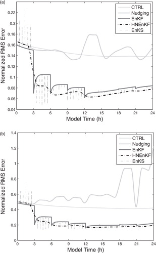
The normalised RMS errors of height and wind for the moving vortex Case II are shown in Fig. 3. It is interesting that the CTRL (using no data assimilation) performs best for the height field from the first observation time to the third observation time (Fig. 3a), followed by Experiments Nudging and HNEnKF. Note that the values for Experiments CTRL, Nudging and HNEnKF are from single-model experiments while EnKF and EnKS represent ensemble averages. Following the third observation time (9 h), Experiment HNEnKF shows a clear RMS error improvement in the height field over all the other data assimilation schemes. The wind field (Fig. 3b), however, responds more rapidly and decisively early in the simulation period to the data assimilation methods. These results suggest that the height field in Fig. 3a is likely to be adjusting more to the wind-field forcing than to the height observations directly. Unlike in Fig. 2b, Experiment Nudging is able to reduce the wind RMS error gradually in time compared to CTRL. As in the wave case of Fig. 2, strong adjustments by the EnKF at the observation times in Case II are seen in the wind field, and Experiment EnKS has strong error corrections when observations are assimilated. Similar to the wave case shown in Fig. 2b, the HNEnKF approach has smaller wind RMS error than the EnKF and EnKS, and it reduces the wind RMS error smoothly in time with fewer and weaker discontinuities compared to the EnKF and EnKS.

Fig. 3.  Same as Fig. 2, except for Case II.

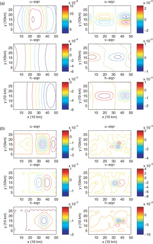
To explain why the observation nudging does not reduce the RMS error in Case I (Fig. 2), but does decrease the error in Case II (Fig. 3), the sums of nudging tendency terms in each equation of eq. (5) are shown on the whole domain for Experiments Nudging and HNEnKF at the first observation time (3 h) for both Case I and Case II (Fig. 4). Fig. 4a indicates that the sums of nudging tendency terms from Experiment Nudging are quite different from those of Experiment HNEnKF in Case I. For instance, the sums in the u equation for Nudging are positive on every grid point, but those of HNEnKF show dipole patterns with positive and negative values. As discussed before, HNEnKF reduces the RMS error successfully while Nudging does not. Thus, the specified nudging coefficients in Nudging do not appear to represent the error correlations realistically in Case I. In Fig. 4b, the sums of the nudging tendency terms in Nudging are more similar to those of the HNEnKF in Case II. For example, the sums of nudging tendency terms of Nudging in the v equation have a negative maximum around grid point (30, 15) and positive maximum around grid point (40, 14), which are located close to those of the HNEnKF. Fig. 3b shows both the Nudging and HNEnKF reducing the wind RMS error, although HNEnKF has lower wind RMS error than Nudging. Thus, the specified nudging coefficients in Case II for Experiment Nudging are better able to capture the more realistic error correlations computed by HNEnKF. This demonstrates that nudging, used alone with simple isotropic weighting, may have difficulty adapting to the non-isotropic error structure often encountered in a simulation.

Fig. 4.  The sums of nudging tendency terms from eq. (5) at every grid point at the first observation time (3 h) of the baseline simulation. (a) Case I and (b) Case II. The left column shows the sums of the nudging terms for each equation u, v and h from Experiment Nudging, and the right column shows the sums of the three hybrid nudging terms for each equation u, v and h from Experiment HNEnKF.

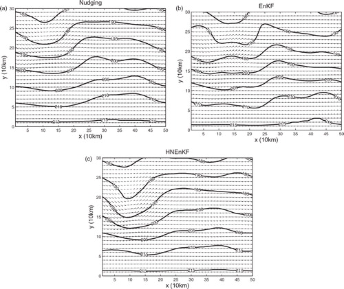
For the moving vortex Case II, the analyses of the Truth, CTRL and the data assimilation experiments at the end of simulation are shown in Fig. 5. The analysis of the EnKS is not shown, since it is the same as that of the EnKF at the end of simulation. Instead of having a trough at around x=70 km, the CTRL for Case II has a ridge there. The trough produced by the CTRL is further east than the Truth and strengthens towards the south. The HNEnKF produces the closest result to the Truth regarding the phase, orientation and strength of the trough, followed by the Nudging. The trough produced by the EnKF is further east and meanders from north to south rather than having a spatially coherent north–south orientation as in the Truth. These results are qualitatively consistent with those of the normalised RMS error comparison shown in Fig. 3.

Fig. 5.  The height and wind fields of Case II at the end of the dynamic analysis using the baseline configuration. (a) Truth, (b) CTRL, (c) Nudging, (d) EnKF and (e) HNEnKF.

In both the wave Case I and the vortex Case II, the baseline HNEnKF is able to produce smaller RMS errors throughout the 24-h period than the other data assimilation experiments (Nudging, EnKF and EnKS). It also produces a smoother analysis in time than either the EnKF or EnKS, because it has smaller discontinuities around the observation times than the EnKF and EnKS. Thus, the hybrid combination of nudging and the EnKF produces a dynamic analysis with lower errors than the nudging and EnKF applied separately.

4.2. Sensitivity to observation frequency

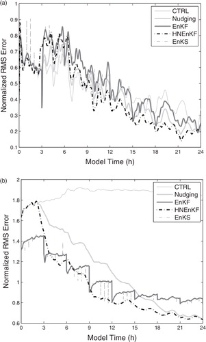
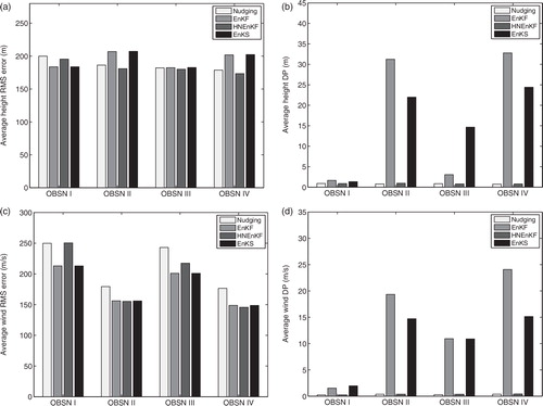
In this section, the data assimilation methods are explored with various observation frequencies or intervals using the baseline OBSN II in both Case I and Case II, since the performances of the data assimilation methods may vary with different observation frequencies, and real observations typically have different frequencies. The baseline observation frequency is every 3 h (OBSF 3), and observation frequencies of every 1 h (OBSF 1) and every 6 h (OBSF 6) are now tested. In Fig. 6, the average RMS error computed every minute and the DP computed at every observation time for the height and wind fields for wave Case I are shown. For each observation frequency, Experiments HNEnKF, EnKF and EnKS have lower average RMS errors than Experiment Nudging in both the height and wind fields, since the specified constant nudging coefficients poorly represent the error correlations as discussed in Section 4.1. Experiment HNEnKF has the lowest average height and wind RMS errors for all three observation frequencies. Experiments HNEnKF and Nudging have much smaller values of DP (fewer/smaller discontinuities) than Experiments EnKF and EnKS in both the height and wind fields for all three observation frequencies, especially when observation frequencies are every 3 h and every 6 h.

Fig. 6.  Height and wind RMS error and DP for Case I and Experiments Nudging, EnKF, HNEnKF and EnKS with different observation frequencies. (a) The average height RMS error, (b) the average height DP, (c) the average wind RMS error and (d) the average wind DP. Smaller values are better values for both average RMS error and DP.

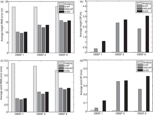
The RMS error and DP for vortex Case II are shown in Fig. 7. As discussed in Section 4.1, the specified nudging coefficients for this case appear to better represent the error correlations than those for Case I. Thus, the Nudging experiment has similar average height RMS errors to the HNEnKF (Fig. 7a), and similar or larger average wind RMS errors than the HNEnKF (Fig. 7c). Experiment HNEnKF produces lower average height RMS errors than the EnKF and EnKS for the three observation frequencies. The HNEnKF has similar average wind RMS errors to the EnKF and EnKS when observation frequencies are every 3 h and every 6 h, although it has larger average wind RMS errors than the EnKF and EnKS when the observation frequency is increased to 1 h. From Fig. 3b, the EnKF and EnKS were found to have an advantage in their average RMS errors through the first 3 h because of the ensemble averaging compared to the single model used by Nudging and HNEnKF, and this affects the average statistics over the entire model period shown in Fig. 7. As in Fig. 7b, d, the HNEnKF and Nudging show much smaller values of DP (fewer/smaller discontinuities) than the EnKF and EnKS in the height field (Fig. 7b) and wind field (Fig. 7d). These characteristics of the HNEnKF are attractive for the diagnostic dynamic studies and research studies using air-quality and atmospheric-transport and dispersion modelling.

Fig. 7.  Same as Fig. 6, except for Case II.

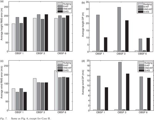
As mentioned in Section 3.5, the EnKS applies each observation backward to the previous observation time every 30 minutes. Then, to give the EnKS the greatest advantage, the average RMS errors of the height and wind fields can also be computed every 30 minutes. However, the 30-minute EnKS results are still similar to those presented above (not shown). Thus, generally the HNEnKF is able to produce lower average RMS error and improved (smaller) values of DP than the EnKF and EnKS in Case I and Case II regardless of the observation frequency.

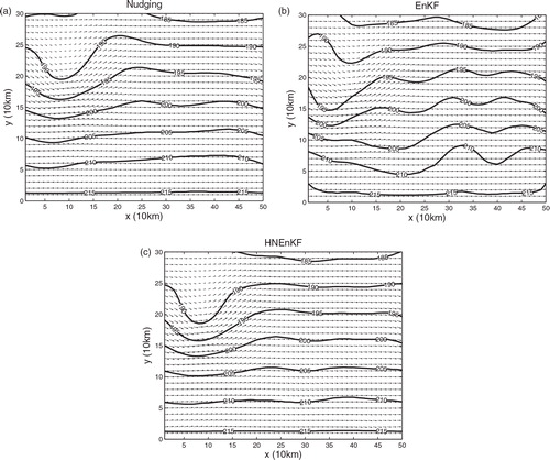
The analyses of the Nudging, EnKF and HNEnKF of Case II with OBSF 1 at the end of simulation are shown by Fig. 8. Both the HNEnKF and Nudging produce similar analyses to the Truth, while the trough produced by the HNEnKF is closer in the north–south gradient to the Truth than the Nudging. The height field from the ensemble mean of the EnKF exhibits more short wave energy than that of the Truth, HNEnKF and Nudging. The EnKF produces a weaker trough somewhat west than that of the Truth. Comparison with Fig. 5 reveals that all data assimilation experiments have improved analyses at the end of simulation due to more frequent observations being assimilated.

Fig. 8.  The height and wind fields of Case II at the end of the dynamic analysis for baseline configuration except using OBSF 1. (a) Nudging, (b) EnKF and (c) HNEnKF.

4.3. Sensitivity to observation network

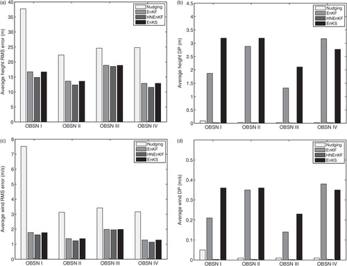
With the baseline 3-hourly observation frequency, the data assimilation methods are now applied with the various observation networks discussed in Section 3.3, in order to simulate the real observation networks that have sparse and dense data-density regions. Fig. 9 shows the average values of RMS error and DP over the 24-h period for Case I using the different observation networks for the data assimilation experiments. Fig. 9a, c shows that Experiment HNEnKF produces the smallest average RMS error in both the height and wind fields for all four observation networks. Fig. 9b, d indicates that the HNEnKF has the smallest values of DP, which means the best temporal smoothness of the dynamic analyses. The EnKF and EnKS have much larger values of DP than both the Nudging and HNEnKF. The EnKS usually has slightly smaller RMS errors than the EnKF at the analysis steps due to future observations being applied backward, and the lagged EnKS applies the next observation backward every 30 minutes instead of every time step. This explains why the EnKS has even larger values of DP than the EnKF. The HNEnKF retains the benefits of the EnKF by using flow-dependent and time-dependent error covariances that effectively reduce the RMS error, and it also yields a more seamless analysis by producing a smoother solution in time with smaller/fewer discontinuities than the EnKF by using nudging-type terms to apply the EnKF corrections continuously in time.

Fig. 9.  Height and wind RMS error and DP for Case I and Experiments Nudging, EnKF, HNEnKF and EnKS with different observation networks. (a) The average height RMS error, (b) the average height DP, (c) the average wind RMS error and (d) the average wind DP.

Figure 10 shows the average values of RMS error and DP for the moving vortex Case II when assimilating observations from the different observation networks. The HNEnKF produces the smallest average height and wind RMS errors in OBSN II and OBSN IV. However in OBSN I (for height and wind) and OBSN III (for wind), the HNEnKF produces larger average RMS errors than the EnKF and EnKS. This is likely because the error reduction in the EnKF and EnKS mainly comes from ensemble averaging, as shown in Fig. 3b in the first 3 h when no observations are assimilated. In addition, the observations in OBSN I and OBSN III play a much reduced role compared to the larger number of observations along the direction of the mean flow in OBSN II and OBSN IV. Obviously, the OBSN I and OBSN III networks cannot detect the eastward moving vortex sufficiently. Nonetheless, as shown in Fig. 10b,d, the HNEnKF still has lower, more desirable DP than the EnKF and EnKS, even with OBSN I and OBSN III.

Fig. 10.  Same as Fig. 9, except for Case II.

The analyses of the Nudging, EnKF and HNEnKF of Case II with OBSN IV at the end of simulation are shown in Fig. 11. Regarding the phase, orientation and strength of the trough, the HNEnKF produces the closest results to the Truth, followed by the Nudging. The EnKF is unable to produce a trough with coherent structure and orientation similar to that of the Truth. Comparison to Fig. 5 indicates that all data assimilation experiments have generally similar analyses to those with OBSN II, while the HNEnKF has better trough amplitude than that with OBSN II. This is because the OBSN III added to OBSN II to define OBSN IV cannot detect the eastward moving vortex sufficiently; thus, the north–south line of observations in OBSN III does not provide much useful information, and there is greater benefit from adding more observations in time to the OBSN II east–west distribution of observations (Fig. 8).

Fig. 11.  The height and wind fields of Case II at the end of the dynamic analysis for baseline configuration except using OBSN IV. (a) Nudging, (b) EnKF and (c) HNEnKF.

4.4. Relationship between ensemble spread and forecast error

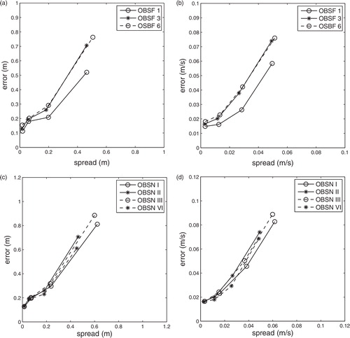
To ensure the EnKF and HNEnKF function properly, the ensemble forecast spread is compared to the forecast error of the ensemble mean. Instead of using scatterplots as in Part I, we plot the range of the ensemble spread and forecast error following Wang and Bishop (2003), because the larger number of points and overstamps for these 2-D model results make interpretation of scatterplots more difficult. We start from a scatterplot of points for which the abscissa of each point is given by the ensemble spread and the ordinate by the forecast error for each grid point at every analysis time. These points are then sorted in the order of increasing ensemble spread, and then divided into four equally populated bins. Then, the average values of the ensemble spread and forecast error in each bin are computed and plotted.

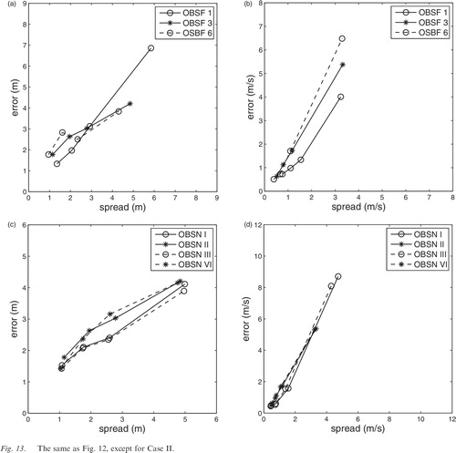
The relationships between the ensemble spread and forecast error of each group of sensitivity experiments of Case I and Case II are shown in Figs. 12 and 13, respectively. Given different observation frequencies (Fig. 12a,b) and observation networks (Fig. 12c, d), we find that the ensemble spread has an approximately linear correlation to the forecast error with a slope somewhat larger than 1 in Case I for both height and wind fields. In Case II, we again see the ensemble spread having an approximately linear correlation to the forecast error given different observation frequencies (Fig. 13a, b) and observation networks (Fig. 13c, d). The slopes of the height field are close to 1, while those of the wind field are somewhat larger than 1. Therefore, for the two groups of sensitivity experiments, the ensemble spread generally provides a reasonable estimate of the forecast error. We emphasise that these results are based on only two cases, and many more cases are needed to truly assess the spread–error relationship of an ensemble.

Fig. 12.  The range of ensemble spread and forecast error for the height and wind fields of the EnKF in Case I. (a) Height field with different observation frequencies, (b) wind field with different observation frequencies, (c) height field with different observation networks and (d) wind field with different observation networks.

5. Analysis of dynamic balance following data insertion

The motivation for developing the HNEnKF method is that an improved analysis with greater temporal smoothness and inter-variable consistency can be obtained if the data are applied gradually and continuously within a model using nudging-type terms that have been conditioned using the error covariance matrix of the EnKF. These terms can reduce dynamic imbalances and insertion shocks caused by intermittent data assimilation approaches. A calculation of the magnitude of the pressure tendencies or vertical motions in a mesoscale model is often performed to analyse the dynamic imbalances or noise introduced by the data insertion (e.g. Chen and Huang, 2006). Here in the shallow-water model, the evolution of the ageostrophic winds is used to quantify the effects of data insertion on the model balance.

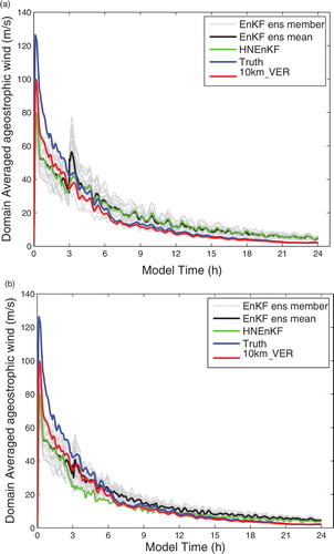
Fig. 13.  The same as Fig. 12, except for Case II.

To better investigate the impact of the data insertion on the dynamic balance that takes place through the model adjustment and induction processes due to few observation systems providing both mass and wind data, we evaluate the impact of assimilating only height observations or only wind observations at the third hour. The baseline model configuration using an east–west line of observations along the mean flow (OBSN II) is applied here to both cases. The magnitude of the ageostrophic winds is computed every time step at each grid point for the truth state at 1-km horizontal grid spacing and the data assimilation experiments at 10-km grid spacing. The verification data obtained by simply averaging the neighbouring 10×10 1-km grid points from the truth to the 10-km grid are also used to compute the ageostrophic winds (10km_VER). The ageostrophic wind is the difference between the geostrophic wind computed from the model (or verification data) height field and the model (or verification data) wind field. Then, the magnitude of the ageostrophic wind is averaged over the domain.

Figure 14a shows the evolution of domain-averaged ageostrophic wind speed in wave Case I when only height observations are assimilated at the third hour. It is clearly shown that the ensemble members using the EnKF (greylines) have dynamic imbalances/strong ageostrophic winds following the data assimilation. The ensemble mean (black line) also shows a discontinuity or noise burst after 3 h. By comparison, Experiment HNEnKF (green line) has the ageostrophic wind gradually evolving in time following the data insertion, which qualitatively follows the truth (blue line) and the 10km_VER but has a higher magnitude (red line). The time evolution of the ageostrophic wind following the data insertion represents the dynamic balance effects of the data assimilation. The larger magnitudes of the domain-averaged ageostrophic wind from the data assimilation experiments, compared to the 1-km truth, are mainly caused by coarser resolution effects, as seen by comparing the truth (blue) to the 10km_VER (red).

Fig. 14.  The domain-averaged ageostrophic wind computed for Case I for Experiments EnKF (each ensemble member in light grey, and the ensemble mean in black), HNEnKF (green), and the 1-km Truth (blue) and the 10-km_VER (red). (a) assimilating height observations only and (b) assimilating wind observations only.

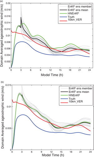
Figure 14b shows that when only wind observations are assimilated at the third hour in the wave Case I, a few ensemble members have a strong discontinuity in the agesotrophic wind, but the noise burst in the ensemble mean is not as obvious as when only height observations are assimilated. By comparison of Fig. 14b to Fig. 14a, the model adjustments appear to come more from the height field observations at this time for this case than the wind field observations. The HNEnKF still shows the ageostrophic wind varying smoothly in time, similar to when only height observations were assimilated.

The domain-averaged ageostrophic wind in the vortex Case II is shown in Fig. 15. When only height observations are assimilated (Fig. 15a), the ensemble members of EnKF and their ensemble mean again have a strong discontinuity in the ageostrophic wind. By comparison, the HNEnKF shows a much smaller effect: the ageostrophic wind decreases gradually following the data insertion, very similar to that of the truth and 10km_VER. Similar to Case I, the difference in the ageostrophic wind magnitude between the data assimilation experiments and the truth mainly comes from the grid resolution. When only wind observations are assimilated (Fig. 15b), there are also ageostrophic wind bursts in the ensemble members and their ensemble mean, although the magnitudes of the discontinuities are not as large as those obtained when assimilating height observations only. The HNEnKF again performs similarly to the truth and 10km_VER that have the ageostrophic wind evolving gradually in time without any large discontinuities.

Fig. 15.  Same as Fig. 14, except for Case II.

Thus, the EnKF, an intermittent data assimilation method, experiences larger dynamic imbalances and ageostrophic wind tendencies in the model state following the observation time compared to the continuous HNEnKF method. The HNEnKF is able to better maintain the dynamic balance by gradually applying nudging-type terms that have been computed using the error covariance matrix of the EnKF, thus producing a more continuous and seamless analysis in time.

6. Computational efficiency

As discussed in Part I, the EnKF, HNEnKF and EnKS experiments utilise an ensemble forecast that is more computationally expensive than a single model run as used in Experiment Nudging. The EnKS is even more CPU-intensive than the EnKF and HNEnKF and also requires greater storage proportional to the total number of analysis times over which the statistics are used. Similar to Part I, the computational efficiency of these data assimilation methods is discussed in this section.

Table 2 shows the CPU time cost of the various data assimilation schemes using the baseline configuration. The Nudging has the smallest CPU time cost, because it does not require an ensemble of forecasts. The HNEnKF has similar CPU time cost to the EnKF, since both involve an ensemble forecast. These results are consistent with those of Part I. The EnKS has a CPU time cost around 2.5 times that of the EnKF and HNEnKF. We would expect smaller RMS error and DP of the EnKS if it is operated as in Part I by applying future observations backward to the initial time every time step. The relative CPU time cost of EnKS is much smaller here than that of Part I, because the more practical, lagged EnKS used here only applies each observation backward to the previous observation time every 30 minutes. The HNEnKF produces similar or better RMS error and DP than the lagged EnKS, but with reduced CPU time and storage costs.

Table 2. Total CPU time cost of different data assimilation schemes with baseline configuration

Experiment	Nudging	EnKF	HNEnKF	EnKS
CPU time (s)	47	298	299	732

7. Conclusions

The HNEnKF data assimilation approach, introduced in Part I for the three-variable Lorenz system, is further investigated here using a 2-D shallow-water model with a 20-member ensemble. The HNEnKF combines the advantages of both the EnKF and nudging by applying the EnKF gradually in time via nudging-type terms. The HNEnKF uses the EnKF to provide flow-dependent and time-dependent nudging coefficients and also includes non-zero off-diagonal elements for better inter-variable influences from the innovations.

A quasi-stationary wave case (Case I) and a moving vortex case (Case II) are used to test the HNEnKF method for dynamic analysis and NWP-type applications. The HNEnKF in the baseline configuration (3-hourly observations and OBSN II) generally reduces the RMS errors through the 24-h period more than the nudging and EnKF applied separately. Moreover, the HNEnKF retains the benefits from the EnKF while using a continuous assimilation to improve the model state gradually rather than making strong corrections and discontinuities at the analysis steps as with the intermittent EnKF assimilation. Thus, it has smaller (better) values of the DP than the EnKF. The HNEnKF also produces lower DP (better temporal smoothness) than the reduced-cost lagged EnKS. Moreover, the average RMS errors in the 24-h HNEnKF simulations are comparable or lower than those of the EnKS used in this study. The HNEnKF is comparable in cost to the EnKF, and both the HNEnKF and EnKF yield smaller CPU time and storage costs than the EnKS.

Sensitivity experiments using different observation frequencies (OBSF 1, OBSF 3 and OBSF 6) and observation networks (OBSN I, OBSN II, OBSN III and OBSN IV) are also performed. In general, the results found in the baseline HNEnKF simulations for producing comparable or smaller average RMS errors throughout the 24-h period and smaller (better) values of DP than the EnKF and EnKS around the analysis times are confirmed.

To ensure that the EnKF and HNEnKF function properly, the ensemble spread is compared to the forecast error for each group of sensitivity experiments. The relationship between the ensemble spread and forecast error of the ensemble mean is approximately linear with slopes close to or somewhat larger than 1. Thus, the ensemble spread provides a reasonable estimate of the forecast error. Again we emphasise that many more cases are needed to truly assess the spread–error relationship for an ensemble and its effect on the ensemble-based data assimilation methods, and calibration of the spread–error relationship may also be needed (e.g. Kolczynski et al., 2009, 2011).

The added value of the HNEnKF over the EnKF is further investigated by analysing the effects of the data assimilation methods on the model dynamic balance (i.e. evolution of the ageostrophic winds) following the assimilation of only wind data or only mass data. The EnKF, as an intermittent data assimilation approach, has strong discontinuities in the model state at the analysis times, as shown by the bursts in the domain-averaged ageostrophic winds. By comparison, the HNEnKF, which applies the error covariance information of the EnKF gradually in time, produces a smooth evolution of the ageostrophic wind, without any strong discontinuities following the data insertion, more like the ageostrophic wind in the truth and 10-km verification data. Thus, it is demonstrated that the continuous HNEnKF produces seamless analyses with a greater degree of dynamic balance compared to the EnKF. Building on these encouraging results in Parts I and II, we are now applying this HNEnKF approach to real data in the 3-D WRF model, and these results will be reported in another paper (accepted by Quart. J. Roy. Meteor. Soc.).

The advantages of this continuous HNEnKF come from the hybrid nudging technique applied to the single-member nudging state. However, the ensemble state has a similar insertion noise problem to the EnKF, because it is updated by the intermittent EnKF. This imbalance in the ensemble state may limit its ability to provide good hybrid nudging coefficients to the nudging state. Thus, future work should investigate decreasing the insertion noise in members of the ensemble state on the performance of the HNEnKF.

Future work will also explore the application of this HNEnKF approach for improving forecasts, since the HNEnKF was mainly investigated in dynamic-analysis mode in Parts I and II. In a dynamic-forecast mode, the HNEnKF could be used to better initialise and spin up the subsequent forecasts. Both the nudging state and ensemble state will be used together to assimilate real-time observations during a pre-forecast period. The HNEnKF will integrate the nudging state to the current forecast initialisation time using the observations within this period and the hybrid nudging coefficients from the EnKF. The HNEnKF will then update the ensemble state from the EnKF simultaneously. This forecast-analysis cycle can be repeated in a real-time operational environment as the observations become available within the pre-forecast period.

Acknowledgements

This research was supported by DTRA contract No. HDTRA1-07-C-0076 under the supervision of John Hannan of DTRA. The authors would like to thank George Young, Sue Ellen Haupt, Nelson Seaman and Fuqing Zhang for helpful discussions and comments.

References

- Anderson J. L. An ensemble adjustment Kalman filter for data assimilation. Mon. Wea. Rev. 2001; 129: 2884–2903. 10.3402/tellusa.v64i0.18485.
- Arakawa A. Lamb V. Computational design of the basic dynamical processes in the UCAL general circulation model. Methods Comput. Phys. 1977; 17: 174–264.
- Auroux D. Blum J. A nudging-based data assimilation method: the back and forth (BFN) algorithm. Nonlin. Processes Geophys. 2008; 15: 305–319. 10.3402/tellusa.v64i0.18485.
- Ballabrera-Poy J. Kalnay E. Yang S. Data assimilation in a system with two scales – combining two initialization techniques. Tellus. 2009; 61A: 539–549.
- Chen M. Huang X. Digital filter initialization for MM5. Mon. Wea. Rev. 2006; 134: 1222–1236. 10.3402/tellusa.v64i0.18485.
- Chin T. M. Turmon M. J. Jewell J. B. Ghil M. An ensemble-based smoother with retrospectively updated weights for highly nonlinear system. Mon. Wea. Rev. 2007; 135: 186–202. 10.3402/tellusa.v64i0.18485.
- Colle B. A. Mass C. F. The 5–9 February 1996 flooding event over the Pacific Northwest: sensitivity studies and evaluation of the MM5 precipitation forecasts. Mon. Wea. Rev. 2000a; 128: 593–617. 10.3402/tellusa.v64i0.18485.
- Colle B. A. Mass C. F. High-resolution observations and numerical simulations of easterly gap flow through the Strait of Juan de Fuca on 9-10 December 1995. Mon. Wea. Rev. 2000b; 128: 2363–2396. 10.3402/tellusa.v64i0.18485.
- Deng A. Seaman N. L. Hunter G. K. Stauffer D. R. Evaluation of interregional transport using the MM5-SCIPUFF system. J. Appl. Meteor. 2004; 43: 1864–1886. 10.3402/tellusa.v64i0.18485.
- Dixon M. Li Z. Lean H. Roberts N. Ballard S. Impact of data assimilation on forecasting convection over the United Kingdom using a high-resolution version of the Met office unified model. Mon. Wea. Rev. 2009; 137: 1562–1584. 10.3402/tellusa.v64i0.18485.
- Duane G. S. Tribbia J. J. Weiss J. B. Synchronicity in predictive modeling: a new view of data assimilation. Nonlin. Processes Geophys. 2006; 13: 601–612. 10.3402/tellusa.v64i0.18485.
- Evensen G. Sequential data assimilation with a nonlinear quasi-geostrophic model using Monte Carlo methods to forecast error statistics. J. Geophys. Res. 1994; 99C5: 10143–10162. 10.3402/tellusa.v64i0.18485.
- Evensen G. van Leeuwen P. J. An ensemble Kalman smoother for nonlinear dynamics. Mon. Wea. Rev. 2000; 128: 1852–1867. 10.3402/tellusa.v64i0.18485.
- Fujita T. Stensrud D. J. Dowell D. C. Surface data assimilation using an ensemble Kalman filter approach with initial condition and model physics uncertainties. Mon. Wea. Rev. 2007; 135: 1846–1868. 10.3402/tellusa.v64i0.18485.
- Gaspari G. Cohn S. E. Construction of correlation functions in two and three dimensions. Quart. J. Roy. Meteor. Soc. 1999; 125: 723–757. 10.3402/tellusa.v64i0.18485.
- Grammeltvedt A. A survey of finite-difference schemes for the primitive equations for a barotropic fluid. Mon. Wea. Rev. 1969; 97: 384–404. 10.3402/tellusa.v64i0.18485.
- Grell, G. A, Dudhia, J and Stauffer, D. R. 1994. A description of the fifth-generation Penn State/NCAR Mesoscale Model (MM5). NCAR Tech. Note NCAR/TN-398, 128. pp.
- Hamill T. M. Whitaker J. S. Snyder C. Distance-dependent filtering of background error covariance estimate in an ensemble Kalman filter. Mon. Wea. Rev. 2001; 1298: 2776–2790. 10.3402/tellusa.v64i0.18485.
- Houtekamer P. L. Mitchell H. L. Data assimilation using an ensemble Kalman filter technique. Mon. Wea. Rev. 1998; 126: 796–811. 10.3402/tellusa.v64i0.18485.
- Houtekamer P. L. Mitchell H. L. A sequential ensemble Kalman filter for atmospheric data assimilation. Mon. Wea. Rev. 2001; 129: 123–137. 10.3402/tellusa.v64i0.18485.
- Hunt, B. R, Kalnay, E, Kostelich, E. J, Ott, E, Patil, D. J and co-authors. 2004. Four-dimensional ensemble Kalman filtering. Tellus. 56A, 273–277.
- Juckes M. Lawrence B. Inferred variables in data assimilation: quantifying sensitivity to inaccurate error statistics. Tellus. 2009; 61A: 129–143.
- Khare S. P. Anderson J. L. Hoar T. J. Nychka D. An investigation into the application of an ensemble Kalman smoother to high-dimensional geophysical systems. Tellus. 2008; 60A: 97–112.
- Kolczynski, W. C. Jr, Stauffer, D. R, Haupt, S. E, Altman, N. S and Deng, A. 2011. Investigation of ensemble variance as a measure of true forecast variance. Accepted for publication in. Mon. Wea. Rev. 139, 3954–3963. 10.3402/tellusa.v64i0.18485.
- Kolczynski W. C. Jr. Stauffer D. R. Haupt S. E. Deng A. Ensemble variance calibration for representing meteorological uncertainty for Atmospheric Transport and Dispersion modeling. J. Appl. Meteor. 2009; 48: 2001–2021. 10.3402/tellusa.v64i0.18485.
- Lei, L, Stauffer, D. R, Haupt, S. E and Young, G. S. 2012. A hybrid nudging-ensemble Kalman filter approach to data assimilation. Part I: application in the Lorenz system. Tellus A 2012, 64, 18484, http://dx.doi.org/10.3402/tellusa.v64i0.18484.
- Monaghan A. Rife D. L. Pinto J. O. Davis C. A. Hannon J. R. Global precipitation extremes associated with diurnally varying low-level jets. J. Climate. 2010; 23: 5065–5084. 10.3402/tellusa.v64i0.18485.
- Otte T. L. The Impact of nudging in the meteorological model for retrospective air quality simulations. Part I: evaluation against national observation networks. J. Appl. Meteor. Climatol. 2008a; 47: 1853–1867. 10.3402/tellusa.v64i0.18485.
- Otte T. L. The Impact of nudging in the meteorological model for retrospective air quality simulations. Part II: evaluating collocated meteorological and air quality observations. J. Appl. Meteor. Climatol. 2008b; 47: 1868–1887. 10.3402/tellusa.v64i0.18485.
- Pleim J. E. Gilliam R. An indirect data assimilation scheme for deep soil temperature in the Pleim–Xiu land surface model. J. Appl. Meteor. Climatol. 2009; 48: 1362–1376. 10.3402/tellusa.v64i0.18485.
- Pu Z. Hacker J. Ensemble-based Kalman filters in strongly nonlinear dynamics. Adv. Atmos. Sci. 2009; 26: 373–380. 10.3402/tellusa.v64i0.18485.
- Rife D. L. Pinto J. O. Monaghan A. J. Davis C. A. Hannon J. R. Global distribution and characteristics of diurnally varying low-level jets. J. Climate. 2010; 23: 5041–5064. 10.3402/tellusa.v64i0.18485.
- Schroeder, A. J, Stauffer, D. R, Seaman, N. L, Deng, A, Gibbs, A. M and co-authors. 2006. An automated high-resolution, rapidly relocatable meteorological nowcasting and prediction system. Mon. Wea. Rev. 134, 1237–1265. 10.3402/tellusa.v64i0.18485.
- Skamarock, W. C, Klemp, J. B, Dudhia, J, Gill, D. O, Barker, D. M and co-authors. 2008. A Description of the Advanced Research WRF Version 3. NCAR Tech. Note. 125 pp. On line at: http://www.mmm.ucar.edu/wrf/users/docs/arw_v3.pdf.
- Stauffer D. R. Bao J.-W. Optimal determination of nudging coefficients using the adjoint equations. Tellus. 1993; 45A: 358–369.
- Stauffer D. R. Seaman N. L. Use of four-dimensional data assimilation in a limited-area mesoscale model. Part I: experiments with synoptic data. Mon. Wea. Rev. 1990; 118: 1250–1277. 10.3402/tellusa.v64i0.18485.
- Stauffer D. R. Seaman N. L. Multiscale four-dimensional data assimilation. J. Appl. Meteor. 1994; 33: 416–434. 10.3402/tellusa.v64i0.18485.
- Stauffer D. R. Seaman N. L. Hunter G. K. Leidner S. M. Lario-Gibbs A. Tanrikulu S. A field-coherence technique for meteorological field-program design for air quality studies. Part I: description and interpretation. J. Appl. Meteor. 2000; 39: 297–316. 10.3402/tellusa.v64i0.18485.
- Tanrikulu S. Stauffer D. R. Seaman N. L. Ranzieri A. J. A field-coherence technique for meteorological field-program design for air-quality studies. Part II: evaluation in the San Joaquin Valley. J. Appl. Meteor. 2000; 39: 317–334. 10.3402/tellusa.v64i0.18485.
- Wang X. Bishop C. H. A comparison of breeding and ensemble transform Kalman filter ensemble forecast schemes. J. Atmos. Sci. 2003; 60: 1140–1158. 10.3402/tellusa.v64i0.18485.
- Whitaker J. S. Hamill T. M. Ensemble data assimilation without perturbed observations. Mon. Wea. Rev. 2002; 130: 1913–1924. 10.3402/tellusa.v64i0.18485.
- Yang, S, Baker, D, Li, H, Cordes, K, Huff, M and co-authors. 2006. Data assimilation as synchronization of truth and model: experiments with the three variable Lorenz system. J. Atmos. Sci. 63, 2340–2354. 10.3402/tellusa.v64i0.18485.
- Zhu K. Navon I. M. Zou X. Variational data assimilation with a variable resolution finite-element shallow-water equations mode. Mon. Wea. Rev. 1994; 122: 946–965. 10.3402/tellusa.v64i0.18485.
- Zou, X, Navon, I. M and Ledimet, F. X. 1992. An optimal nudging data assimilation scheme using parameter estimation. Quart. J. Roy. Met. Soc. 1992, 118, 1163–1186. 10.3402/tellusa.v64i0.18485.