North Atlantic variability driven by stochastic forcing in a simple model

ABSTRACT

This study investigates the mechanisms driving North Atlantic (NA) variability using a simple model that incorporates the time evolution of interactive upper ocean temperature anomalies, horizontal (Gyre, Ψ _g ) and vertical (meridional overturning circulation, Ψ _m ) circulation. The model is forced with multicentury long synthetic time series of external stochastic forcing that captures key statistical properties of observations such as the range of fluctuations and persistence of processes. The simulated oceanic response may be viewed as a delayed response to a cumulative atmospheric forcing over an interval defined by the system damping properties. Depending on the choice of parameters, the model suggests either compensatory mechanism (Ψ _m and Ψ _g are anti-correlated) or amplification mechanism (Ψ _m and Ψ _g are positively correlated). The compensatory mechanism implies that an increase of heat supplied by an anomalously strong Ψ _g would be balanced by a decrease of heat provided by a weaker Ψ _m and vice versa. The amplification mechanism suggests that both Ψ _m and Ψ _g maintain the heat budget in the system compensating its damping properties. Some evidence for these mechanisms is found in a global climate model. Further investigations of NA variability mechanisms are important as they improve understanding of how the NA climate system functions.

• North Atlantic
• stochastic modelling
• variability

1. Introduction

The North Atlantic Oscillation (NAO) is the leading mode of atmospheric variability over the North Atlantic (NA) and is defined as the normalised difference of sea level pressure between two centres of atmospheric action located around the Azores and Iceland (Rogers, 1984; Hurrell et al., 2002). The spatial pattern of the NAO is responsible for the atmospheric redistribution of surplus heat from the subtropical Atlantic to the Arctic. Positive and negative phases of the NAO are characterised by distinct spatial patterns of NA surface air temperature (SAT) and sea level pressure. A NAO+ (NAO −) phase is associated with a stronger (weaker) north–south pressure gradient between the subtropical high and the Icelandic low, resulting in an increase (decrease) of poleward heat transport by stronger (weaker) than average westerlies and oceanic circulation. Thus, the NAO+(NAO −) phase is associated with generally warmer (cooler) SATs and sea surface temperatures (SSTs) north of 45°N (Visbeck et al., 2002).

Numerous studies (e.g. Bjerknes, 1964; Deser and Blackmon, 1993; Kushnir, 1994; Dickson et al., 1996, 2002; Timmermann et al., 1998; Curry et al., 1998, 2003; Häkkinen, 1999; Curry and McCartney, 2001; Visbeck et al., 2002) point to the important role of the NAO in the North Atlantic Ocean variability. For example, Joyce et al. (2000) used observational data and found a decadal-scale covariability of the NAO and the SST signal produced by a shift of the Gulf Stream along its path. However, there are several competing hypotheses about potential mechanisms driving NA variability. Hasselmann (1976) proposed a stochastic model of climate variability, where atmospheric ‘weather’ forcing with essentially a white noise spectrum is integrated by the ocean and results in a redder climate response spectrum. This theory is supported by numerous later studies (e.g. Battisti et al., 1995; Griffies and Tziperman, 1995; Frankignoul and Hasselmann, 1977; Hall and Manabe, 1997; Jin, 1997; Barsugli and Battisti, 1998; Frankignoul et al., 1998; Saravan and McWilliams, 1998; Weng and Neelin, 1998; Cessi, 2000; Delworth and Greatbatch, 2000; Marshall et al., 2001). For example, the sensitivity study by Delworth and Greatbach (2000) demonstrated that multidecadal fluctuations of the NA thermohaline circulation may be viewed as a passive oceanic response to atmospheric surface flux forcing, whose pattern is associated with the NAO. Using different general circulation models (GCM), Dong and Sutton (2005) and Jungclaus et al. (2005) reached the same conclusion about the low-frequency variations of the NA meridional overturning circulation (MOC), which defines the largest portion of northward upper oceanic heat transport compensated by deep southward flow of coldwater.

However, there is mounting evidence that NA variability reflects a two-way interaction between the ocean and the atmosphere suggesting an active role of the ocean. For example, Barsugli and Battisti (1998) offered a simple model of mid-latitude air–sea interactions in which coupling between atmosphere and ocean reduces internal damping in the system resulting in greater thermal variance in the coupled atmosphere and ocean. Czaja and Frankignoul (1999) found evidence that a significant fraction (~25%) of winter NAO variance could be predicted from the prior basin-scale SST pattern. A sensitivity analysis by Frankignoul and Kestenare (2005) confirmed the robustness of influence of a horseshoe SST anomaly on the NAO pattern. Eden and Greatbatch (2003) using a realistic ocean model coupled with a simplified stochastic atmospheric model found a damped decadal oscillation in which oceanic processes played an active role.

At longer time scales, changes of oceanic thermohaline circulation play an important role in establishing spatial and temporal SST patterns (e.g. Delworth et al., 1993; Timmermann et al., 1998; Häkkinen, 1999; Eden and Jung, 2001; Eden and Greatbatch, 2003; Barnett et al., 2005; Knight et al., 2005; Hawkins and Sutton, 2007; Zhang et al., 2007). For example, Timmerman et al. (1998) using a general circulation model demonstrated a coupled atmosphere–ocean mode with a ~35-year cycle. In this mode, a weaker MOC leads to large-scale negative SST anomalies and a weakened NAO, which in turn causes positive surface salinity anomalies over convection sites and intensified MOC. Hence, the system is ready for the next half of the cycle. Eden and Greatbatch (2003) found a decadal signal in their NA coupled ocean–atmosphere model. The decadal oscillation was orchestrated by a fast wind-driven positive feedback of the ocean and delayed negative feedback due to overturning circulation anomalies. Danabasoglu (2008) and Zhu and Jungclaus (2008) also found low-frequency modes with active ocean–atmosphere interactions in two different climate models. However, recently Msadek and Frankignoul (2009) demonstrated (using yet another climate model) that even though the coupled air–sea mode is important in controlling the decadal to multidecadal variability in the NA, the NAO plays a secondary role in the MOC fluctuations. Polyakova et al. (2006) pointed to a lack of steadiness in the decadal-scale relationship between the NAO, SAT and SST over the NA region. Thus, there is no consensus on the role of the NAO in shaping the atmosphere–ocean interactions and low-frequency variability of the NA.

In this study, we investigate the NA variability driven by ocean–NAO interactions following a theoretical framework proposed by Marshall et al. (2001). The conceptual model of Marshall et al. explores fluctuations of NA SSTs in response to local air–sea interactions, anomalous advection of heat by horizontal (gyre) and vertical (MOC) cells of oceanic circulation, and overlying wind pattern including feedback mechanisms of anomalous SSTs on oceanic circulation.

Marshall et al. (2001) showed that a circulation anomaly called the ‘intergyre’ gyre is driven by meridional shifts in the zero wind stress curl, which is climatologically located between the subpolar and subtropical gyres. According to Marshall et al. (2001), the oscillatory behaviour of the intergyre gyre is governed by north–south heat transports by anomalous currents, balanced by damping of the SST anomalies via air–sea interactions. Marshall et al. (2001) hypothesised that the meridional shift of Gulf Stream may be responsible for intensification or weakening of the intergyre gyre. Polyakov et al. (2010) demonstrated that multidecadal variability of the zonal average temperatures and wind stress curl anomalies computed over the intergyre gyre region are negatively correlated (R = −0.44) at an 8-year lag. The authors argued that this is consistent with a delayed oceanic response to the atmospheric forcing found in modelling (Eden and Willebrand, 2001) and theoretical (Marshall et al., 2001) studies. Polyakov et al. (2010) showed that during prolonged phases of high (low) wind vorticity there is anomalous upwelling (downwelling) centred at ~45°N concurrent with lower (higher) SSTs and decreased (increased) surface heat fluxes out of the ocean. This pattern is consistent with the ocean response to the NAO simulated by general circulation models (e.g. Eden and Willebrand, 2001; Vellinga and Wu, 2004).

In this study, we explored the excitation of oceanic anomalies by a synthetic stochastic forcing that captures key statistical properties of actual observations. For each stochastic time series, a range of fluctuations was defined by observation-based standard deviations (SDs) whereas persistence of processes was incorporated into stochastic forcing via the Hurst exponent. Section 2 highlights important mechanisms of the conceptual model including the horizontal ocean gyre, vertical MOC and air–sea interaction mechanisms presented by Marshall et al. (2001). A description of the model experiments as well as the methods utilised in the development of stochastic forcings is included in Section 3. In the course of our study we explore the effects associated with each forcing and each term of the model separately. In this article (Section 4), we present key experimental results to highlight compensatory and amplification mechanisms between the horizontal gyre and vertical MOC circulation which both work hand-in-hand in order to maintain the heat balance within the system. This result may be viewed as complementary to the seminal study of air–sea interactions by Bjerknes (1964), and the subsequent theoretical exposition of the major themes developed by Bjerknes in the conceptual model by Marshall et al. (2001). Section 5 explores the question of whether the mechanisms from the simple stochastically forced model operate in the present day global climate models. In Section 6, we summarise the key results of our study.

2. Model description

In this study, we utilised a model proposed by Marshall et al. (2001). The model simulates changes in the intensity of North Atlantic Ocean circulation and upper ocean temperature anomalies in response to air–sea interactions. These interactions include the damping of upper ocean temperatures by latent and sensible heat fluxes at the air–sea interface, as well as Ekman heat transport in the upper ocean layers. Together these equations form the foundation of a simple box model used to describe the interactions and feedbacks between the model forcing and responding components.

Following Marshall et al. (2001), the upper North Atlantic Ocean is approximated by a box with an east–west dimension, L _x , of 3000 km, a north–south dimension, L _y , of 3000 km and a depth, h, of 200 m extending over the NA between 30–60°N and 80–0°W. The model divides the NA basin into north and south triangular ocean and atmosphere boxes following a Z-like pattern (Fig. 1). The triangles were split along a line that approximately coincides with the mean climatological zero wind stress line. Marshall et al. (2001) argued that the climatological anomalies in water temperature would be approximately equal and of opposite sign for the northern and southern boxes, and for simplification, the equations describing the model were set up for the northern triangle.

Fig. 1.  Schematic showing a Z-like pattern whose diagonal is the zero wind stress curl line based on wind climatology, and the top and bottom lines are the zero wind stress curl lines of the NAO anomaly. Regions of warming and cooling as well as the intergyre gyre spun up by the NAO+ are also indicated (from Marshall et al., 2001).

The model's eq. (1) describes the evolution in time t of the upper ocean heat content anomaly in the northern triangle of the domain (i.e. above the diagonal of the Z). These anomalies result from changes in the MOC, intensity of the horizontal ocean gyre (intergyre gyre) and external forcing of the atmosphere:1

where C _o =ρ _o c _o h is the heat capacity of the upper ocean, ρ _o is the density of water, c _o is its specific heat, A = (L _x L _y )/2 is the area of the northern triangle, T _oN is the water temperature anomaly, T _aN is synonymous to SAT and Ψ _g∣w is the (non-dimensional) westernmost value of the gyre streamfunction anomaly evaluated inside the western boundary current (Marshall et al., 2001). In this equation, Q _M , Q _G and Q _E are scales for heat transport due to anomalous thermohaline, gyral and Ekman circulation across the diagonal of the Z:2 3 4

where is the difference in the mean temperature over the MOC vertical extent, is the change in the mean SST along the climatological position of the mean zero curl line and is the difference in sea-surface temperature averaged across the basin at latitudes corresponding to the horizontal lines of the Z. is the non-dimensional measure of the strength of the MOC with respect to the scale Ψ _M =15 Sv (1 Sv =10⁶ m³ s⁻¹). are analogous quantities for the gyre circulation, Ψ _G =10 Sv. Ψ _G is evaluated by Marshall et al. (2001) via their eq. (A22) using other, better defined, scales like wind stress scale and horizontal basin dimensions. We note that the gyre circulation scale may be overestimated due to other factors (like baroclinicity, for example), which are not included in the relationship eq. (A22). f _o is the Coriolis parameter and is a non-dimensional measure of the surface wind stress with respect to the scale τ _wind =0.05 N m⁻² (Marshall et al., 2001). The air–sea flux (the fourth term in right-hand side of eq. 1) is expressed in the study of Marshall et al., (2001) in terms of the air–sea temperature difference with the linearised coefficient of combined latent and sensible heat flux λ _o,a used as a multiplier.

The ocean gyre (intergyre) streamfunction anomalies, Ψ _ig (i.e. anomalies of the horizontal cell of the circulation), are defined in eq. (5) incorporating both the time and space, x, evolution of Ψ _ig balanced by the surface wind stress transmitted to the ocean by Ekman pumping:5

where c _R =β L _ρ is the zonal phase speed of long, non-dispersive Rossby waves, L _ρ is the deformation radius, β is the meridional gradient of the Coriolis parameter f _o and Ekman pumping velocity, w _e , is given by:6

Equation (5) is similar to the eq. (3) from Frankignoul et al. (1997). The model neglects the barotropic response of the ocean gyre to external forcing. Using this model, Frankignoul et al. (1997) predicted power spectra of the NA baroclinic pressure variability whose shape and geographical features were broadly consistent with the spectra derived from global climate model simulations and observations. Marshall et al. (2001) provided arguments for the dominant role of the baroclinic velocities in advecting the temperature anomalies in the gyre's heat transports. We discuss the possible caveats and limitations of this approach in Section 4 in greater detail.

The MOC streamfunction anomalies, Φ (i.e. anomalies in the vertical cell of the circulation), are given by:7

where L _z is the vertical scale (=1000 m) of the Φ, α is the thermal expansion coefficient of water and is the effective acceleration of gravity acting on horizontal temperature gradients; Y = 1°C is the temperature anomaly scale, t _delay =L _x /c _R is the time scale defined as time required for Rossby waves to cross the domain and δT _o is temperature differences between the northern and southern boxes (Marshall et al., 2001).

Following Marshall et al. (2001), the basic equations of the model (i.e. eqs. 1, 5 and 7) are rewritten in dimensionless form. The scaling factors used to transfer dimensional variables to non-dimensional are presented in Table A1.8 9 10 11

where T is non-dimensional water temperature anomaly with respect to temperature anomaly scale, Y = 1°C, Ψ_moc =L _x Φ and S incorporated in s is (Marshall et al., 2001). The non-dimensional factors g and m describe the efficiency of heat transport by the horizontal gyre and MOC, while λ describes the effectiveness of damping of ocean temperature anomalies by air–sea interactions and feedback of Ekman layers. The factor s refers to the efficiency of the thermal ocean dipoles driving the meridional overturning in the basin. The factor f describes the feedback of ocean temperatures on wind stress. Other non-dimensional terms used in the model (including definitions for the above factors) along with the model variables used to define the model parameters are defined in Table A1. The stochastic, atmospheric, thermodynamic forcing F _T and dynamic forcing F _τ are discussed in Section 3.

An initial temperature perturbation was defined as 2°C (Marshall et al., 2001). The MOC and gyre streamfunction anomalies were initialised as 0 Sv. Following Marshall et al. (2001), we defined Ψ _g =0 Sv at the eastern edge of the domain as a boundary condition.

Unique to this study is the use of stochastic forcings based on statistical properties of actual basin observations, whereas previous studies have used similar box models with white noise time series for the external forcing (e.g. Frankignoul et al., 1997; Frankignoul et al., 1998; Marshall et al., 2001). We also note that the general model design follows that proposed by Marshall et al. (2001). They provided a comprehensive analysis of the individual components of the system (e.g. stochastic forcing of gyres by wind, the role of thermohaline circulation, etc.). In contrast, this study focuses on the analysing the full set of equations thus complementing the Marshall et al. (2001) study.

3. Stochastic forcing and experiment design

Several observational datasets were utilised to develop the external stochastic time series required to force the model. The SAT observational data were obtained from the International Comprehensive Ocean-Atmosphere (ICOADS; http://www.esrl.noaa.gov/psd/data/gridded/data.coads.2deg.html). The ICOADS SAT time series includes the most extensive collection of surface marine data in a 2°×2° gridded monthly dataset from 1800 to the present. After averaging the gridded dataset to form a basin-average SAT time series the SD of the observations was calculated to be σ _SAT =2.20°C.

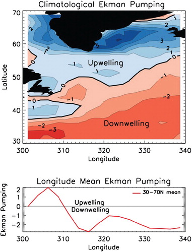
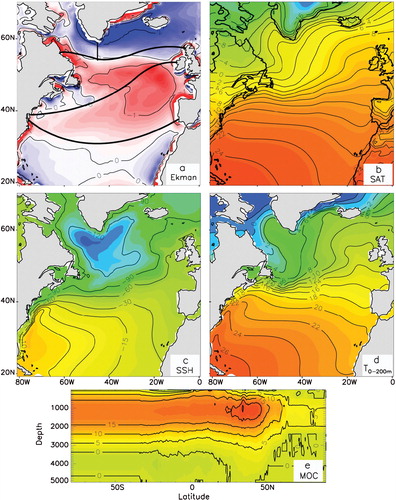
Wind observations were obtained from the National Centers for Environmental Prediction/National Center for Atmospheric Research (NCEP/NCAR) reanalysis 2.5×2.5 gridded daily dataset from 1948 to the present (http://www.esrl.noaa.gov/psd/data/gridded/data.ncep.reanalysis.surface.html, Kalnay et al., 1996). Time series of wind stress were used to estimate Ekman pumping velocity, w _e , over the basin. The estimates of w _e were averaged in time at all domain grid points and the resulting pattern is displayed in the top panel of Fig. 2, while the bottom panel displays average w _e values over each longitude of the basin (the latter are used in stochastic external forcing to force the model). Positive (negative) values represent cyclonic (anti-cyclonic) wind stress exerted on the surface causing a confluence (diffluence) of surface waters resulting in upwelling (downwelling) processes.

Fig. 2.  Climatological Ekman pumping velocity (1948–2008). (Top) Climatological Ekman pumping velocity (10⁻⁶ m s⁻¹) over the North Atlantic Ocean derived from the NCEP Reanalysis winds at 10 m height. (Bottom) Mean climatological Ekman pumping velocity (10⁻⁶ m s⁻¹) averaged over each longitude belt of the basin.

Two observational parameters, SAT and w _e , were then used to develop external stochastic forcings (F _T in eq. 8 and F _τ in eq. 11, respectively) in order to generate a synthetic set of stochastic time series that captured important statistical properties of actual observations. Prior to statistical analyses, these two time series were detrended using trends evaluated by the least-squares best-fit method. For each stochastic time series, a range of fluctuations was defined by observation-based SDs whereas persistence of processes was incorporated into stochastic forcing via the Hurst exponent, H, estimation (Hurst, 1951).

H provides a quantification of long-range correlations within a time series across multiple time scales. Values for H range between 0 and 1 with H = 0.5 indicating short-range memory processes, 0.0 < H<0.5 indicating an anti-persistent pattern and 0.5 < H<1.0 indicating a persistent pattern associated with a slow decay of correlation function. For example, Stephenson et al. (2000) found slow memory in time series of the NAO index. Particularly, they showed that for the low-frequency band the spectral density is approximated by the power law of P(ω) ≈ ω ^−2d where d = H–0.5=0.13 and, therefore, the NAO index H is ~0.60–0.65.

We note that not only quantitative estimates of slow memory but also the existence of slow memory in climatic time series is often questionable. Barbosa et al. (2006) used discrete wavelet analysis to study slow memory of the NAO index which was defined by using two slightly different ways: one index was defined by using SLP time series from Gibraltar and the other one was defined using SLP record from nearby Lisbon. They found that the persistence varied substantially depending of the geographical location chosen to define the NAO. Despite these uncertainties, we consider NAO-related external forcing as a process with slow memory because such a forcing may (we hypothesise) accentuate the NA multidecadal variability.

We estimated H using the Rescaled Range (R/S) method (Mandelbrot and Wallis, 1969) for each observational time series used in the definition of stochastic forcing, resulting in a value of H = 0.88 for the monthly SAT anomalies time series. High H signifies long-term correlations in this observational time series. The Hurst exponent for SAT and winds describes the self-similarity across all time scales. The Ekman pumping time series was handled slightly differently. Hurst exponents using monthly Ekman pumping were determined for each grid cell and were found to be quite uniform, varying spatially in magnitude by only 0.03. The H can vary with time scale and for annual Ekman pumping had two clear regimes, above and below ~1 yr. In our study, we used H = 0.60 that applies to the interannual and longer time scales and indicates weak persistence. This estimate is very close to results of Stephenson et al. (2000). In contrast, the shorter time scale Hurst exponent was more strongly persistent (we note, however, that this persistence may be due to existence of annual cycle).

Next, 500-year synthetic time series were generated for the SAT and w _e using observation-based SDs and H. Synthetic time series have been constructed using the method developed by Mandelbrot as explained by Feder (see Section 9.6 in Feder, 1988) involving a Gaussian random walk process with time correlations. In this process, the fractional Brownian motion is characterised by a time series in which the increments come from a normal distribution of given variance where subsequent values are correlated with previous values with a given memory length (i.e. dependence, or correlation, with previous values). This allows the generation of surrogate time series of given H, which describes the correlation of that memory. Each synthetic time series was normalised by its SD and then multiplied by corresponding observation-based SD.

Model experiments were executed separately with the synthetic forcing and a random white noise forcing for comparison. Synthetic external forcing for the white noise experiments was generated following the same approach used for H-based synthetic time series with the exception that the synthetic H-based time series were replaced by a random seed time series. A series of experiments utilising the box model and external stochastic forcings were developed in order to evaluate the relative role of various forcings and various terms in the model. Additionally, a set of experiments was carried out incorporating a white noise external forcing.

4. Analysis of simple model results

4.1. Spectra

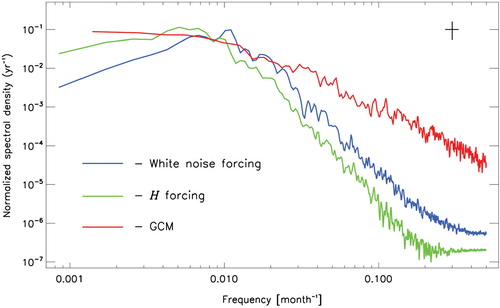
In this section, the results of our model experiments are presented and discussed. The time series of the oceanic responses are shown in Fig. 3. In all of the experiments, the model responses resulted in redder spectra compared with spectra of the forcing. This is true for the model excited by white noise forcing and ‘realistic’ H-based forcing (not shown). This result arises from the fundamental property of oceanic baroclinic response to external stochastic (white noise) excitation, which, as Frankignoul et al. (1997) demonstrated analytically, results in reddening of the spectra. Spectral slopes in our model for the high-frequency band are equal to approximately −3.6 for the white noise forcing and −4.2 for the H forcing. We also see a maximum of spectra at the low-frequency band and rapid power decrease towards the higher frequencies; we discuss the high-frequency slope and low-frequency spectral maximum later, in the section devoted to sensitivity of the solutions to the choice of the model parameters (Appendix A.1.). We note also that, quite naturally, our analysis demonstrates redder spectra of the oceanic response to H-based external forcing compared with oceanic response to white noise excitation (Fig. 4). These results are in general agreement with theory and observations (e.g. Hasselmann, 1976; Frankignoul and Hasselmann, 1977; Battisti et al., 1995; Frankignoul et al., 1997, Neelin and Weng, 1999; Marshall et al., 2001).

Fig. 3.  Simulated time series of ocean temperature response (°C, 3d panel), vertical MOC (blue) and horizontal gyre (red) anomalies (Sv, 4th panel) forced by synthetic forcing including SAT forcing (°C, 1st panel) and Wind forcing (Sv, 2d panel). Note that daily time series of synthetic forcings are shown by dashed lines and 7 yr running mean time series of these forcings are shown by solid lines. Note also that the MOC anomalies are shown using a reverse scale. A striking similarity is apparent between the Wind forcing (2d panel) and MOC and Gyre responses (4th panel).

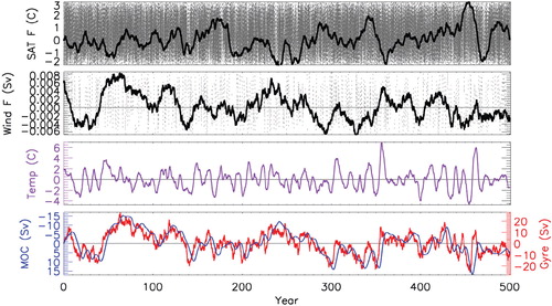
Fig. 4.  Power spectra of water temperature anomalies for experiments with synthetic H-based and white noise wind forcing. For comparison purposes, spectra from GCM CCM4 simulations are also shown. Vertical bar at 0.3 mo⁻¹ frequency show 95% confidence interval.

We also note practically identical spectral transfer functions, one of which links spectra of external forcing and the baroclinic system response as shown by Frankignoul et al. (1997), their eq. 16), and another describes the effect of the running mean smoothing operation (Munk, 1960). This can explain the strong correspondence between the smoothed synthetic wind stress curl forcing and the simulated horizontal (Gyre) and vertical (MOC) oceanic circulation responses (Fig. 3). The correlation between the wind stress curl forcing and resulting Gyre anomalies was R = 0.51 with a lag of ~1 yr, while the anti-correlation with the resulting MOC anomalies was R = −0.47 with a lag of ~4 yr (all correlations discussed in the text are statistically significant at 95% level unless stated otherwise). This finding suggests that the simulated ocean response was a reaction of the system to the cumulative effect of atmospheric forcing averaged over a limited time window; the width of the window is defined by damping properties of the system. This result agrees well with the theoretical findings of Hasselmann (1976) who found that ‘slow changes of climate are explained as the integral response to continuous random excitation by short period “weather” disturbances’. Caution should however be exercised in the determination of a specific time frame since it may vary dependent upon the non-dimensional scaling factors utilised in the model.

4.2. Multidecadal variability

The simulated time series demonstrate signs of multidecadal variability in both atmospheric forcing and the oceanic response (Fig. 3). However, it is still unclear whether the ocean or atmosphere is the dominant forcing owing to the complexity of the interactions within the system. For example, the atmosphere may imprint upon the ocean surface, but the atmospheric conditions are also modified by the underlying ocean. Probably, our results may be better understood in terms of a positive feedback mechanism in which multidecadal variability induced by ocean and air–sea interactions is projected on changes in the atmosphere enhancing further oceanic multidecadal fluctuations.

The simple model results demonstrated the dominance of the wind stress curl forcing over SAT forcing. The simulated model responses suggest that the wind forcing is important in driving changes of NA upper ocean temperature anomalies as well as the intensity of both the horizontal and vertical cells of the ocean circulation. This is corroborated by the high correlation between the ocean response and wind forcing and much lower correlation of simulated ocean variability and SAT forcing. However, the model design affects the simulated system response to different external forcings so the simple model results should be interpreted with caution. At the same time, these results are corroborated by analysis of GCM-based results (Section 5) which showed the strongest cross-correlation between the simulated atmospheric forcing and oceanic response for wind stress curl (R=−0.56 between Ψ _g and Ekman pumping velocity; compare with R=−0.25 between Ψ _g and SAT). We note that a suite of sensitivity experiments, where the model was forced by each external forcing individually, corroborated that wind stresses are the key forcing for simulated NA variability. A high correlation was found between the simulated variables in the most-complete and the wind-only forcing experiments (not shown, see Legatt, 2010 for details). At the same time, the oceanic variability excited by atmospheric heat fluxes is also important. For example, experiments with the SAT forcing demonstrated that warmer northern NA enhances the NAO heat flux leading to a delayed damping of the ocean temperature anomalies and a negative feedback on both Gyre circulation and MOC.

These experiments also partially address the issue of interdependencies of the external forcings used in the experiments (which all are related to the NAO). For example, the GCM results discussed in the next section in detail show that Ekman pumping and SAT time series are correlated at R = 0.36. However, to better understand the role of these interdependencies requires carefully designed experiments with a coupled atmosphere–ocean model. We will return to the discussion of the role of external forcing (including winds) in the last section of the paper.

4.3. Compensatory mechanism

The anti-correlation found between the intensity of the horizontal Ψ _g and vertical Ψ _m branches of the oceanic circulation (R = −0.97, Ψ _g leads Ψ _m by 2 yr) and lower correlation between the simulated ocean temperature anomalies and each branch of the oceanic circulation (R~0.4) suggests a mechanism in which the horizontal Gyre circulation and vertical MOC circulation act together to compensate for a lack or excess of heat northward transport, thus maintaining the heat balance in the system. On the basis of this analysis, the compensation mechanism can be explained by an initially induced wind forcing on the model, resulting in a strengthened horizontal Gyre circulation cell. Over a period of time this circulation increases the net pole-ward transfer of heat, increasing the average SST over the northern portion of the basin, in turn decreasing the north–south temperature gradient. This weakened temperature gradient results in a weaker vertical MOC circulation, decreasing the net poleward heat transport, which would be compensated for by an enhanced horizontal Gyre circulation increasing net pole-ward heat transport. A conceptually similar mechanism was proposed by Bjerknes (1964), who suggested that atmosphere and ocean work together in order to stabilise northward heat supply in the atmosphere–ocean system and the deficit of heat transport by the atmosphere is compensated for by enhanced oceanic heat transport and vice versa. Marshall et al. (2001) hypothesised that a similar compensation mechanism may exist in the ocean, in which shifts in the phase of the NAO alter horizontal intergyre gyre circulation and the meridional heat transport, which is compensated for by adjustments of heat transport by MOC circulation. The choice of the model parameters in the original Marshall et al. (2001) model assumes out-of-phase responses of Ψ _m and Ψ _g (see Appendix A.1. for details). Thus, both Ψ _m and Ψ _g tend to compensate each other thus reducing temperature change and therefore maintaining the heat balance in the system.

The diagnostic of the simple model responses to external stochastic forces may be summarised as following:

• Anomalously strong westerlies associated with the NAO+ (strong negative Ekman pumping) enhance a clockwise intergyre gyre with a ~1 yr delay (as defined via lagged correlation, R _{lag = 1 yr} =0.51).

• The strong anticyclonic intergyre gyre produces a positive ocean temperature anomaly in the northern NA (R _{lag = 5 yr} =0.37).

• Weaker north–south ocean temperature contrast results in a damped MOC with a time delay of several years (correlation between temperature and Ψ _m anomalies is R _{lag = 3 yr} =0.38).

• Warmer northern NA enhances the heat flux to the atmosphere leading to a delayed damping of the ocean temperature anomalies and a negative feedback on both Gyre circulation and MOC. However, in the present model configuration this feedback mechanism is minor.

• Suppressed MOC leads to a negative feedback forcing a decrease of the oceanic temperatures in the northern box.

4.4. Sensitivity of the solution to the choice of the model parameters: Amplification mechanism

We note that the properties of this simulated oceanic response to the external forcing strongly depend on the choice of the model parameters. For example, for a simplified case (eqs. A1–A3) the model equations can be rewritten in order to get equations for anomalous temperature (eqs. A4 or A5) and each streamfunction (eqs. A6 and A7 and Appendix A.1.). Properties of the ordinary second-order differential equation for temperature anomalies (eq. A5) are well known. They depend on D = λ ²−4(ms+fg). The case D > 0 corresponds to unbounded solution of eq. (A4) (for the case of unforced solution and ms+fg<0; forced solutions will be bounded). If D<0, eq. (A4) describes damped oscillations. Five parameters defining D and used in the simple model (see Table A1) correspond to D = −19.1 < 0 thus providing physically justified solution.

Marshall et al. (2001) provided a comprehensive analysis of sensitivity of the model solutions to parameter values. Particularly, using observational arguments Marshall et al. suggested that setting f<0 and g<0 is difficult to reconcile in the framework of this model.

However, negative f and g were used by Jin (1997) and also in the recent analysis by Schneider and Fan (2012). For example, Schneider and Fan used a simple stochastically forced model of the NA tripole SST variability and found that, in comparison with the Marshall et al. (2001) model, the atmospheric heat flux feedback damps the tripole SST pattern and counterclockwise intergyre gyre enhances the tripole pattern.

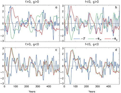
We rerun the model using three additional combinations of signs for the model parameters f and g (in addition to the standard case of positive f and g). Fig. 5 demonstrates that the case with f<0 and g > 0 (panel b) yields low-frequency variations which are very similar to the standard case (panel a). In this case, damping in the system emphasises the role of the external forcing leading to relatively low sensitivity of the solution to the choice of f. In the case of g<0 the physical interpretation of the solution should differ from that provided by Marshall et al. (2001), a possible implementation of such a model may be similar to the one used by Schneider and Fan (2012). Because in the case of g<0 both streamfunctions Ψ _g and Ψ _m work together maintaining the heat balance in the system and each streamfunction amplifies the effect of its counterpart, we will call this an amplification mechanism. Detailed analysis of this mechanism is provided in Appendix A.1.

Fig. 5.  Simulated 15-year running mean smoothed time series of ocean temperature T, vertical MOC Ψ _m and horizontal gyre Ψ _g anomalies forced by synthetic forcing for four combinations of signs of the model parameters f and g. All time series are normalised by their SDs in order to fit the same vertical scale.

5. Compensatory and amplification mechanisms in general circulation model

The major emphasis of this study comprises an analysis of simple model results but is augmented with a GCM analysis that focuses on the NA response to atmospheric forcing. For this purpose, we used 300 yr of a control model run from fully coupled global climate model CCSM4. This model simulation is conducted in preparation for the new Intergovernmental Panel on Climate Change (IPCC) Fifth Assessment Report. Detailed information about the model and its simulation design can be found in Gent et al. (2011). In this section, GCM data are used to gain insight about governing forces driving air–sea interactions in the NA hypothesised from the analysis of our simple model results described in Section 4 and test the existence of this relationship between the gyre circulation and the MOC in a more complete model. Specifically, we use GCM results to gain a better understanding of the compensatory mechanism found in the simple model. The readily available GCM data are a good tool for such an analysis. CCSM4 is a state-of-the-art GCM that we have had experience with in the past analysing simulation results from the previous version of the model (e.g. Polyakov et al., 2010). Note that the objectives of this analysis are somewhat restricted – we do not attempt to explore physical mechanisms in-depth, which would require performing a suite of model sensitivity simulations but rather we use the available simulation to determine what types of responses are possible in the model.

The model was successful in simulating the major features of the NA SAT, upper 200 m ocean potential temperature, SSH and MOC (Fig. 6). For example, the spatial patterns of SAT and upper 200 m potential water temperature, in which zonal distribution is modulated by the oceanic surface circulation, are in reasonable agreement with observations (for comparison, see Woodruff et al. (2011) for SAT and NA climatology from the World Ocean Database 2005 (Boyer et al., 2006) for water temperature). We note, however, that the simulated temperatures are somewhat cooler compared with what the observational climatologies provide. That is why for our analysis of Gulf Stream north–south displacements SST 8°C isotherm is used as a measure of position of the Gulf Stream core. The simulated SSH captures well the spatial SSH pattern derived from observations with a depression centred over the subpolar gyre and sea-level elevation associated with the tropical gyre (compare Fig. 6c with Fig. 1 from Niiler et al., 2003). The model demonstrates reasonably good skills in simulating the Atlantic MOC (Fig. 6e, see also Danabasoglu et al., 2012 for details); the intensity of the MOC used in our analysis is sampled at 40°N thus crossing the simulated MOC core. The model was somewhat less skilful in reproducing the spatial distribution of the Ekman pumping velocity with a northward shift of the zero wind stress curl line (compare Fig. 6a with simulated and Fig. 2 with observed Ekman pumping velocity associated with NAO + ). This is probably due to the exaggerated tongue of the simulated positive anomaly penetrating the Labrador Sea (the hint of which is also seen in the observed distribution). This northward shift of the zero wind stress curl line explains our choice for the position of the section (Fig. 6a) for calculating of the gyre streamfunction anomalies Ψ _g . The simulated zero curl line was also used to define the lower boundary of the domain for calculation of water temperature time series (the upper boundary was defined by 60°N latitude).

Fig. 6.  Simulated CCSM4-based North Atlantic horizontal distributions of (a) Ekman pumping velocity (10⁻⁶ m s⁻¹) associated with NAO+, (b) surface air temperature (SAT, °C), (c) sea-surface height (SSH, cm) and (d) potential water temperature averaged within the upper 200 m layer (T_{0–200 m}, °C) and (e) vertical cross-section of the meridional overturning circulation (MOC, Sv). In addition, panel (a) shows the location of cross-section (black line segment southward of Greenland) used for diagnostics of simulated water transports shown in Fig. 7. For comparison, panel (a) shows a Z-like pattern of observation-based wind stress curl from Marshall et al. (2001) also shown in Fig. 1 and used in defining the simple model domain.

The smoothed time series of anomalous SAT, Ekman pumping velocity, gyre and MOC streamfunctions, water temperature and NAO index (defined as SLP difference between the Icelandic low and Azores high) derived from the CCSM4 control run are shown in Fig. 7. Variability expressed by these time series is dominated by long-term (multidecadal) fluctuations. We note, however, that the amplitude of variations simulated by the GCM and the simple model differ substantially (Figs. 3 and 7). There are also some differences in power spectra between the GCM and simple model (the box-like model shows somewhat redder spectra and a peak at low frequencies, Fig. 4). In this study, we have not explored important physical mechanisms like convective ventilation (e.g. Hawkins and Sutton, 2007), air–sea interactions (e.g. Bhatt et al., 1998; Timmermann et al., 1998) or internal oceanic thermohaline circulation (e.g. Vellinga and Wu, 2004) driving this variability in this GCM. However, the GCM modelling results provide general support for some of our simple model conclusions. For example, the CCSM4 results demonstrate the dependence of the simulated oceanic variability on NAO (Fig. 7, correlation between Ψ _g and model NAO was R = 0.26).

Fig. 7.  Simulated 7 yr running mean CCSM4-based time series of (a) SAT (°C) anomalies, (b) anomalies of Ekman pumping velocity (10⁻⁶ m s⁻¹), (c) anomalous intergyre gyre streamfunction Ψ _g (Sv) and its components: barotropic component based on sea level tilt , steric component and baroclinic component , (d) anomalous gyre Ψ _g and MOC Ψ _m streamfunctions (Sv) and NAO (normalised by 5 in order to match the scale) and (e) water temperature anomalies (°C) averaged over the upper 200 m layer limited by 60°N from the top and by the simulated zero wind stress curl line from the bottom and NAO (normalised by 10). SAT and Ekman pumping velocity anomalies are averaged over the triangle limited by 60°N latitude, 80°W longitude and zero wind stress curl line. Streamfunctions are computed for the cross-section shown by black line segment in Fig. 6a. Note that the MOC anomalies in panel (d) are shown using a reverse scale.

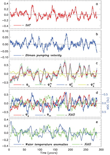
The GCM results corroborate the existence of the amplification mechanism found in the simple model response to atmospheric forcing with the parameter g<0. For example, the GCM-based Ψ _m and Ψ _g are positively correlated (R = 0.47) at zero lag. This result is consistent with the Schneider and Fan (2012) findings. We note, however, that this positive correlation was found between the unsmoothed time series; filtering out high-frequency variability results in close-to-zero correlation at zero lag. Thus, the GCM amplification mechanism is due to high-frequency fluctuations.

Using smoothed time series of Ψ _m and Ψ _g (Fig. 7), we found a negative correlation of R = −0.33 at 7 yr lag (Ψ _g leads). This GCM result is suggestive of the compensatory mechanism found in the simple model response to atmospheric forcing. We must emphasise, however, that this negative correlation should be viewed with great caution. Firstly, autocorrelation in each original time series Ψ _m and Ψ _g reduces the effective length of each time series used for the cross-correlation analysis. Secondly (and more importantly), 7 yr running mean smoothing of a monthly 300 yr long-time series greatly reduces the effective length of the time series [by a factor of O(30–40)] making the estimate statistically insignificant. Thus, we would carefully interpret this result such that the GCM provides a hint for the existence of the compensatory mechanism in the simulated low-frequency fluctuations.

The simulated time series of components of the anomalous gyre streamfunction Ψ _g shown in Fig. 7c suggest that changes of Ψ _g are dominated by variations of sea-level tilt (i.e. by geostrophic component of the streamfunction ) and direct contribution of baroclinic changes defined by the streamfunction component is not significant. However, density-related processes defined by steric sea-level changes and expressed via a streamfunction govern changes in . That is why, we argue, effects of water temperature and salinity changes in CCSM4 are important in shaping the horizontal gyre circulation thus justifying the use of the baroclinic Rossby wave eq. (5) in the Marshall et al. (2001) simple box model.

Concluding this section, we note that the GCM results support the simple-model findings of the importance of wind in regulating the intensity of the Gyre circulation and of the amplification mechanism in which the high-resolution horizontal Gyre circulation and vertical MOC circulation act together maintaining the heat balance in the system. The GCM provides some hint on the existence of the compensatory mechanism; however, we should note that additional experiments targeting the complex interactions in the ocean interacting with the atmosphere are necessary to further justify this finding.

6. Concluding remarks and discussion

This investigation of the NA variability utilising a simple stochastically forced model provides a means for discerning the feedbacks and mechanisms impacting variability in the basin. While the model may be simple, it provides useful insights into the mechanisms driving complex variability in Earth's climate and its applications are critical for understanding the complex results of the modern GCMs.

Following the discussion in the previous sections, the major findings are summarised as follows:

• The simulated response of the upper North Atlantic Ocean to atmospheric forcing using the simple model results in model solutions with redder spectra than the spectra of atmospheric forcing. This fact implies that the ocean acts as a low-pass filter utilising the lower-frequency part of the forcing.

• The simulated oceanic dynamical response may be viewed as a cumulative effect of atmospheric forcing over limited time; the length of the time interval is defined by the damping properties of the system.

• An anti-correlation between the simulated intensity of horizontal (Gyre, Ψ _g ) and vertical (MOC, Ψ _m ) circulation cells with the choice of the model parameter g > 0 suggests a compensatory mechanism, in which heat balance in the system is maintained via communication between these two dynamic system components. For instance, an increase of heat supplied by an anomalously strong gyre circulation would be balanced by a decrease of heat provided by a weaker MOC circulation and vice versa.

• When the parameter g<0, the model demonstrates a positive correlation between the two circulation branches Ψ _m and Ψ _g suggesting an amplification mechanism in which both vertical and horizontal circulation cells maintain the heat budget in the system compensating its damping properties.

While the first two points are not particularly new (see references and discussion in the text), our experiments with the model add the effect of a non-white noise forcing to the well-known behaviour of the stochastic climate model and quantify the extent to which it makes the spectrum even ‘redder’. We have found signs of multidecadal ocean–atmosphere interactions within our simple modelling experiments. This variability in the model was excited by a long-term component hidden in the external forcing (wind stress curl), which is new for stochastically forced box-like models. On the basis of these findings we argue that these results may be better understood in terms of a positive feedback mechanism in which multidecadal variability induced by ocean and air–sea interactions is projected on changes in the atmosphere enhancing further oceanic multidecadal fluctuations.

The compensation and amplification mechanisms found in the simple model and also in GCM results are a key, new and intriguing result providing an important perspective on air–sea interactions in the NA. The utility of investigating a very simple box-like model along with a GCM is demonstrated by better understanding of both simple model and GCM results as well as their limitations. Thus, while the model is very simple (see discussion of its limitations in Marshall et al. (2001) and in the following discussion), it produces meaningful and useful results.

The Marshall et al. (2001) theory suggested that decadal-scale Rossby wave adjustment to wind stress changes related to the NAO causes oscillatory behaviour in the intergyre gyre governed by north–south heat transports by anomalous currents. In our experiments with the simple box-like model proposed by Marshall et al. (2001), we found compensatory and amplification mechanisms between the horizontal gyre and vertical MOC circulation which both work hand-in-hand in order to maintain the heat balance within the system. Given the simplicity of the model, the finding of the compensatory and amplification mechanisms is intriguing and is corroborated in general terms by results of numerical simulations using the state-of-the-art global GCM (we reiterate here that further analysis is necessary to provide statistically sound evidence for the GCM-derived compensatory mechanism). In this, the simple model provided guidance to the analysis of the GCM results, thus emphasising the important role simple, box-like models may play in interpreting simulations provided by complex modern climate models.

The model results are sensitive to the choice of the model parameters. The level of uncertainty is emphasised by the on-going debate on the sign of several dynamically important model parameters (for details, see Marshall et al., 2001 and recent overview by Schneider and Fan, 2012). In this discussion, observational and GCM-based arguments are used. As we demonstrated, physical mechanisms governing simulated NA variability may be fundamentally different depending on the sign of g. For example, Marshall et al. (2001) found that clockwise intergyre gyre causes a positive SST tendency (i.e. g > 0), whereas Schneider and Fan (2012) results demonstrated the opposite feedback when counterclockwise intergyre gyre governs a positive SST tripole tendency (i.e. g<0); the earlier Eden and Greatbatch (2003) modelling study demonstrated a feedback mechanism similar to Schneider and Fan's. Thus, we argue that at this stage, either choice of sign of dynamically important model parameters affecting mechanisms associated with the simulated NA variability should not be ruled out.

Perhaps, one of the most significant omissions in the simple stochastically driven model is that of the fast wind-driven barotropic adjustment of the oceanic circulation to wind forcing. The GCM used in this study suggests a co-existence of a slow baroclinic adjustment (via the compensatory mechanism) with a fast oceanic response to wind forcing (via the amplification mechanism). A modelling study by Eden and Willebrand (2001) also demonstrated the co-existence of two time scales. One scale is related to fast oceanic response to wind in the form of (for NAO + ) anomalous anticyclonic barotropic circulation near the subpolar front associated with decreased northward heat transport and increase northward heat transport in the subtropics. The second (slow) scale is associated with increased subpolar heat transport due to intensified MOC and subpolar gyre. Deshayes and Frankignoul (2008) provided further support to this concept: using modelling results they demonstrated that variability of the subpolar gyre circulation and MOC is governed by fast barotropic adjustment to NAO-related Ekman pumping anomalies, whereas slow interdecadal-to-decadal variability is caused by the baroclinic adjustment to Ekman pumping, buoyancy forcing and dense water formation.

This discussion suggests that the simple stochastically forced ocean model used in our study may be enriched by inclusion of the barotropic circulation interrelated to changes of the oceanic temperature and baroclinic circulation. This may also have an impact on the balance of external forces affecting the simulated NA variability. However, the inclusion of the barotropic circulation in the simple model may not be a trivial task because the barotropic circulation strongly depends on density changes (see Fig. 7c) so that the barotropic and baroclinic factors may be coupled via a complex, probably, non-linear relationship.

We also note that the Eden and Greatbatch (2003) modelling results suggest that the Rossby wave adjustment may not be important in shaping NA decadal variations; instead they argue that anomalous geostrophic advection plays an important role in sustaining variability. However, extensive analysis carried out by Frankignoul et al. (1997) demonstrated the utility of the Rossby wave model via a broad consistency found between the predicted power spectra of the baroclinic pressure and the observed spectrum of sea level change and temperature fluctuations and GCM-based spectra of NA pressure variability. Thus, we argue that the Rossby wave eq. (5) (with its limitations and caveats) is a useful and powerful instrument for the simulation of important features of the NA variability.

In conclusion, we note that despite the simple model limitations and uncertainties related to the choice of the model parameters, it was instrumental in identifying the compensatory and amplification mechanisms in the simple model and complex GCM simulations. We stress the importance of continuing to investigate the mechanisms driving NA variability, as these climate variability patterns are of great importance to sustaining the global transport of heat in the ocean through the thermohaline circulation and of potential use in decadal and longer climate predictability.

Acknowledgements

We thank David Newman for help with the synthetic time series generation and the R/S analysis, John Marshall for useful consultation and Andrey Pnyushkov for help with spectral analysis. We thank two anonymous reviewers for helping to improve the manuscript. This study was supported by JAMSTEC (RL, IP, XZ), NASA grant NA06OAR4600183 (IP, UB), DOE grant DE-SC0001898 (UB, IP) and Russian Foundation for Fundamental Research grant #11-05-00734-a (RB). R. Legatt was supported by a graduate fellowship from the College of Natural Science and Mathematics and the Graduate School at University of Alaska Fairbanks.

8. Appendix

A.1. Analysis of a simple climate model

Let us start with non-dimensional model equations neglecting spatial variations of Ψ _g and all external forcings but wind:A1 A2 A3

Table A1. Values of non-dimensional (except H_ek) factors used in model equations

Non-dimensional factor	Description	Value
	Factor describing efficiency of heat transport by MOC	16.82
	Factor describing efficiency of heat transport by ocean gyre	8.41
λ = d−fe	Factor describing intensity of damping of ocean temperature anomalies by air–sea interactions and wind effects	1.04
s = S·Y·t delay	Solenoidal factor driving meridional overturning	0.2
	Damping coefficient for ocean temperature anomalies	2.35
	Positive factor describing feedback of wind effects on ocean temperature anomalies	1.64
f	Factor for feedback of ocean temperature anomalies on wind stress	0.2
	Pseudo air–sea heat flux by Ekman heat transport [kg s^−3]	13.95

where F is external Ekman pumping forcing. Equations (A1–A3) can be rewritten in order to get an equation for anomalous temperature by excluding anomalies of streamfunctions:A4

can be rewritten in a more compact way using the following definitions: , , and . Then we haveA5

and eqs. (A2) and (A3) becomeA6 A7

Equation (A5) may be solved analytically, and solutions for various combinations of parameters a and b may be found in the study of Kamke (1948), see expressions 2.35 and 2.36 from this book). These solutions may be generally described using combinations of forced and free oscillations.

A.1.1. Solution for periodic external forcing.

In the model, the parameter a>0, therefore free oscillations decay exponentially except when and b<0. Let us consider eq. (A5) with periodic external forcingA8

For this forcing, the solution of eq. (A5) yieldsA9

whereA10

In some cases it is more convenient to express the solution using amplitude and phase :A11

whereA12

Solutions for eqs. (A6–A7) for Ψ _m and Ψ _g are given byA13 A14

Using amplitude and phase notation, let us rewrite eqs. (A13) and (A14): A15 A16

and obtain expressions for phases and of the streamfunctionsA17 A18

From expressions (A17 and A18) the phase difference between solutions for Ψ _m and Ψ _g isA19

Because , the latter may be written asA20

It follows from eq. (A20) that the phase difference between Ψ _m and Ψ _g is defined by the frequency of external forcing ω and the product ms. If ω ² >ms then the phase difference is <0.5 π, resulting in positively correlated Ψ _m and Ψ _g ; we call this as amplification mechanism. If ω ²<ms then and the Ψ _m and Ψ _g are negatively correlated, and we relate this case to the compensation mechanism. If ω ² =ms then the oscillations of Ψ _m and Ψ _g are orthogonal and there is no correlation between the solutions for the streamfunctions.

It follows from eqs. (A12) and (A17) thatA21

which corresponds to a 0.5 π phase shift between the anomalous temperature and Ψ _m (streamfunction leads).

Note that if m = 0, then the system of eqs. (A1–A3) is reduced to the system of eqs. (A1) and (A2) for T and Ψ _g and eq. (A3) for Ψ _m . If s = 0, then the system of eqs. (A1–A3) is also reduced to (A1–A2), because Ψ _m becomes constant: Ψ _m (t)=Ψ _m (0).

Let us now describe the amplitudes of the streamfuncTions and ,A22

where A23

where .

Simplification yieldsA24

Both streamfunctions have the same asymptotes for the low-frequency band: and for . This means that the transfer functions cannot be intergrated over frequency. Variabce of both streamfunctions becomes unbounded in time, which is characteristic of a non-stationary process.

Finally, we note that the ratio of streamfunction amplitudes may be defined asA25

asA26

and allows an easy estimate of relative contribution of each streamfunction.

A.1.2. Correlations between the streamfunctions for a periodic external forcing.

Let us define formally the correlation coefficient R(ω) between Ψ _m and Ψ _g asA27

where and define means. Because both functions are periodic with periods defined as , we can integrate eq. (A27) from 0 to which yieldsA28

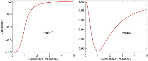
Equation (A28) demonstrates that when , R(ω) is negative and vice versa. Besides, when , and when . Thus, R(ω) asymptotically approaches either 1 (when ms<0) or –1 (when ms > 0). Fig. 8 shows R(ω) as a function of ω illustrating both possible scenarious. These results corroborate conclusions from the previous section that the realisation of compensatory or amplification regime depends on the value of ms.

Fig. 8.  Correlation coefficient R(ω) derived from eq. A42 as a function of ω for (left) ms=1 and (right) ms=−1.

A.1.3. Spectral properties of the system under stochastic external forcing.

Let us now consider the case when the function in eq. (A5) is a stationary stochastic process, with a spectral density . In this case, the spectral density of the process is described by the following expression (e.g. Yaglom, 1981):A29

where is the transfer function of the linear stochastic process andA30

Note that expressions from the right-hand sides of eqs. (A30) and (A12) for amplitude are identical. Asymptotic behaviour in the high-frequency band is different from standard Langevin and characterised by S(ω)~ω⁻⁴.

Let us consider extrema of the transfer function , differentiating it over ω and equating it to zero:A31

Two extrema are located at and . When , the second derivative of is . Therefore is associated with a local minimum of when and with a local maximum when . The second point of the extremum exists when only. The second derivative of in this case is . At this point it is negative, and the transfer function has a maximum.

Note that at , the transfer function is defines as and does not depend on the damping properties of the system defines by a and when .

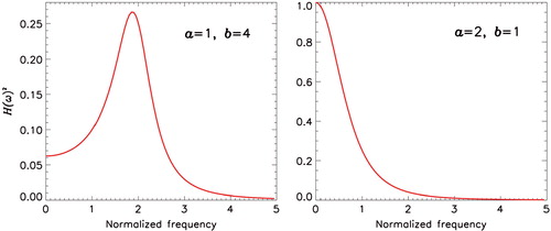
Figure 9 shows examples of for two cases when and . The solutions for the two cases are qualitatively different. For , eq. (A5) has maximal at low frequencies, peaking at . For the case , peaks at the frequency defined by . Correspondingly, the spectral density of water temperature has a maximum at the same frequency. Thus, multidecadal variability excited in the ocean by high-frequency weather «noise» may contribute significantly to the total variance of the climate system. With the selected set of the model parameters, multidecadal variability looks quasi-periodic, however, strictly speaking, is not periodic.

Fig. 9.  Transfer function derived from eq. A45 for (left) a = 1 and b = 4 which correspond to the case and for (right) a = 2 and b = 1 which correspond to the case.

We note that even though the solution for eq. (A5) under impact of external random stationary forcing X(t) is stationary, the solution of the system of eqs. (A5–A7) is not necessarily stationary. For example, let us consider two streamfunctions  Ψ _m  and  Ψ _g , and introduce a new variable, W:A32

It is evident thatA33

Dynamics of the linear equation for W are defined by external forcing F(t) only and does not depend on temperature anomalies T. There is no dissipation term in eq. (A33), therefore when X(t) is a random stationary process, the variable W is a stochastic integral of the right-hand part of eq. (A33). Such an integral is, by definition, a non-stationary function, whose variance is unbound and increases in time: . Thus, it follows from eq. (A32), that solutions for Ψ _m and Ψ _g are also unbound. However, because the solution of eq. (A5) for T is limited ( when ), then we may write an approximate relationshipA34

which suggests negative correlation between the components of the streamfunction. However, such a correlation, as well as the non-stationary behaviour of the two streamfunctions, is caused by oversimplification of the model. In the original system of eqs. (8–11), damping of unrealistic, physically unjustified solutions is carried out via the boundary condition for Ψ _g . Non-stationarity in the solution can be avoided; however, if dissipative terms are incorporated in eqs. (A6 and A7) for both streamfunctions so that the system of equations becomesA35 A36 A37

Equations (A36) and (A37) are of the Langevin type; therefore, the solutions for the streamfunctions are stochastic stationary processes. Even though the relationship between phases for each streamfunction now depends on dissipative parameter , it is easy to show that the phase difference between Ψ _m and Ψ _g is expressed by the same expression (A20), derived for a non-dissipative system. This is also true for the correlation between Ψ _m and Ψ _g which is expressed by the relationship (A28).

References

- Barbosa S. Silva M. E. Fernandes M. J. Wavelet analysis of the Lisbon and Gibraltar North Atlantic Oscillation winter indices. Int. J. Climatol. 2006; 26: 581–593. 10.3402/tellusa.v64i0.18695.
- Barnett, T. P, Pierce, D. W, AchutaRao, K. M, Gleckler, P. J, Santer, B. D and co-authors. 2005. Penetration of human-induced warming into the world's oceans. Science. 309, 284–287. 10.3402/tellusa.v64i0.18695.
- Barsugli J. J. Battisti D. S. The basic effects of atmosphere–ocean thermal coupling on middle-latitude variability. J. Atmos. Sci. 1998; 55: 477–493. 10.3402/tellusa.v64i0.18695.
- Battisti D. S. Bhatt U. S. Alexander M. A. A modeling study of the interannual variability in the North Atlantic Ocean. J. Clim. 1995; 8: 3067–3083. 10.3402/tellusa.v64i0.18695.
- Bhatt U. S. Alexander M. A. Battisti D. S. Houghton D. D. Keller L. M. Atmosphere-ocean interaction in the North Atlantic: near surface climate variability. J. Clim. 1998; 11: 1615–1632. 10.3402/tellusa.v64i0.18695.
- Bjerknes, J. 1964. Atlantic air–sea interaction. In: Advances in Geophysics. H. E. Landberg and J. van Mieghem, vol. 10, Academic Press: New York, pp. 1–8.
- Boyer, T. P, Antonov, J. I, Baranova, O. K, Garcia, H, Johnson, D. R and co-authors. 2006. World Ocean Database 2005. In: NOAA Atlas NESDIS 60. S. Levitus, U.S. Government Printing Office: WashingtonDC, 190. pp.
- Cessi P. Thermal feedback on wind stress as a contributing cause of climate variability. J. Clim. 2000; 13: 232–244. 10.3402/tellusa.v64i0.18695.
- Curry R. G. Dickson R. R. Yashayaev I. A change in the freshwater balance of the Atlantic Ocean over the past four decades. Nature. 2003; 426: 826–829. 10.3402/tellusa.v64i0.18695.
- Curry R. G. McCartney M. S. Ocean gyre circulation changes associated with the North Atlantic Oscillation. J. Phys. Oceanogr. 2001; 31: 3374–3400. 10.3402/tellusa.v64i0.18695.
- Curry R. G. McCartney M. S. Joyce T. M. Oceanic transport of subpolar climate signals to mid-depth subtropical waters. Nature. 1998; 391: 575–577. 10.3402/tellusa.v64i0.18695.
- Czaja A. Frankignoul C. Influence of the North Atlantic SST anomalies on the atmospheric circulation. Geophys. Res. Lett. 1999; 26: 2969–2972. 10.3402/tellusa.v64i0.18695.
- Danabasoglu G. On multidecadal variability of the Atlantic meridional overturning circulation in the Community Climate System Model Version 3. J. Clim. 2008; 21: 5524–5544. 10.3402/tellusa.v64i0.18695.
- Danabasoglu, G, Yeager, S. G, Kwon, Y.-O, Tribbia, J. J, Phillips, A and co-authors. 2012. Variability of the Atlantic meridional overturning circulation in CCSM4. in press.
- Delworth T. L. Greatbatch R. J. Multidecadal thermohaline circulation variability driven by atmospheric surface flux forcing. J. Clim. 2000; 13: 1481–1495. 10.3402/tellusa.v64i0.18695.
- Delworth T. L. Manabe S. Stouffer R. J. Interdecadal variations of the thermohaline circulation in a coupled ocean–atmosphere model. J. Clim. 1993; 6: 1993–2011. 10.3402/tellusa.v64i0.18695.
- Deser C. Blackmon M. Surface climate variations over the North Atlantic Ocean during winter: 1900-89. J. Clim. 1993; 6: 1743–1753. 10.3402/tellusa.v64i0.18695.
- Deshayes, J and Frankignoul, C. 2008. Simulated variability of the circulation in the North Atlantic from 1953 to 2003. J. Clim. 21, 4919–4933. 10.3402/tellusa.v64i0.18695.
- Dickson R. R. Lazier J. Meincke J. Rhines P. Swift J. Long-term coordinated changes in the convective activity of the North Atlantic. Prog. Oceanogr. 1996; 38: 241–295. 10.3402/tellusa.v64i0.18695.
- Dickson, R. R, Yashayaev, I, Meincke, J, Turrell, B, Dye, S and co-authors. 2002. Rapid freshening of the deep North Atlantic Ocean over the past four decades. Nature. 416, 832–837. 10.3402/tellusa.v64i0.18695.
- Dong B. Sutton R. T. Mechanism of interdecadal thermohaline circulation variability in a coupled ocean–atmosphere GCM. J. Clim. 2005; 18: 1117–1135. 10.3402/tellusa.v64i0.18695.
- Eden C. Greatbatch R. J. A damped decadal oscillation in the North Atlantic climate system. J. Clim. 2003; 16: 4043–4060. 10.3402/tellusa.v64i0.18695.
- Eden C. Jung T. North Atlantic interdecadal variability: ocean response to the North Atlantic oscillation (1865–1997). J. Clim. 2001; 14: 676–691. 10.3402/tellusa.v64i0.18695.
- Eden C. Willebrand J. Mechanism of interannual to decadal variability on the North Atlantic circulation. J. Clim. 2001; 14: 2266–2280. 10.3402/tellusa.v64i0.18695.
- Feder, J. 1988. Fractals. Plenum Press, New York. 283. p.
- Frankignoul C. Czaja A. L'Heveder B. Air–sea feedback in the North Atlantic and surface boundary conditions for ocean models. J. Clim. 1998; 11: 2310–2324. 10.3402/tellusa.v64i0.18695.
- Frankignoul C. Hasselmann K. Stochastic climate models, Part II: application to sea-surface temperature variability and thermocline variability. Tellus. 1977; 29: 289–305. 10.3402/tellusa.v64i0.18695.
- Frankignoul C. Kestenare E. Observed Atlantic SST anomaly impact on the NAO: an update. J. Clim. 2005; 18: 4089–4094. 10.3402/tellusa.v64i0.18695.
- Frankignoul C. Muller P. Zorita E. A simple model of decadal response of the ocean to stochastic wind forcing. J. PhysOceanogr. 1997; 27: 1533–1546.
- Gent, P. R, Danabasoglu, G, Donner, L. J, Holland, M. M, Hunke, E. C and co-authors. 2011. The community climate system model version 4. J. Clim. in press.
- Griffies S. M. Tziperman E. A linear thermohaline oscillator driven by stochastic atmospheric forcing. J. Clim. 1995; 8: 2440–2453. 10.3402/tellusa.v64i0.18695.
- Häkkinen S. Variability of the simulated meridional heat transport in the North Atlantic for the period 1951-1993. J. Geophys. Res. 1999; 104: 10991–11007. 10.3402/tellusa.v64i0.18695.
- Hall A. Manabe S. Can local linear stochastic theory explain sea surface temperature and salinity variability?. Clim. Dyn. 1997; 13: 167–180. 10.3402/tellusa.v64i0.18695.
- Hasselmann K. Stochastic climate models. Part I: theory. Tellus. 1976; 28: 289–305.
- Hawkins E. Sutton R. Variability of the Atlantic thermohaline circulation described by three-dimensional empirical orthogonal functions. Clim. Dyn. 2007; 29: 745–762. 10.3402/tellusa.v64i0.18695.
- Hurrell, J. W, Kushnir, Y, Visbeck, M and Ottersen, G. 2002. An overview of the North Atlantic Oscillation. In: The North Atlantic Oscillation: Climate Significance and Environmental Impact. J. W. Hurrell, Y. Kushnir, G. Ottersen and M. Visbeck, Geophysical Monograph Series. vol. 134, Washington, DC: AGU, pp. 1–35. doi:10.1029/GM134.
- Hurst H. E. Long-term storage capacity of reservoirs. Trans. Am. Soc. Civil Eng. 1951; 116: 770–808.
- Jin F. F. A theory of interdecadal climate variability of the North Pacific Ocean – atmosphere system. J. Clim. 1997; 10: 324–338.
- Joyce T. M. Deser C. Spall M. A. The relation between decadal variability of subtropical mode water and the North Atlantic Oscillation. J. Clim. 2000; 13: 2550–2569. 10.3402/tellusa.v64i0.18695.
- Jungclaus J. H. Haak H. Latif M. Mikolajewicz U. Arctic North Atlantic interactions and multidecadal variability of the meridional overturning circulation. J. Clim. 2005; 18: 4013–4031. 10.3402/tellusa.v64i0.18695.
- Kalnay, E, Kanamitsu, M, Kistler, R, Collins, W, Deaven, D and co-authors. 1996. The NCEP/NCAR 40-year reanalysis project. Bull. Am. Meteorol. Soc. 77, 437–470. 10.3402/tellusa.v64i0.18695.
- Kamke E. Differentialgleichungen, Losungsme thoden und Losungen3rd edn. New York: Chelsea Publishing Company, 666 p, 1948
- Knight J. R. Allan R. J. Folland C. K. Vellinga M. Mann M. E. A signature of persistent thermohaline circulation cycles in observed climate. Geophys. Res. Lett. 2005; 32: L20708.10.3402/tellusa.v64i0.18695.
- Kushnir Y. Interdecadal variations in North-Atlantic sea-surface temperature and associated atmospheric conditions. J. Clim. 1994; 7: 141–157. 10.3402/tellusa.v64i0.18695.
- Legatt, R. A. 2010. North Atlantic Air-Sea Interactions Driven by Atmospheric and Oceanic Stochastic Forcing in a Simple Box Model. Master Degree Thesis. Fairbanks, AK, University of Alaska Fairbanks, GC190.5.L44.
- Mandelbrot, B. B and Wallis, J. R. 1969. Robustness of the rescaled range R/S in the measurement of noncyclic long run statistical dependence. Water Resour. Res. 5(5), 967–988. 10.3402/tellusa.v64i0.18695.
- Marshall J. Johnson H. Goodman J. Interaction of the North Atlantic Oscillation with ocean circulation. J. Clim. 2001; 14(7): 1399–1421. 10.3402/tellusa.v64i0.18695.
- Msadek R. Frankignoul C. Atlantic multidecadal oceanic variability and its influence on the atmosphere in a climate model. Clim. Dyn. 2009; 33: 45–62. 10.3402/tellusa.v64i0.18695.
- Munk W. H. Smoothing and Persistence. J. Meteorol. 1960; 17: 92–93. 10.3402/tellusa.v64i0.18695.
- Neelin J. D. Weng W. Analytical prototypes for ocean-atmosphere interaction at midlatitudes. Part I: coupled feedbacks as a sea surface temperature dependent stochastic process. J. Clim. 1999; 12(3): 697–721. 10.3402/tellusa.v64i0.18695.
- Niiler, P. P, Maximenko, N. A and McWilliams, J. C. 2003. Dynamically balanced absolute sea level of the global ocean derived from near-surface velocity observations. Geophys. Res. Lett. 30(22), 2164. 10.3402/tellusa.v64i0.18695.
- Polyakov, I. V, Alexeev, V. A, Bhatt, U. S, Polyakova, E. I and Zhang, X. 2010. North Atlantic warming: patterns of long-term trend and multidecadal variability. Clim. Dyn. 34, 439–457. 10.3402/tellusa.v64i0.18695.
- Polyakova E. I. Journel A. Polyakov I. V. Bhatt U. S. Changing relationship between the North Atlantic Oscillation index and key North Atlantic climate parameters. Geophys. Res. Lett. 2006; 33: L03711.10.3402/tellusa.v64i0.18695.
- Rogers J. C. The association between the North-Atlantic Oscillation and the southern oscillation in the Northern Hemisphere. Month. Weath. Rev. 1984; 112: 1999–2015. 10.3402/tellusa.v64i0.18695.
- Saravanan R. McWilliams J. C. Advective ocean–atmosphere interaction: an analytical stochastic model with implications for decadal variability. J. Clim. 1998; 11: 165–188. 10.3402/tellusa.v64i0.18695.
- Schneider, E. K and Fan, M. 2012. Observed decadal North Atlantic tripole SST variability. Part II: diagnosis of mechanisms. J. Atmos. Sci. 69, 51–64. 10.3402/tellusa.v64i0.18695.
- Stephenson D. Pava V. Bojariu R. Is the North Atlantic Oscillation a random walk?. Int. J. Climatol. 2000; 20: 1–18. 10.3402/tellusa.v64i0.18695.
- Timmermann A. Latif M. Voss R. Grotzner A. Northern Hemispheric interdecadal variability: a coupled air-sea mode. J. Clim. 1998; 11: 1906–1931. 10.3402/tellusa.v64i0.18695.
- Vellinga M, Wu P. Low-latitude freshwater influence on centennial variability of the Atlantic thermohaline circulation. J. Clim. 2004; 17: 4498–4511. 10.3402/tellusa.v64i0.18695.
- Visbeck, M, Chassignet, E. P, Curry, R, Delworth, T, Dickson, B and co-authors. 2002. The ocean's response to North Atlantic Oscillation variability. In: The North Atlantic Oscillation: Climatic Significance and Environmental Impact. J. W. Hurrell, Y. Kushnir, G. Ottersen, and M. Visbeck, Geophysical Monograph Series, vol. 134, WashingtonDC: AGU. pp. 113–145.
- Weng W. Neelin J. D. On the role of ocean–atmosphere interaction in middle-latitude interdecadal variability. Geophys. Res. Lett. 1998; 25: 167–170. 10.3402/tellusa.v64i0.18695.
- Woodruff, S. D, Worley, S. J, Lubker, S. J, Ji, Z, Freeman, J. E and co-authors. 2011. ICOADS Release 2.5: Extensions and enhancements to the surface marine meteorological archive. Int. J. Climatol. 31, 951–967. 10.3402/tellusa.v64i0.18695.
- Yaglom, A. M. 1981. Correlation Theory of Stationary Random Functions with Examples from Meteorology. Leningrad: Hydrometeoizdat. 280. p.
- Zhang R. Delworth T. L. Held I. M. Can the Atlantic Ocean drive the observed multidecadal variability in Northern Hemisphere mean temperature?. Geophys. Res. Lett. 2007; 34: L02709.10.3402/tellusa.v64i0.18695.
- Zhu, X and Jungclaus, J. 2008. Interdecadal variability of the meridional overturning circulation as an ocean internal mode. Clim. Dyn. 31(6), 731–741. 10.3402/tellusa.v64i0.18695.