Balanced thermal structure of an intensifying tropical cyclone

ABSTRACT

This study tests the hypothesis that the formation of a virtual potential temperature dipole in a developing tropical cyclone is a balanced response to the growth of an associated mid-level vortex. The dipole is collocated with the vortex and consists of a warm anomaly in the upper troposphere and a cool anomaly in the lower troposphere. An axisymmetric approximation to the observed potential vorticity distribution is inverted subject to non-linear balance for two successive days during the formation of typhoon Nuri in 2008. Good agreement is found between the area-averaged actual and balanced virtual temperature dipoles in these two cases. Furthermore, a strong correlation exists between the degree of bottom-heaviness of convective mass flux profiles and the strength of the balanced virtual potential temperature dipole. Since the dipole is balanced, it cannot be an immediate artefact of the existing convection, but rather is an inherent feature of the developing cyclone. Cloud resolving numerical modelling suggests that the dipole temperature anomaly actually promotes more bottom-heavy convective mass flux profiles, as observed. Such profiles are associated with low-level mass and vorticity convergence via mass continuity and the circulation theorem, resulting in low-level spin-up. The present work thus supports the hypothesis that the low-level spin-up associated with tropical cyclogenesis is made possible by the thermodynamic environment created by a strong mid-level vortex.

• tropical cyclones
• tropical cyclogenesis
• nonlinear balance
• geophysical fluid dynamics

1. Introduction

As a tropical storm forms, it develops values of vorticity many times the local Coriolis parameter. This vorticity distribution tends to adjust over time to a state of balance with the potential temperature field. Given the resulting potential vorticity and surface potential temperature distributions, the balanced potential temperature and flow fields may be diagnosed by an ‘inversion’ process (Hoskins et al., 1985). However, due to the strong vorticity in developing tropical cyclones, geostrophic balance is inapplicable to potential vorticity inversion in these systems. In the two-dimensional, axisymmetric case, the more general gradient balance condition suffices (Thorpe, 1985; Schubert and Alworth, 1987). For the fully three-dimensional case, this must be extended to non-linear balance (Bolin, 1955, 1956; Charney, 1955; Lorenz, 1960; McWilliams, 1985; Davis, 1992; Raymond, 1992, 1994).

The thermodynamic perturbations resulting from adjustment to balance are of particular interest, as small variations in the profiles of potential temperature and mixing ratio have been shown to result in large changes in the vertical profile of the vertical mass flux associated with deep convection (Raymond and Sessions, 2007). These results were obtained using a cloud-resolving model (CRM) run in weak temperature gradient mode (WTG; Sobel and Bretherton, 2000; Sobel et al., 2001; Raymond and Zeng, 2005; Raymond, 2007).

Unlike many CRMs that specify a large-scale vertical velocity and examine the resulting changes in the temperature profile, WTG computes the vertical velocity (called the WTG vertical velocity) needed to drive the CRM-averaged temperature profile to an externally specified profile. This so-called reference profile is taken to be characteristic of the surrounding convective environment. Domain-averaged moisture sources and sinks in the CRM result from vertical advection of the mean moisture by the WTG vertical velocity and entrainment and detrainment of moisture produced by lateral flows linked by mass continuity to the WTG vertical velocity.

In the above WTG simulations, the ambient state of the tropics is assumed to be one of radiative–convective equilibrium (RCE). This assumption is justified by the observation that only about 10% of the energy input into the tropical atmosphere from the sun and the surface is exported to higher latitudes (Peixoto and Oort, 1992); the majority is returned to space via outgoing long-wave radiation. The temperature and moisture anomalies assumed by Raymond and Sessions (2007) are perturbations on the RCE state computed by the CRM.

The mass flux profile for convection with an RCE reference profile in Raymond and Sessions (2007) is very top-heavy, with the maximum mass flux occurring near an elevation of 10 km. Increasing the humidity of the reference profile increases the magnitude of the vertical mass flux without changing the elevation of maximum mass flux. However, imposing a dipolar potential temperature anomaly, with approximately 1 K warmer conditions in the upper troposphere and 1 K cooler conditions in the lower troposphere, results in both an increase in the magnitude of the vertical mass flux and a bottom-heavy mass flux profile, i.e. a lowering of the elevation of maximum flux to near 5 km. Something similar to this appears to be occurring in the numerical simulation of tropical cyclogenesis of Bister and Emanuel (1997). Dipole temperature anomalies of this form are frequently seen in convectively disturbed environments in the tropics, e.g. in easterly waves (Reed and Recker, 1971; Cho and Jenkins, 1987).

Support for this CRM result comes from observations of convection in West Pacific disturbances, some of which intensified into typhoons (Raymond et al., 2011). Systems with dipole temperature anomalies, as discussed above, tended to have bottom-heavy mass flux profiles, whereas top-heavy mass flux profiles were correlated with unperturbed temperature profiles.

Bottom-heavy mass flux profiles are a significant aid to tropical cyclone spin-up because strong low-level convergence follows in this case from mass continuity. Spin-up results because the convergent flow carries vorticity inward, resulting in an increase in circulation at fixed radius. (For a complete analysis of the processes involved in spin-up, see Raymond and López Carrillo, 2011.)

Correlation does not imply causality, and one might imagine that strong convection could itself produce a tropospheric temperature dipole. Convection tends to stabilise the environment in which it occurs, which means that it ought to drive the environment toward a moist adiabat, which implies a tendency toward warmer temperatures aloft and cooler conditions at lower levels, given typical tropical soundings. Evaporation of precipitation reinforces this effect at low levels. In this case it would be erroneous to attribute the mass flux profile of the convection to the thermal structure of the environment, since this thermal structure did not exist prior to the convection.

The counter-argument is based on the relative time scales of convection and potential vorticity development in tropical cyclones. Individual convective cells have time scales in the order of one hour while the time scale for significant potential vorticity changes in tropical cyclones is more like one day. Tropical cyclogenesis, which usually takes several days, is generally accompanied by many rounds of convection, with each round contributing incrementally to the enhancement of the potential vorticity structure. Thus, the potential vorticity is unlikely to change by much over the life cycle of a convective cell. If the flow associated with the potential vorticity anomaly of a developing cyclone is near balance, then the virtual temperature field will change on the time scale of the potential vorticity field rather than on the convective time scale. In this case the potential vorticity field is in control of the temperature profile seen by the convection. Since the temperature and humidity profiles (plus the surface fluxes) control the convective mass flux profiles according to Raymond and Sessions (2007), the pattern of potential vorticity at least partially controls the character of the convection. Given this chain of arguments, it is important to determine the degree to which the thermal field is in balance with the potential vorticity. Cho and Jenkins (1987) found that easterly waves as a whole tended to be balanced and Davis and Trier (2007) showed that mid-level vortices over land were also close to balance, suggesting that an analogous result might hold for developing tropical cyclones.

The purpose of this study is to determine how close to balance the observed thermodynamic structure is for the precursor to typhoon Nuri in 2008 in the West Pacific. The three-dimensional variational analyses of wind and thermodynamic fields of Raymond et al. (2011) are used in here. In these analyses, mass continuity is enforced as a strong constraint, allowing the direct computation of a vertical mass flux in mass balance with the horizontal winds. Rigid lids are imposed at the surface and 20 km elevation and regions both above and to the sides of reasonable dropsonde coverage are masked out of the results. Grid dimensions are 0.125° in the horizontal and 625 m in the vertical. Horizontal smoothing reduces the effective horizontal resolution to the approximate 1° grid of the deployed dropsondes, resulting in smooth fields suitable for numerical differentiation.

The potential vorticity field is calculated from the analysed wind and temperature fields. This field is typically very noisy. However, the inverted fields tend to be much smoother than the potential vorticity field itself, suggesting that a smoothed potential vorticity field would give rise to approximately the same inverted fields. As a first attempt at this technique, the potential vorticity fields are themselves approximated by simple, axially symmetric fields with the vertical structure adjusted to fit the horizontally averaged potential vorticity within the disturbance. These simplified fields are inverted using the method of Raymond (1992) and estimates are made of the accuracy of the axisymmetric assumption.

To produce a unique inversion, the pattern of potential temperature at the surface is needed as a lower boundary condition. A simple potential temperature anomaly pattern is imposed on the surface, with the same horizontal structure as the overlying potential vorticity anomaly. The magnitude of this perturbation is adjusted roughly to match observed values.

Section 2 summarises the theory of the inversion of potential vorticity under non-linear balance. The cases being studied are described in section 3 and the results from the potential vorticity inversion are presented in section 4. These results are discussed and conclusions are presented in section 5.

2. Summary of theory

The theory of potential vorticity inversion under non-linear balance is summarised for convenience from the results of Raymond (1992). The semi-balanced model described in that study is used here. The balanced potential vorticity q is expressed in terms of horizontal stream function ψ and potential temperature θ,1

where is the mean density profile, f is the (constant) Coriolis parameter, and is the horizontal Laplacian. The potential temperature is divided into mean and perturbation parts and . The balanced horizontal wind is given by2

The non-linear balance condition is obtained from truncating the divergence equation,3

where4

The Exner function is defined as where p is the pressure, p _R =1000 hPa is a constant reference pressure, R is the gas constant for air, and C _p is the specific heat of air at constant pressure. The Exner function is also split into ambient and perturbation parts and the hydrostatic equation for the two components relates the Exner function to the potential temperature,5

where g is the acceleration of gravity.

Equations (1), (3), (4), and (5) form a coupled system of two diagnostic equations that are elliptic in the linearised case as long as everywhere. For the weakly non-linear cases explored here, we are able to obtain stable solutions. Periodic boundary conditions are applied in the horizontal and the potential temperature perturbation is specified on the lower boundary. The potential temperature on the upper boundary is taken to be constant. The horizontal domain is 3200 km×3200 km with a 50 km grid spacing. This large domain minimises boundary problems. The vertical domain is 0–20 km with a vertical grid spacing of 625 m, consistent with the variational analysis. Raymond (1992) solves this system of equations numerically using a multigrid relaxation scheme and that software is used to obtain solutions here. See Raymond (1992) for details.

In this study, we present the results of the simplified case in which the potential vorticity anomaly associated with a tropical disturbance is assumed to be axially symmetric. The following analysis allows us to test the validity of this assumption. We decompose the measured horizontal wind field in a tropical disturbance as follows:6

where ν _t is the translational velocity of the disturbance and ; ν ₀ is the storm-relative horizontal wind profile at the ‘centre’ of the disturbance. The ‘centre’ is chosen as the centre of the storm-relative circulation, i.e. where the storm-relative wind is approximately zero, averaged over the 5–7 km height range. This height range is chosen because, as we shall see, the maximum potential vorticity in the disturbances of interest typically occurs near 6 km.

We decompose ν _s into radial (u _s ) and azimuthal (v _s ) components and compute the azimuthal means of these quantities, and . The sum of the variances of the radial and azimuthal winds7

is then calculated as a function of radius and elevation z. The importance of wind variations relative to the azimuthally averaged flow is a measure of deviation from axisymmetry. To obtain a parameter reflecting this ratio that has a range from zero to one, we actually calculate8

The limit reflects perfectly axisymmetric flow, while corresponds complete lack of axisymmetry.

We confine consideration to an f-plane, which is a reasonable assumption for disturbances a few degrees in diameter near 15°N (as is true in our cases). Under these conditions axial symmetry in ν _s implies axial symmetry in the potential vorticity q. For purposes of exposition, we present the axisymmetric versions of the definition of potential vorticity and non-linear balance:9

and10

where the azimuthal wind is related to the stream function by11

We recognise (10) as gradient wind balance. The full, three-dimensional versions of the equations are used in the potential vorticity inversion calculation.

As Hoskins et al. (1985) discuss, potential vorticity typically has a fine-grained structure, with variance on all scales. It is unlikely that the potential vorticity will have fine-scale axisymmetry in something as chaotic as a tropical depression. However, near-axisymmetry in the wind field ν _s would be evidence that the coarse-grained structure of the potential vorticity is sufficiently symmetric to justify idealised inversions in which it is assumed to be exactly axisymmetric.

3. Description of cases

The precursor disturbance to typhoon Nuri (2008) is examined from observations taken during the Tropical Cyclone Structure (TCS08) project (Elsberry and Harr, 2008) on two successive days, 15 and 16 August 2008, hereafter referred to as Nuri 1 and Nuri 2. Many aspects of this system were analysed by Montgomery et al. (2010), Raymond and López Carillo (2011), Raymond et al. (2011), and Montgomery and Smith (2012). Nuri 1 was a strong tropical wave while Nuri 2 was classed as an intensifying tropical depression. Thermodynamic profile perturbations were taken relative to the generally undisturbed profiles of a weak, non-intensifying tropical wave denoted TCS030 (Raymond and López Carillo, 2011; Raymond et al., 2011).

As we are dealing with rather small temperature anomalies (order 1 K) which are comparable in magnitude to potential errors in dropsonde measurements, it is worth considering the issue of errors in our observational results. No very satisfying answer can be given here, as the nature of dropsonde errors (systematic vs. random) is not well characterised. Furthermore, the representativeness of measurements in a highly convective situation introduces errors of unknown, but likely significant magnitude. In our favour is the number of dropsondes typically deployed in a mission and the tendency of our three-dimensional variational scheme to smooth out random errors. This is likely to reduce random errors by a significant factor, typically given by the square root of the number of independent observations affecting the result at a given grid point. However, as in many meteorological situations, the only convincing argument comes from the occurrence of repeatable and physically sensible results over multiple cases. Our results appear to pass this test.

3.1. Nuri 1

Figure 1 shows a plan view of Nuri 1 averaged over the elevation range 5–7 km. At this stage Nuri had wave-like behaviour, with convection forming on the west side, as evidenced by strong but localised regions of upward mass flux there. This convection drifts eastward relative to the system as it evolves through its life cycle, resulting in decaying convection and stratiform conditions on the east side. We adopt the system propagation velocity of Raymond et al. (2011) of , which is close to that assumed by Montgomery et al. (2010) and somewhat faster to the west than the value used by Raymond and López Carillo (2011).

Fig. 1.  Plan view of Nuri 1 averaged over the elevation range 5–7 km. The left panel shows the vertical mass flux and the system-relative winds. The right panel shows the Ertel potential vorticity, with black contours indicating zero values. The white dot shows the assumed disturbance centre in the 5–7 km elevation range while the white star shows the storm-relative circulation centre in the 0–2 km range. The red (overall), green (north convective), magenta (south convective) and black (stratiform) boxes define averaging regions to be discussed later.

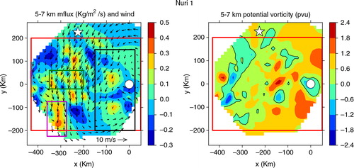
Significant rotation existed at all levels in Nuri 1, with the approximate, system-relative circulation centre at 5–7 km, indicated in Fig. 1 by a white dot. This is located at ) at a reference time of 25.8 hr after 00 UTC on 15 August, and is midway between two mesoscale circulations. The x–y coordinate system is centred on the 5–7 km circulation. The centre of the low-level circulation, indicated by a white star, is located about 300 km to the northwest of the 5–7 km circulation centre, as indicated in Raymond and López Carillo (2011).

The right panel of Fig. 1 shows that the potential vorticity has significant fine-grain structure, but is concentrated in the eastern half of the observed region, largely coincident with the stratiform area. The 5–7 km circulation centre is located near the centre of the region of strong potential vorticity in this layer.

The axisymmetry parameter is plotted for Nuri 1 as a function of radius r and height z relative to the 5–7 km circulation centre in the left panel of Fig. 2. As is clear from Fig. 1, fine structure near the centre results in large values of However, except for the surface and elevations above 8 km, the circulation is relatively close to axisymmetry beyond 100–150 km. The flow is most symmetric at elevations near 4 km.

Fig. 2.  Plots of axisymmetry parameter as a function of radius and height for Nuri 1 (left panel) and Nuri 2 (right panel). The radius is defined relative to the 5–7 km centre. Darker shades indicate a closer approach to axisymmetry.

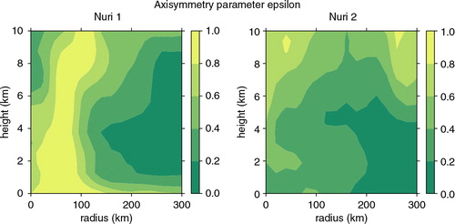
The actual degree of axisymmetry for Nuri 1 is somewhat uncertain because measurements were not made far to the east of the 5–7 km circulation centre. Visual observation from research aircraft showed that this region was clear, probably due to suppression of the boundary layer by the dissipating convection on the east side of Nuri 1.

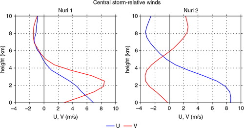
The left panel of Fig. 3 shows the storm-relative wind profile at the approximate centre of the 5–7 km circulation. Substantial shear exists in both components of the wind at this location, with low-level flows generally from the southwest relative to the moving system.

Fig. 3.  Storm-relative zonal (U) and meridional (V) winds as a function of height at the centre of the 5–7 km circulation for Nuri 1 (left panel) and Nuri 2 (right panel).

3.2. Nuri 2

Figure 4 shows a plan view of Nuri 2 at 5–7 km elevation. The vortical circulation at this level is stronger and more organised compared to Nuri 1. Furthermore, a region of intense convective mass flux exists very near the centre of the circulation at this level. We take Raymond et al.'s (2011) system propagation velocity of . The 5–7 km circulation centre (white dot) is located at (140.1°E, 14.7°N) at a reference time of 23.9 hr after 00 UTC on 16 August. The low-level circulation (white star) is located approximately 200 km north of the mid-level circulation.

Fig. 4.  Plan view of Nuri 2 averaged over the elevation range 5–7 km. The left panel shows the vertical mass flux and the system-relative winds. The right panel shows the Ertel potential vorticity, with black contours indicating zero values. The white dot shows the assumed disturbance center in the 5–7 km elevation range while the white star shows the storm-relative circulation center in the 0–2 km range. The red (overall), green (central), and magenta (north) boxes define averaging regions to be discussed later.

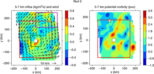
As the right panel of Fig. 4 shows, the potential vorticity for Nuri 2 is more organised and stronger than for Nuri 1, though it still retains significant fine-grain structure. As the right panel of Fig. 2 shows, the circulation is much more axisymmetric close to the circulation centre with the exception of regions above 8 km. The shear at low levels continues to be strong (right panel of Fig. 3), with storm relative flow weakly from the east at the position of the 5–7 km circulation centre.

4. Inversion results

In this section we approximate the potential vorticity distributions in Nuri 1 and Nuri 2 as axially symmetric distributions that take the form of an ambient profile plus Gaussian perturbations:12

The ambient profile is assumed to be13

where f ₀ is the value of the Coriolis parameter centred on the disturbance of interest, is the vertical profile of atmospheric density, and is the z-derivative of potential temperature . The mean vertical gradient of potential temperature over the domain of the TCS030 case is taken to represent ambient tropical conditions in the west Pacific, and is approximated by14

where is the moist adiabatic potential temperature gradient for a surface temperature of 300.5 K and relative humidity of 79%, C=0.96 represents the deviation from a moist adiabat, and the parameters , h _S =3.5 km, and w _S =1.5 km account for the stable layer found near the freezing level in the tropics (Johnson et al., 1996, 1999; Folkins and Martin, 2005). Along with each potential vorticity perturbation component is a surface potential temperature anomaly with the same horizontal structure as the associated potential vorticity anomaly:15

Experience shows that the effect of the surface potential temperature on the potential temperature profile is greatest in the lowest 2 km for the disturbances studied here. Above that level the potential temperature is controlled primarily by the potential vorticity anomaly.

We now describe the individual cases. Table 1 shows the values of parameters used to construct the potential vorticity and surface potential temperature perturbations in (12) for both Nuri 1 and Nuri 2. These values were obtained by an extensive process of trial and error, and as such are not necessarily optimal. However, the values listed produce rough agreement between the balanced model and observations. The surface potential temperature anomaly was set to match observation.

Table 1. Parameters controlling the perturbation potential vorticity and surface potential temperature distributions

Case	i	q i	r i	h i	w i	q Si
Nuri 1	1	1.2 pvu	175 km	5.0 km	4.0 km	−3.5 K
	2	0.1	400	2.0	1.5	0
	3	–1.5	50	6.0	4.5	0
Nuri 2	1	1.3	250	6.0	3.0	–3.0
	2	0.3	400	1.5	2.0	0

4.1. Nuri 1

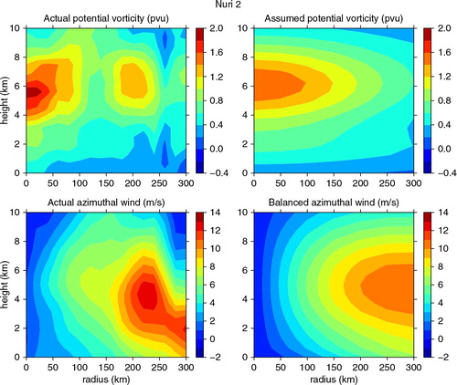
Figure 5 shows the azimuthally averaged azimuthal wind and potential vorticity for Nuri 1. The assumed pattern for the potential vorticity is in rough agreement in scale and magnitude with the observations, though given its simplicity, it cannot reproduce the details of the observed pattern. The azimuthal wind pattern derived from the potential vorticity inversion is in approximate agreement with observations, though the wind maximum is slightly weaker, higher, and closer to the centre than observed.

Fig. 5.  Comparison of azimuthally averaged potential vorticity (upper panels) and azimuthal wind (lower panels) for observations (left panels) and idealised balance model (right panels). The white region in the upper left panel indicates values of potential vorticity less than −0.4 pvu.

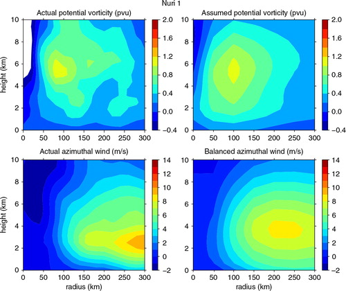
The upper panel of Fig. 6 shows the potential vorticity profile for Nuri 1 averaged over the domain bounded by the red box in Fig. 1. This box encompasses both the convective and stratiform regions of Nuri 1. The thick red line shows the ambient potential vorticity profile, as defined by eq. (13). The near-coincidence of the balanced model and observed potential vorticity profiles indicates that our trial-and-error fitting procedure works well.

Fig. 6.  Horizontally averaged potential vorticity (upper panel) and virtual potential temperature perturbation (lower panel) for Nuri 1. The thick dashed red line in the upper panel represents the ambient potential vorticity, while the thinner dashed red lines represent areally averaged observations in both panels. The solid blue lines show the averages over a corresponding region in the balanced model result.

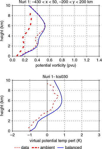
The lower panel of Fig. 6 shows the average observed and balance model virtual potential temperature profiles in Nuri 1. The balance model profile is about 0.3 K warmer than the observed profile; other than this offset, the agreement between the two is remarkably good, indicating that, at least on the average, the virtual temperature structure is close to a balanced state.

Figure 7 shows the meridionally averaged balance model and observed virtual potential temperature patterns as a function of x and z. Though differing in detail, these two patterns are broadly similar.

Fig. 7.  East–west section of Nuri 1 meridionally averaged over −200 km ≤ y ≤200 km. The upper panel shows the balance model prediction for the virtual temperature anomaly as a function of x and z. The middle panel shows the observed virtual temperature anomaly (actual Nuri 1 virtual temperature minus the mean virtual temperature for TCS030) while the bottom panel shows the vertical mass flux. The black vertical bars delimit the convective and stratiform regions. Zero contours are represented by thin black lines.

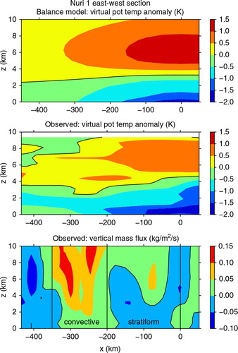
Also shown in Fig. 7 is the vertical mass flux, subject to the same meridional averaging. As noted previously, convection appeared to form at the western edge of Nuri 1, move eastward relative to the system as it evolved, and dissipate on the eastern edge. This evolution is evident in Fig. 7, with convective vertical mass fluxes in the range −350 km≤ x ≤−200 km and stratiform fluxes marked by ascent in the upper troposphere and descent in the lower troposphere to the east of this region. Descent exists to the west of the convective region (x<−350 km).

Figure 8 shows an averaged north–south section of the vertical mass flux in Nuri 1 in the same vein as the bottom panel of Fig. 7. The strongest zonally averaged convection occurs in the range −20 km ≤ y ≤ 60 km with stratiform-like profiles to the south and mainly sinking motion to the north.

Fig. 8.  North-south section of Nuri 1 zonally averaged over −430 km ≤ x ≤50 km showing the vertical mass flux. The black vertical bars delimit the convective and stratiform regions. Zero contours are represented by thin black lines.

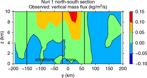
Comparing Figs. 7 and 8 suggests that the strongest vertical mass fluxes occur within the bounds of the green box in Fig. 1. We refer to this as the north convective region. The magenta box to the south, referred to as the south convective region, contains significant convection as well, but this shows up less strongly in the zonal average than the north convective region. Little deep convective mass flux shows up in the vicinity of the low-level circulation, indicated by the star in Fig. 1. The black box in Fig. 1 encompasses most of the stratiform region of Nuri 1.

Figure 9 shows profiles of virtual potential temperature anomalies averaged over the north and south convective regions and the stratiform region in the left panel for Nuri 1. These profiles take a dipolar form with warm anomalies in the upper troposphere and cool anomalies below. Measured profiles averaged over the respective regions are noisy, as is to be expected in the vicinity of strong convection. For this reason the balanced profiles are emphasised as thick, solid lines. As the stratiform region is collocated with the strongest potential vorticity anomaly, the virtual potential temperature anomaly is the strongest there.

Fig. 9.  Profiles of balanced virtual potential temperature perturbation (thick lines) and observed values (thin dashed lines) (left panel), observed relative humidity (middle panel), and observed vertical mass flux (right panel) for averages over the north convective region (green), south convective region (magenta), and the stratiform region (black), as defined in the left panel of Fig. 1.

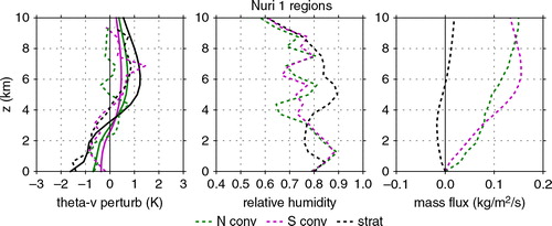
The middle panel of Fig. 9 shows average profiles of relative humidity in the three regions. The stratiform region is drier than the others up to 3 km and more moist above this level.

Vertical mass flux profiles averaged over the three regions defined above are shown in the right panel of Fig. 9. The profiles in the two convective regions are similar, with slightly stronger vertical mass flux at low levels in the north convective region. However, the south convective region's mass flux profile peaks near 6 km, while the maximum for the north convective region is somewhat higher at 10 km. The stratiform region shows a weak stratiform profile with descent in the lower troposphere and ascent in the upper troposphere.

4.2. Nuri 2

Figure 10 shows the azimuthally averaged azimuthal wind and potential vorticity for Nuri 2. As in the case of Nuri 1, the agreement between observation and the balanced model is approximate. The fine-grain structure of the potential vorticity is clearly not captured and the strong azimuthal wind near 300 km range and 1 km elevation is not represented. Perhaps this corresponds to a larger-scale flow arising from potential vorticity anomalies outside the observed region.

Fig. 10.  Comparison of azimuthally averaged potential vorticity (upper panels) and azimuthal wind (lower panels) for observations (left panels) and idealized balance model (right panels).

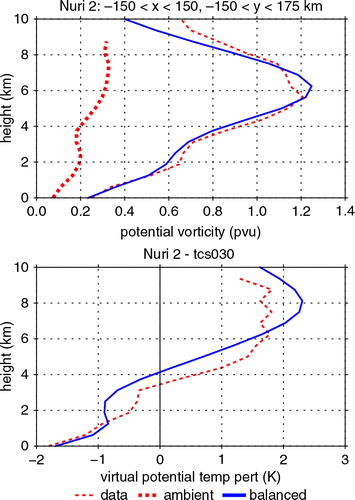
In spite of the crudeness of the axially symmetric representation of the real flow, the observed mean virtual temperature profile is represented reasonably well by the balanced calculation, as Fig. 11 shows. In contrast to Nuri 1, the balanced virtual potential temperature profile is slightly cooler than the actual profile for Nuri 2.

Fig. 11.  Horizontally averaged potential vorticity (upper panel) and virtual potential temperature perturbation (lower panel) for Nuri 2. The thick dashed red line in the upper panel represents the ambient potential vorticity, while the thinner dashed red lines represent areally averaged observations in both panels. The solid blue lines show the averages over a corresponding region in the balanced model result.

Figures 12 and 13 show east–west and north–south cross-sections for Nuri 2. Unlike Nuri 1, strong convection exists at the centre of the 5–7 km circulation. This convection has a very bottom-heavy mass flux profile, as Figs. 12 and 13 show. Stratiform-like mass flux profiles are less evident than in Nuri 1.

Fig. 12.  East-west section of Nuri 2 meridionally averaged over −150 km ≤ y ≤150 km. The upper panel shows the balance model prediction for the virtual temperature anomaly as a function of x and z. The middle panel shows the observed virtual temperature anomaly (actual Nuri 1 virtual temperature minus the mean virtual temperature for TCS030) while the bottom panel shows the vertical mass flux. The black vertical bars delimit the convective region. Zero contours are represented by thin black lines.

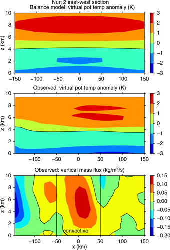
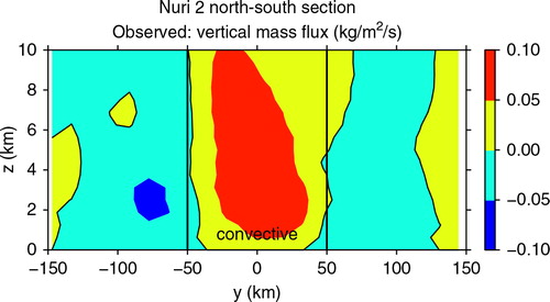
Fig. 13.  North-south section of Nuri 2 zonally averaged over −150 km ≤ x ≤150 km showing the vertical mass flux. The black vertical bars delimit the convective and stratiform regions. Zero contours are represented by thin black lines.

The left panel of Fig. 14 shows the virtual temperature perturbation profiles for two convecting regions in Nuri 2, the central region collocated with the 5–7 km circulation centre and a region well north of the centre. The observed profiles exhibit a dipole structure as in Nuri 1. The balanced profiles in the two regions are in reasonable agreement with the observed profiles. The dipole in virtual potential temperature is stronger by nearly a factor of 2 for both regions studied in comparison to the Nuri 1 case, and is significantly stronger for the central region than for the northern region in both data and in the balanced calculation.

Fig. 14.  Profiles of balanced virtual potential temperature perturbation (thick lines) and observed values (thin dashed lines) (left panel), observed relative humidity (middle panel), and observed vertical mass flux (right panel) for averages over the central (green) and north (magenta) regions of Nuri 2, as defined in the left panel of Fig. 4.

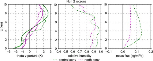
The relative humidity profiles for Nuri 2, shown in the centre panel of Fig. 14, are moister at middle levels than for Nuri 1. Within the Nuri 2 case, the centre is more moist than the north.

The mass flux profiles shown in the right panel of Fig. 14 are both more bottom-heavy than in Nuri 1. However, the mass flux in the central region of Nuri 2 is significantly more bottom-heavy than that in the northern region, with a maximum vertical mass flux near an elevation of 3 km. (Maximum magnitudes of mass flux profiles should not be compared, as averaging in different cases includes different non-convective areal fractions.)

4.3. Summary

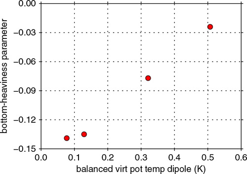
Examination of Fig. 9 and 14 suggests that the stronger the virtual potential temperature dipole in a given region, the more bottom-heavy is the vertical mass flux profile. Figure 15 quantifies this for the small number of cases available by plotting a measure of the bottom-heaviness,16

Fig. 15.  Bottom-heaviness parameter B vs. the strength of the balanced virtual potential temperature dipole D for the profiles presented in Figs. 9 and 14.

vs. the strength of the balanced virtual potential temperature dipole,17

In these equations h=10 km is the depth of the region studied, M(z) is the vertical mass flux profile, and is the balanced virtual potential temperature perturbation produced by the potential vorticity inversion. The quantity B becomes larger as the mass flux profile becomes more bottom-heavy. The stratiform region of Nuri 1 is not included, as no significant convection was occurring in this region.

Though the number of cases is small, Fig. 15 strongly suggests that balanced warming aloft and cooling at lower levels results in more bottom-heavy convection.

5. Discussion and conclusions

In this study, we have approximated the observed potential vorticity distributions in two cases, the first and second missions into the developing typhoon Nuri in 2008, by axisymmetric distributions of potential vorticity. These potential vorticity distributions were then inverted under the non-linear balance condition to obtain balanced flow patterns and virtual potential temperature distributions. Observed low-level potential temperature values were used to define the lower boundary conditions for the inversion. Virtual potential temperature perturbations were defined relative to the observed mean virtual potential temperature profile for the TCS030 case, which was a weak, non-developing tropical wave (see Raymond and López Carillo, 2011; Raymond et al., 2011).

The mean balanced virtual potential temperature profiles obtained in the above inversions were approximately the same as the observed profiles in the two Nuri cases, indicating that overall, the flows were roughly in non-linear balance.

Comparison of observed and balanced potential temperature profiles for specific regions within the developing cyclone was less good in both cases. However, stronger balanced virtual potential temperature dipoles in the defined regions were correlated with more bottom-heavy convection. This supports the weak temperature gradient cloud-resolving model results of Raymond and Sessions (2007).

The exception to the above rule was the eastern region of the first Nuri case. The boundary layer in this region was depleted to the extent that no convection was being initiated; the mass flux there showed a weak stratiform pattern. Given the observed eastward propagation of convection through Nuri on this day, one would expect the deep convection further to the west to become stratiform, thus extending the eastern stratiform region to the west in phase with the motion of the tropical wave.

The normal fate of depleted boundary layers in stratiform regions is regeneration by surface fluxes over a 6–12 hr period (Zipser, 1969), followed by the resurgence of deep convection. Given the strong, balanced virtual temperature dipole present in the stratiform region in this case, one would expect the new convection in this region to exhibit a bottom-heavy mass flux profile, resulting in the spin up of a low-level circulation. We hypothesise that the intense convection observed on the following day near the centre of the mid-level circulation resulted from this mechanism.

The main contribution of the present work is the demonstration that the virtual potential temperature dipole that occurs in a developing tropical cyclone is not a transient result of the convection itself, but is a balanced response to a large region of mid-level vorticity. This supports the mechanism for tropical cyclogenesis proposed by Raymond et al. (2011).

This study represents a first attempt to determine the balanced flow and virtual potential temperature patterns associated with the potential vorticity patterns observed in developing tropical storms. The results are encouraging enough to justify the exploration of inversions of actual potential vorticity distributions in a broad variety of cases.

Acknowledgements

Thanks to Saška Gjorgjievska, Stipo Sentić, Sharon Sessions, Kerry Emanuel and an anonymous reviewer for helpful comments on this study. This work was supported by US National Science Foundation Grants 1021049 and 0851663 and Office of Naval Research Grant N000140810241.

References

- Bister M. Emanuel K. A. The genesis of hurricane Guillermo: TEXMEX analyses and a modeling study. Mon. Wea. Rev. 1997; 125: 2662–2682.
- Bolin B. Numerical forecasting with the barotropic model. Tellus. 1955; 7: 27–49. 10.3402/tellusa.v64i0.19181.
- Bolin B. An improved barotropic model and some aspects of using the balance equations for three-dimensional flow. Tellus. 1956; 8: 61–75. 10.3402/tellusa.v64i0.19181.
- Charney J. G. The use of primitive equations of motion in numerical prediction. Tellus. 1955; 7: 22–26. 10.3402/tellusa.v64i0.19181.
- Cho H.-R. Jenkins M. A. The thermal structure of tropical easterly waves. 1987; 44: 2531–2539.
- Davis C. A. Piecewise potential vorticity inversion. J. Atmos. Sci. 1992; 49: 1397–1411.
- Davis C. A. Trier S. B. Mesoscale convective vortices observed during BAMEX. Part I: Kinematic and thermodynamic structure. J. Atmos. Sci. 2007; 135: 2029–2049. 10.3402/tellusa.v64i0.19181.
- Elsberry R. L. Harr P. A. Tropical cyclone structure (TCS08) field experiment science basis, observational platforms, and strategy. Mon. Wea. Rev. 2008; 44: 209–231.
- Folkins I. Martin R. V. The vertical structure of tropical convection and its impact on the budgets of water vapor and ozone. Asia-Pacific J Atmos Sci. 2005; 62: 1560–1573. 10.3402/tellusa.v64i0.19181.
- Hoskins B. J. McIntyre M. E. Robertson A. W. On the use and significance of isentropic potential vorticity maps. J. Atmos. Sci. 1985; 111: 877–946. 10.3402/tellusa.v64i0.19181.
- Johnson R. H. Ciesielski P. E. Hart K. A. Tropical inversions near the 0°C level. Quart. J. Roy. Meteor. Soc. 1996; 53: 1838–1855.
- Johnson R. H. Rickenbach T. M. Rutledge S. A. Ciesielski P. E. Schubert W. H. Trimodal characteristics of tropical convection. J. Atmos. Sci. 1999; 12: 2397–2418.
- Lorenz E. N. Energy and numerical weather prediction. J. Climate. 1960; 12: 364–373. 10.3402/tellusa.v64i0.19181.
- McWilliams J. C. A uniformly valid model spanning the regimes of geostrophic and isotropic, stratified turbulence: Balanced turbulence. Tellus. 1985; 42: 1773–1774.
- Montgomery, M. T, Lussier III, L. L, Moore, R. W and Wang, Z, 2010. The genesis of Typhoon Nuri as observed during the Tropical Cyclone Structure 2008 (TCS-08) field experiment – Part 1: The role of the easterly wave critical layer. J. Atmos. Sci. 10, 9879–9900. 10.3402/tellusa.v64i0.19181.
- Montgomery M. T. Smith R. K. The genesis of Typhoon Nuri as observed during the Tropical Cyclone Structure 2008 (TCS08) field experiment – Part 2: Observations of the convective environment. Atmos. Chem. Phys. 2012; 12: 4001–4009. 10.3402/tellusa.v64i0.19181.
- Peixoto, J. P and Oort, A. H. 1992. American Institute of Physics, College Park, Maryland, pp. 520.
- Raymond D. J. Nonlinear balance and potential-vorticity thinking at large Rossby number. Physics of climate. 1992; 118: 987–1015. 10.3402/tellusa.v64i0.19181.
- Raymond D. J. Nonlinear balance on an equatorial beta plane. Quart. J. Roy. Meteor. Soc. 1994; 120: 215–219. 10.3402/tellusa.v64i0.19181.
- Raymond D. J. Testing a cumulus parametrization with a cumulus ensemble model in weak-temperature-gradient mode. Quart. J. Roy. Meteor. Soc. 2007; 133: 1073–1085. 10.3402/tellusa.v64i0.19181.
- Raymond D. J. López Carrillo C. The vorticity budget of developing typhoon Nuri (2008). Quart. J. Roy. Meteor. Soc. 2011; 11: 147–163. 10.3402/tellusa.v64i0.19181.
- Raymond, D. J and Sessions, S. L. 2007. Evolution of convection during tropical cyclogenesis. Atmos. Chem. Phys. 34, L06811. DOI:10.3402/tellusa.v64i0.19181.
- Raymond, D. J, Sessions, S. L and López Carrillo, C. 2011. Thermodynamics of tropical cyclogenesis in the northwest Pacific. Geophys. Res. Letters. 116, D18101. DOI: 10.3402/tellusa.v64i0.19181.
- Raymond D. J. Zeng X. Modelling tropical atmospheric convection in the context of the weak temperature gradient approximation. J. Geophys. Res. 2005; 131: 1301–1320. 10.3402/tellusa.v64i0.19181.
- Reed R. J. Recker E. E. Structure and properties of synoptic-scale wave disturbances in the equatorial western Pacific. Quart. J. Roy. Meteor. Soc. 1971; 28: 1117–1133.
- Schubert W. H. Alworth B. T. Evolution of potential vorticity in tropical cyclones. J. Atmos. Sci. 1987; 113: 147–162. 10.3402/tellusa.v64i0.19181.
- Sobel A. H. Bretherton C. S. Modeling tropical precipitation in a single column. Quart. J. Roy. Meteor. Soc. 2000; 13: 4378–4392.
- Sobel A. H. Nilsson J. Polvani L. M. The weak temperature gradient approximation and balanced tropical moisture waves. J. Climate. 2001; 58: 3650–3665.
- Thorpe A. J. Diagnosis of balanced vortex structure using potential vorticity. J. Atmos. Sci. 1985; 42: 397–406.
- Zipser E. J. The role of organized unsaturated convective downdrafts in the structure and rapid decay of an equatorial disturbance. J. Atmos. Sci. 1969; 8: 799–814.