The EUMETSAT OSI SAF near 50 GHz sea ice emissivity model

ABSTRACT

A sea ice thermal microwave emission model for 50 GHz was developed under EUMETSAT's Ocean and Sea Ice Satellite Application Facility (OSI SAF) programme. The model is based on correlations between the surface brightness temperature at 18, 36 and 50 GHz. The model coefficients are estimated using simulated data from a combined thermodynamic and emission model. The intention with the model is to provide a first guess sea ice surface emissivity estimate for atmospheric temperature sounding applications in the troposphere in numerical weather prediction (NWP) models assimilating Advanced Microwave Sounding Unit (AMSU) and Special Sensor Microwave Imager/Sounder (SSMIS) data. The spectral gradient ratio is defined as the difference over the sum of the SSMIS brightness temperatures at 18 and 36 GHz vertical linear polarisation (GR1836). The GR1836 is related to the emissivity at the atmospheric temperature sounding channels at around 50 GHz. Furthermore, the brightness temperatures and the polarisation ratio (PR) at the neighbouring 18, 36 and 50 GHz channels are highly correlated. Both the gradient ratio at 18 and 36 GHz and the PR at 36 GHz measured by SSMIS are input into the model predicting the 50 GHz emissivity for horizontal and vertical linear polarisations and incidence angles between 0° and 60° The simulated emissivity is compared to the emissivity derived with alternative methods. The fit to real AMSU observations is investigated using the different emissivity estimates for simulating the observations with atmospheric data from a regional weather prediction model.

• sea ice
• microwave emissivity modelling
• atmospheric temperature sounding

1. The OSI SAF sea ice emissivity model

The microwave sea ice surface emissivity is relevant when applying the radiative transfer equation for simulating the top of the atmosphere up-welling Earth emission measured by satellite radiometers. Here, we present a model for estimating the sea ice microwave near 50 GHz emissivity.

The ocean and sea ice satellite application facility (OSI SAF) near 50 GHz sea ice emissivity model is based on correlations between the surface brightness temperature at 18, 36 and 50 GHz. The model coefficients are tuned with simulated data from a combined thermodynamic and emission model (Tonboe, 2005, 2010; Tonboe et al., 2011). The intention with the model is to provide a first guess sea ice surface emissivity estimate for atmospheric temperature sounding applications in the troposphere in numerical weather prediction (NWP) models assimilating Advanced Microwave Sounding Unit (AMSU) and Special Sensor Microwave Imager/Sounder (SSMIS) data. The spectral gradient ratio defined as the difference over the sum of the 18 and 36 GHz window channels at vertical polarisation (GR1836) is related to the emissivity at the atmospheric temperature sounding channels at around 50 GHz (Tonboe, 2010). Further, the brightness temperatures and the polarisation ratio (PR) at neighbouring channels are highly correlated, that is, the PR at 36 GHz (PR36) and the PR at 50 GHz (PR50). Both the gradient ratio and the PR measured by conically scanning radiometers SSM/I and SSMIS currently in orbit are inputted to the model predicting the near 50 GHz emissivity for horizontal and vertical linear polarisations and incidence angles between 0° and 60°. This model can attain solutions in between perfectly diffuse emission and the specular reflection determined by Fresnel reflection coefficients. In addition, the OSI SAF project is providing daily grids of the model coefficients, the nadir emissivity for AMSU and the emissivity at vertical polarisation at 50° for SSMIS. The emissivity estimate is given for both sea ice and ice shelves in the Arctic and around Antarctica.

Several operational weather centres have tested the assimilation of surface sensitive microwave sounding channels over land and sea ice (Heygster et al., 2009; Karbou et al., 2010). Different approaches have been applied for treating the surface emission part of the signal. For example, test runs described in Heygster et al. (2009) with the regional numerical weather prediction model High Resolution Local Area Model (HIRLAM) where satellite microwave radiometer data from sea ice covered regions were assimilated indicated that atmospheric temperature sounding over sea ice is feasible. The test runs used a simple sea ice surface emissivity model where the emissivity estimate is a function of GR1836. The test showed that the assimilation of AMSU near 50 GHz temperature sounding data over sea ice improved model skill on common variables such as surface temperature, wind and air pressure (Heygster et al., 2009). These applications, where the surface emission is needed for estimating temperature in the lower troposphere, are the motivation for the new OSI SAF sea ice emissivity model. Satellite sounding over sea ice is of particular interest because of the scarcity of conventional sounding data, that is, aircraft ascents and radiosonde data. Variational data assimilation schemes for NWP models may use surface emissivity derived from near real time emissivity maps either directly into the observation operator or as a first guess. However, this is only possible when there is a reasonably good fit between simulations and observations. In this study, we analyse the fit between the simulations and the AMSU-A sounding observations using the simulated surface emissivity from the OSI SAF model. Further, the OSI SAF model is compared to other methods that have been used earlier for deriving sea ice emissivity. The analysis period covers the autumn freeze-up from 19 October to 30 November 2011, and it uses atmospheric data from the operational HIRLAM model. If there is a good fit between simulations and observations using the OSI SAF model surface emissivity, then it is possible to use the simulated surface emissivity for assimilation trials and thereby assess its impact for a specific NWP model.

1.1. Sea ice emissivity compared to other surface types

For sea ice there is a large vertical and lateral surface heterogeneity within the footprint including significant microwave penetration into the snow and ice and across the temperature gradient beneath the surface meaning that the surface temperature is not synonymous with the effective temperature (Mathew et al., 2008). The effective temperature is the integrated emitting layer thermometric temperature. The sea ice effective temperature is also important for the atmospheric sounding applications (English, 2008). The effective temperature is described in Tonboe et al. (2011) and in section 5. Over land, emissivity climatology is used as a first-guess in atmospheric sounding applications (Aires et al., 2010). However, sea ice is dynamic: it drifts, deforms, melts or forms from day to day which means that the current emissivity cannot be derived from emissivity climatology.

For smooth soil surfaces, the surface reflectivity is specular, otherwise for rough surfaces the specular model can be adjusted using a single-parameter (roughness) model (Ulaby et al. 1982, p. 889), that is,1

where r is the reflectivity at incidence angle θ and vertical (v) or horizontal (h) linear polarisation p. The subscript sp is for specular, that is, the Fresnel reflection coefficient and h′ is a roughness parameter.

Several models link the physical snow and ice properties with the microwave emission (e.g. Weng et al., 2001; Mätzler et al., 2006). Mixtures between different surface scattering models are common in land surface emission models. For example, the community microwave emission model for land surfaces uses a combination of rough and specular surface scattering where the surface roughness state is derived from auxiliary parameters, that is, land use maps (Drusch et al., 2009) and Mätzler (2005) simulates the emissivity of snow surfaces as a mix between Lambertian and specular scattering.

The sea ice emissivity, at a certain polarisation, frequency and angle with respect to the surface, is a function of surface scattering, subsurface extinction and reflections between layers with different permittivity. Physical models relate the emissivity with the snow and ice properties such as density, temperature, snow crystal and brine inclusion size to microwave attenuation, scattering and reflectivity (Weng et al., 2001; Mätzler et al., 2006). The microwave penetration depth in snow is in the order of centimetres to decimetres due to significant extinction in the snow and in saline ice (Tonboe, 2010). However, the surface emissivity model parameters are not prognostic variables in NWP models. The input parameters are difficult to measure in the field and are a stretch target for detailed process models at present.

Therefore, the microwave emissivity at near 50 GHz is characterised here using a model where the emissivity is a function of the spectral gradient (GR1836) and the PR (PR36) measured at the neighbouring atmospheric window channels at 18 and 36 GHz. The GR1836 and PR36 can be measured with SSM/I and SSMIS sensors currently in orbit. Output from the combined thermodynamic and microwave emission models described in section 2.5 are used for generating the relationships between the 18 and 36 GHz simulated brightness temperatures and the 50 GHz emissivity. The simulated data are described in Tonboe (2010). Both the community model (Drusch et al., 2009) and Mätzler (2005) finds solutions in between two extreme cases. Similarly, the OSI SAF model can attain solutions in between: (1) perfectly diffuse emission where there is no angular dependence and no polarisation difference similar to the model used in Heygster et al. (2009) for AMSU-A; and (2) the specular reflection with the angular dependence and the polarisation determined by the Fresnel reflection coefficients and a surface permittivity of 3.5 which is typical for sea ice. The model is expected to be valid for incidence angles between 0° and 60°.

2. Satellite instruments and data

The model is applicable to two types of sounders currently in orbit, namely the SSMIS and the AMSU. Transmission of microwave radiation through the atmosphere in the range from 18 to 90 GHz is affected primarily by three processes: 1) oxygen absorption particularly from 50 to 70 GHz, 2) water vapour absorption near 22 GHz and 3) scattering from water and ice particles at higher frequencies in particular. At the 50–70 GHz oxygen absorption lines, the atmosphere is virtually opaque and the satellite channels measuring at these frequencies are called sounding channels. However, there is a contribution from the surface at the lower temperature sounding frequencies between 50.3 and 54.4 GHz where microwave penetration is into the troposphere. These frequencies correspond, for example, to channels 3–6 on the AMSU instrument and the channels 1–4 on the SSMIS. The dry polar atmosphere is generally transparent for microwave radiation in between the sounding channels called the atmospheric windows for frequencies less than 22 GHz, between 22 and 50 GHz and from 70 to 118 GHz.

2.1 The microwave sounding unit: AMSU

The AMSU is a whisk broom polar orbiting microwave radiometer with variable incidence angle, footprint size and the linear polarisations are mixed. The AMSU has scan angles between nadir and about ±49° and a swath width of about 2000 km (Mo, 1996). The AMSU data are used in the HIRLAM tests described in section 5.

Provided that the 3rd and 4th Stokes parameters are near 0 over sea ice, the h and v polarisations are mixed as a function of scan angle, θ, on AMSU (Mathew et al., 2008):2

where3

R _e is the Earths radius (6371 km) and H is the height of the satellite above the surface (about 800 km). The 3rd and 4th Stokes parameters are most often near zero during the cold season (Narvekar et al., 2011).

2.2 The special scanning microwave imager sounder: SSMIS

The SSMIS is a polar orbiting conically scanning radiometer with constant incidence angle around 50° and a swath width of about 1700 km. It has window channels near 19, 37, 91 and 150 GHz and sounding channels near 22, 50, 60 and 183 GHz. The SSMIS temperature sounding channels 1–4 near 50 GHz vertical polarisation penetrate into the lower troposphere and partially to the surface (Kunkee et al., 2008).

The OSI SAF emissivity model input data is an internal conversion of the SSMIS SDR BUFR format to NetCDF. The BUFR format files are described in Patterson (2010). The brightness temperatures are from the ‘environmental’ channels on SSMIS, that is, channel 12 (T _h19 ), 13 (T _v19 ), 14 (T _v22 ), 15 (T _h37 ) and 16 (T _v37 ). We use channel 13, 15 and 16. The Tb measured at each of these frequencies has different spatial resolution on the Earth's surface. The resolution (integrated field of view) of the 19 GHz channels is an ellipse about 45×68 km and the 37 GHz channels have a resolution about 3.5 times higher, that is, 24×36 km. The 19 and 37 GHz channels are combined in the emissivity model and in order to reduce noise near emissivity gradients, the 37 GHz channels are re-sampled to the coarser 19 GHz resolution. The resampling is done using a uniform Gaussian weighting function with a standard deviation of 36 km.

2.3. The gradient ratio at 18 and 36 GHz

Brightness temperatures are measured at window frequencies where the sensitivity to the atmosphere is minimised, for example, at 18 and 36 GHz. The spectral gradient (GR1836) is given by the following equation:4

The normalisation reduces the GR1836 sensitivity to thermometric temperature of the target, and ice concentration algorithms use it to correct for first- and multiyear ice types with different scattering magnitudes (Comiso et al., 1997). Though the sensitivity to temperature (T _eff ) is reduced in GR1836, there is still a small dependence due to different microwave penetration at 18 and 36 GHz across the temperature gradient in snow and ice.

2.4 The polarisation ratio at 36 GHz

The PR at 36 GHz, PR36, is given by the difference over the sum of the Tv36 and Th36 brightness temperatures at 36 GHz, that is,5

Also, for the PR the temperature dependence is minimised by the normalisation.

2.5 The model coefficients using simulated data

Simulated data from a combined thermodynamic and emission model is used to derive the coefficients for the OSI SAF 50 GHz emissivity model. These are described in Tonboe (2010) and Tonboe et al. (2011). The data are generated by forcing a thermodynamic model with meteorological data input (Tonboe, 2005). The sea ice emission model relates physical snow and ice properties such as density, temperature, snow crystal and brine inclusion size from the thermodynamic model in a 1-D vertical profile every 6 hours during the winter season to microwave attenuation, scattering, reflectivity, emissivity, effective temperature and brightness temperature. The emission model used here is a sea ice version of MEMLS (Wiesmann and Mätzler, 1999) described in Mätzler et al. (2006). There are six profiles in the Arctic and two profiles in the Antarctic (one in the Ross Sea and one in the Weddell Sea). All simulations are at 50° incidence angle similar to SSMIS and other space-borne conically scanning radiometers. The sea ice emissivity simulations were initially done for the Advanced Microwave Scanning Radiometer (AMSR), and were measured near 18 and 36 GHz instead of at 19 and 37 GHz. This shift in frequency is negligible for the surface emissivity while it is important for the atmospheric emission.

3. The model coefficients

The sea ice emissivity at 50 GHz is related to the GR1836. Simulated data for both the vertical and horizontal polarisation at an incidence angle of 50° are shown in Fig. 1. The GR1836 Arctic tie-points for first and multiyear ice are shown in Fig. 1. The tie-points from Comiso et al. (1997) represent typical values for the two ice types, respectively.

Fig. 1.  The simulated multiyear ice GR1836 versus the e50v (black) and e50h (grey). The best fit line to the e50v is: e50v=3.16GR1836+0.97 and for e50h: e50h=2.48GR1836+0.90. The dashed lines show the ±2%. The vertical grey lines indicate the tie-points for first- (F) and multiyear (M) ice, respectively.

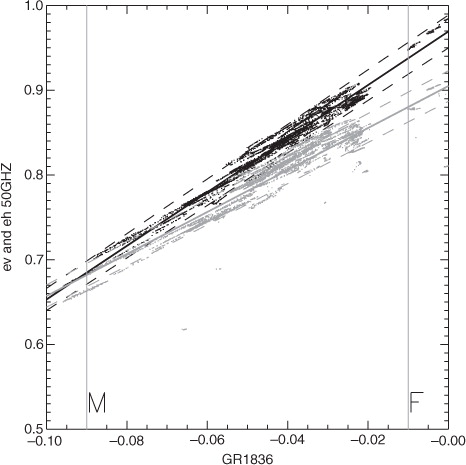
Lines have been fitted to the data clusters representing simple models for the emissivity at 50° incidence angle, that is,6

and7

It is noted that both the emissivity and polarisation difference are decreasing as a function of larger negative GR1836. Most of the simulated data points are within ±2% of the fitted lines and the model-data RMS for vertical polarisation is 0.008 (for the southern hemisphere the RMS is 0.01) and the RMS is 0.019 for horizontal polarisation. The crossover of the fitted lines in Fig. 1 shows the limitations of this linear model outside of the natural range of emissivities and for deriving the polarisation difference. The v–h polarisation difference is always positive.

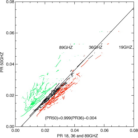
The relationship between PR36 and PR50 is shown in Fig. 2 together with 18 and 89 GHz PRs. The PR is decreasing from 18 to 36 to 50 to 89 GHz. In the model, the PR at 36 GHz is used as a proxy for the polarisation difference at 50 GHz. The model and data difference RMS for the 36 GHz PR and the 50 GHz PR is 0.0014. The same processes determine the polarisation difference at 36 and 50 GHz.

Fig. 2.  The simulated sea ice PR18 in red, PR36 in black and PR89 in green versus the PR50. The fitted line to the PR36 versus PR50 cluster is PR50=0.999PR36-0.004.

Using the linear relationships in Figs. 1 and 2 based on the simulated data, it is now possible to estimate the 50 GHz emissivity at 50° incidence at vertical and horizontal polarisations in terms of GR1836 and PR36.

We propose a simple model for extrapolating the GR1836 emissivity proxy and the PR36 polarisation proxy for SSMIS to the range of incidence angles (θ) and h and v polarisations on AMSU using the reflection coefficients for sea ice. The specular reflection coefficients for vertical, r _v and horizontal, r _h , polarisations are given in terms of the sea ice permittivity ɛ (ɛ=3.5) and θ the angle of incidence, that is,8 9

3.5 is a typical value for the sea ice permittivity (Ulaby et al., 1986). The permittivity is normally expressed as a complex number where the imaginary component is called the loss factor. It is common to neglect the sea ice loss factor when computing the reflection coefficients. However, even if the loss is considered, for example, the permittivity is 3.5+0.5j instead of 3.5, which is a high loss factor typical for relatively warm and saline sea ice, then the difference in emissivity between permittivities 3.5 and 3.5+0.5j is less than 0.003 between 0° and 60°. For 3.5 and 3.5+0.1j, which is realistic for cold ice, it is less than 0.0002. These differences are small compared to other uncertainties.

The 50 GHz emissivity is in terms of the two parameters S and R:10

and11

The RMS between the emissivity from the radiative transfer model (in Tonboe et al., 2011) and the model in eq. (10) and (11) at 50° incidence angle is 0.0093 for vertical polarisation and 0.0071 for horizontal polarisation. In the Ulaby et al. (1982) model shown in eq. (1), R is a surface roughness parameter because the relationship between the PR36 and PR50 R is given as a function of PR36 here. For R=0, the scattering at the surface is totally diffuse and for R=1 the scattering is specular. R=1 for PR36=0.11 for a sea ice permittivity of 3.5. A third-degree polynomial is fitted to the simulated data (Tonboe, 2010) using least squares for the northern and southern hemisphere, that is,12a 12b

and S as a function of GR1836 using least squares and a linear fit:13a 13b

4. The OSI SAF emissivity model results

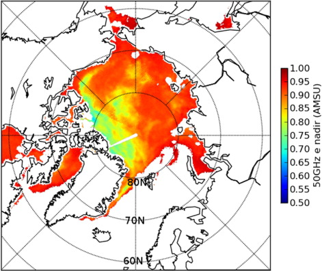
The 50 GHz nadir emissivity of first year ice in the Arctic is from 0.9 to near 1 as seen in Fig. 3. The Arctic multiyear ice emissivity is from 0.7 to 0.8. Therefore, the geographic variability of the Arctic emissivity is with the highest emissivities over the Siberian shelves, the Baffin Bay and Hudson Bay. The lowest emissivities are found north of Greenland.

Fig. 3.  The nadir emissivity on 17 January 2012. The latitude is marked along the 0° longitude.

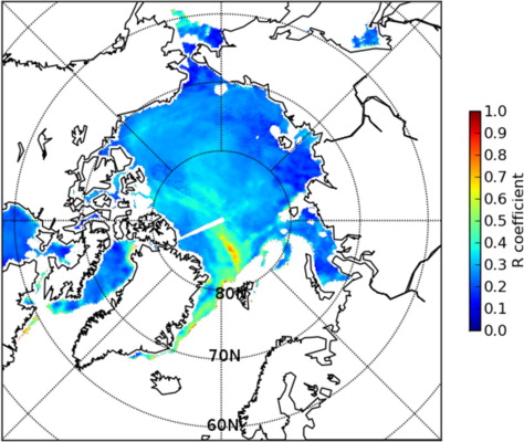
The polarisation parameter, R, shown in Fig. 4 is between 0.2 and 0.4 in the Arctic but locally is near 0.8 in the ice-covered Greenland Sea.

Fig. 4.  The R coefficient on 17 January 2012. The latitude is marked along the 0° longitude.

On the southern hemisphere, the emissivity variability is higher than in the Arctic. The emissivity varies between 0.5 and near 1, as seen in Fig. 5. The emissivity variability on the southern hemisphere is caused by different snow cover conditions (Willmes et al., 2011).

Fig. 5.  The nadir emissivity on 17 January 2012. The latitude is marked along the 180° longitude.

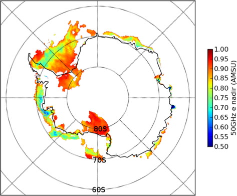
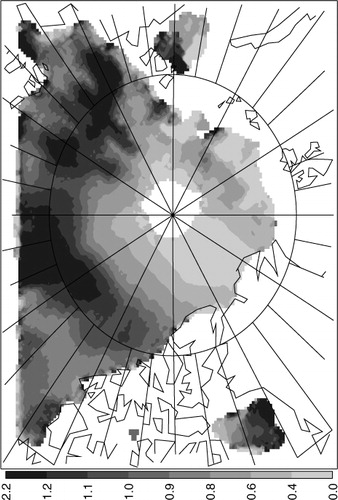
On the southern hemisphere, R is typically between 0.2 and 0.5 while extensive areas in both the Ross and Weddell Sea are near 1 (Fig. 6).

Fig. 6.  The R coefficient on 17 January 2012. The latitude is marked along the 180° longitude.

The variability of the S parameter is similar to the nadir emissivity variability on both the northern and the southern hemisphere. The S parameter is therefore not shown here.

The R parameter indicates the level of specularity. The completely specular situation in this model (for R=1) is a plane ice surface with a permittivity of 3.5. Scattering is diffuse when R=0. Diffuse emission is uniform and independent of incidence angle and polarisation. Physically, diffuse emission is associated with rough surfaces and volume scattering (Harlow, 2011).

5. Evaluation of the OSI SAF sea ice emissivity model fit during freeze-up

The OSI SAF emissivity model is evaluated using the model sea ice surface emissivity estimate with the surface temperatures and the atmospheric profiles from the regional High-Resolution Limited-Area Model (HIRLAM) atmospheric model to simulate the brightness temperature of the AMSU channels peaking in the lower troposphere and being sensitive to the sea ice surface emission. The HIRLAM version applied here is the operational regional NWP model of the Norwegian Meteorological Institute, with 12 km horizontal resolution covering Norway and most of the sea ice covered Arctic Ocean.

The tests were done during the Arctic freeze-up period from 19 October to 30 November 2011. For each AMSU observation point, the OSI SAF emissivity together with HIRLAM surface temperatures and atmospheric temperature profiles have been used as input to the radiative transfer model RTTOV-8 (Saunders et al., 1999) to simulate Tb for comparison with the observed AMSU Tb. This has been repeated with alternative formulations for the sea ice emissivity for comparison. Only satellite footprints where the OSI SAF sea ice concentration is exceeding 95% are included. There is no screening of the data contaminated by clouds which could potentially cause scattering at 50 GHz. Correction for scattering is not included in the model.

Comparison of forward calculations with observations in surface affected channels is seen as a good first approach for assessing the emissivity model, since direct in-situ observations of emissivity on scales of the satellite footprints are unavailable. This use of the sea ice emissivity estimates is comparable to how the emissivity data could be used for data assimilation. However, the forward simulations also need a surface temperature and atmospheric temperature and moisture profiles from the HIRLAM model, that is, the emissivity together with the effective surface temperature is used as input to the RTTOV-8 radiative transfer model simulating the radiation path through the atmosphere. This means that errors related to the atmospheric profiles and the surface temperature affect the comparison.

We see five sources of uncertainty in this comparison causing differences between the output of the forward simulations and the observations: 1) observation uncertainties, 2) the mismatch in time and space between observations and the model representation of them. This is referred to as the representativeness error, 3) the uncertainties in the HIRLAM atmospheric profiles and the surface effective temperature, 4) the uncertainties in the emissivity input to the forward simulation and 5) the forward model uncertainties.

The hypothesis, which we wish to use for the analysis, is that when we only change the simulated surface emissivity estimate and constrain all other variables, a better fit between simulations and observations indicates a more accurate surface emissivity estimate, and the fit is an indication of the quality of the emissivity estimate.

This will generally be the case if the different uncertainties listed above are not correlated. However, if some of the errors corresponding to the uncertainties were anti-correlated with the emissivity error these errors would be compensating each other. It would then not be given that a better fit between simulations and observations would indicate a more accurate surface emissivity estimate as assumed in the hypothesis. We do not expect anti-correlation between errors.

The comparison results presented here are in two parts: 1) comparison of the OSI SAF sea ice emissivity estimate with two different models which we will refer to as the ‘tie-point model’ (Heygster et al., 2009) and the ‘dynamical method’ (Mathew et al., 2008) and 2) comparison of observed AMSU brightness temperatures with corresponding simulated values using RTTOV-8 with HIRLAM atmospheric profiles and the OSI SAF model emissivity.

5.1 Comparison of the sea ice emissivity estimate using different models

Figure 7A shows emissivities computed with the tie-point model versus the OSI SAF model emissivities. There is a high correlation between the emissivities found using the two methods. Both the OSI SAF and the tie-point model are functions of the GR1836. However, the OSI SAF model is not constrained by the tie-points and has a larger dynamic range. In particular the OSI SAF method finds lower multiyear ice emissivities. Adjusting the multiyear ice tie-point in the tie-point model would lower the bias between the methods. Both models have first-year ice emissivities around 0.93. The OSI SAF model gives multiyear ice emissivities around 0.7 while the multiyear ice tie-point in the tie-point method is 0.796. Estimates of Arctic multiyear ice emissivities are given in the literature: Mathew et al. (2008) reports Arctic multiyear ice emissivities in November between 0.6 and 0.8 depending on incidence angle. Kongoli et al. (2011) report typical Arctic multiyear ice emissivities around 0.73. Both of these values from the literature agree more with the estimates from the OSI SAF model than the tie-point model. Also the results of an assimilation study described in Thyness et al. (2005) using the tie-point model indicates that the multiyear ice tie-point is too high.

Fig. 7.  Comparison between predicted emissivities using (A) the tie-point model and the OSI SAF model; (B) the dynamical method and the OSI SAF model. The data are from the AMSU instrument on the NOAA-15 satellite.

The OSI SAF model was also compared to the dynamical method for estimating surface emissivity. The dynamical method emissivity can be derived using a simplified radiative transfer equation and it is described in Mathew et al. (2008) and it has been applied for sounder data assimilation over land (Karbou et al., 2006). It is based on simulations of the brightness temperature using the atmospheric radiative transfer model RTTOV-8 with surface emissivities (e) at zero and at one, that is, Tb _sim (e=0) and Tb _sim (e=1) and AMSU channel 3 (50.3 GHz) brightness temperatures:14

The dynamical method determines the emissivity so that the mismatch between observations and simulated Tbs in the window channel applied for the calculation is minimised.

Figure 7B show the emissivity derived with the dynamical method for AMSU data vs. the OSI SAF model emissivities. There is a high correlation between the two emissivity estimates although the scatter between the two emissivity estimates is large (standard deviation of differences is 0.049 for NOAA-15 (not shown) and 0.047 for NOAA-16). The scatter is larger for higher emissivities (typically first-year ice emissivities). The bias between the two products is small (0.008 for NOAA-16). The dynamical method is not constrained within the physically meaningful range of emissivities between 0 and 1, and values exceeding 1 are seen in Fig. 7B. It is noted that in the way the emissivity is derived using the dynamical method there is a risk that other factors, for example, observation errors, atmospheric emission or errors in the surface temperature or atmospheric profiles entering RTTOV-8 erroneously are used for adjusting the estimated surface emissivity.

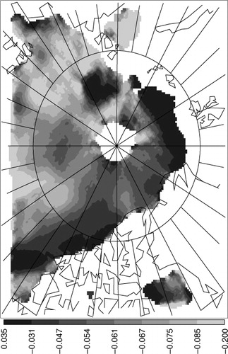
Figure 8 shows the bias between the OSI SAF and the dynamical method emissivities. The bias is from −0.19 to 0.04, with a tendency for the dynamical method to have higher emissivities over first-year ice than the OSI SAF model. In fact, the dynamical method emissivities are systematically greater than 1 in some of the areas covered by first-year ice.

Fig. 8.  Map of mean emissivity difference between the OSI SAF method and the dynamic method (from NOAA-15 for the 2-month-period, 1 November to 31 December 2011). Latitude and longitude lines are shown for every 10° south of 80°N, and the −90 Meridian is vertical.

5.2 Comparison of observed and simulated brightness temperatures using RTTOV-8 and HIRLAM

The OSI SAF emissivity is used in a forward radiative transfer calculation for estimating brightness temperatures at the sounding channels near 50 GHz. This estimate is then compared to observations.

When assimilating sounding data, there are systematic errors in the forward model. These systematic errors can partly be removed by a bias correction procedure. Our bias correction uses standard statistical regression on a dataset of observations and corresponding simulated observations to find an optimal correction to the observations. Here, this correction is static and applies a set of predictors affecting the errors. We first tried to compare the match between observed and simulated brightness temperatures without any bias correction. It turned out to produce quite large scatter, which was expected. However, it was difficult to interpret the results. Instead we have implemented the bias correction scheme to correct the observations before analysing the correlation.

The surface air temperature is available in HIRLAM. However, because of penetration into the snow and ice, the surface temperature is not synonymous with the microwave effective temperature. The effective temperature (T _eff ) is higher than the 2 m air temperature (T _air ) and the surface temperature during winter. Mathew et al. (2008) uses a linear relation, that is, T _eff =a*T _air +b, where a is the slope and b is the offset. Alternatively, it has been proposed to use the snow ice interface temperature (Tonboe et al., 2011). This would lead to a similar relation. Here, we use the surface temperature as a predictor in the bias correction. This yields a correction with linear coefficients determined implicitly from the dataset rather than being predetermined as in Mathew et al. (2008) and in Tonboe et al. (2011), and this makes the bias correction physically meaningful. In addition to surface temperature, scan angle, scan angle squared and thickness (vertically averaged temperature) of several atmospheric layers were used as predictors in the bias correction. Separate bias correction coefficients were derived for the OSI SAF model and for the tie-point model.

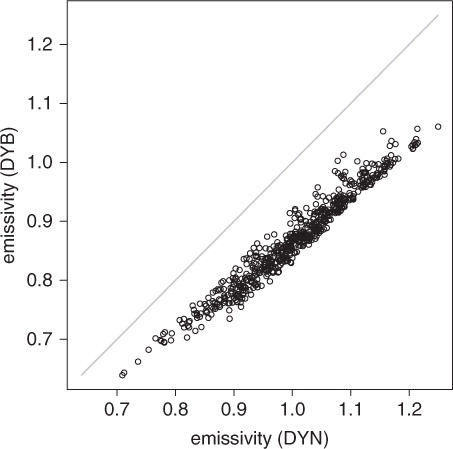
When investigating the fit between simulated data and observations for the dynamical method, we have not derived a separate bias correction but have used the bias coefficients from the OSI SAF model. This is because we expected that a prior bias correction would make the emissivity derived with the dynamical method from AMSU channel 3 (50.3 GHz) more physically realistic. Figure 9 shows the emissivity derived with the dynamical method with and without bias correction. The bias correction reduces the number of unphysical emissivities greater than one. Therefore, in the following we will only show results from the dynamical method based on bias corrected data.

Fig. 9.  Comparison between emissivities calculated using the dynamical method using bias corrected brightness temperatures on the vertical axis (emissivity DYB) and calculations using raw uncorrected brightness temperatures on the horizontal axis (emissivity DYN). NOAA-15, period 1 November to 31 December 2011.

The geographical distribution of average observed minus simulated brightness temperatures for channel 5 using the OSI SAF model is shown in Fig. 10. We see a large scale pattern across the Arctic with negative values in the multiyear ice area North of Greenland indicating overestimation of the OSI SAF emissivities in this area and vice versa in areas covered by first-year ice. In Fig. 11, we show the corresponding standard deviation of departures between the OSI SAF model and the observations. The variability is smaller over areas covered by multiyear ice than areas covered by new- and first-year ice. It is expected that the emissivity variability is higher in areas where ice is forming and signatures are changing more rapidly than in areas with perennial ice.

Fig. 10.  Map mean departure of observed minus simulated brightness temperatures [K] for channel 5 (from NOAA-15 for the 2-month period; 1 November to 31 December 2011). Latitude and longitude lines are shown for every 10° south of 80°N.

Fig. 11.  Map of standard deviations of departures of observed minus simulated brightness temperatures [K] for channel 5 (from NOAA-15 for the 2-month period; 1 November to 31 December 2011 as above). Latitude and longitude lines are shown for every 10° south of 80°N.

Figure 12 shows the correlation between simulated and observed AMSU brightness temperatures for channel 4. The scatter plots in Fig. 12A show the fit for the tie-point model and the OSI SAF model is shown in Fig. 12B. Channel 4 (52.8 GHz) is dominated by surface emission and it has largest scatter between observed and simulated emissivities indicating that there is a significant uncertainty in determining the surface emission. For channels 5–7, which are dominated by atmospheric emission, the correlation is higher as summarised in Table 1. In general, there is higher correlation with the OSI SAF model than with the tie-point model.

Fig. 12.  The measured and bias corrected AMSU-A channel 4 brightness temperatures (Tb [K] observation) versus the brightness temperature predicted with (A) RTTOV-8 and the OSI SAF model (Tb [K] simulation – OSI SAF); (B) RTTOV-8 and the tie-point model (Tb [K] simulation-tie-point). Bias correction was done towards modelled data applying the OSI SAF model.

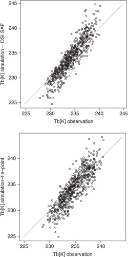
Table 1. Standard deviation of departures [K] between the simulated AMSU-A measurements using the tie-point and the OSI SAF emissivity models and bias corrected observations

	NOAA-15 tie-point model	NOAA-15 OSI SAF model	NOAA-16 tie-point model	NOAA-16 OSI SAF model
Ch. 3 (50.3 GHz) [K]	5.58	3.94	5.45	3.98
Ch. 4 (52.8 GHz) [K]	1.76	1.54	–	–
Ch. 5 (53.3 GHz) [K]	0.66	0.63	0.65	0.63
Ch. 6 (54.4 GHz) [K]	0.24	0.24	0.22	0.21
Ch. 7 (54.9 GHz) [K]	0.20	0.20	0.27	0.27

The two columns to the left are for NOAA-15, the two to the right for NOAA-16. Note that channel 4 on NOAA 16 is not operational.

In Table 2, the fit between observations and simulations of the OSI SAF model is compared to the fit between observations and simulations using the dynamical method. For the channels where the surface emission is dominant, the fit with the dynamical method is better. However, the OSI SAF model becomes comparable for channels where the atmospheric contribution is dominant. It is not unexpected or an indication of poor performance of the OSI SAF model that the dynamical method gives a better fit than the OSI SAF model to the channels dominated by the surface.

Table 2. Standard deviation of departures in [K] between the simulated AMSU-A measurements with the OSI SAF emissivity model and bias corrected observations

	NOAA-15 Dynamical method	NOAA-15 OSI SAF model	NOAA-16 Dynamical method	NOAA-16 OSI SAF model
Ch. 3 (50.3 GHz) [K]	0	3.95	0	3.98
Ch. 4 (52.8 GHz) [K]	0.86	1.54	–	–
Ch. 5 (53.3 GHz) [K]	0.53	0.63	0.56	0.63
Ch. 6 (54.4 GHz) [K]	0.23	0.24	0.22	0.21
Ch. 7 (54.9 GHz) [K]	0.20	0.20	0.27	0.27

The two columns to the left are for NOAA-15, the two to the right for NOAA-16. Note that channel 4 on NOAA 16 is not operational.

The dynamical method adjusts the emissivities to make the simulated emissivities fit the observations in channel 3 using the HIRLAM data in the forward calculation. However, an inaccuracy in the emissivities is only one of several reasons which can cause misfit between observations and simulations as discussed in section 5. This means that the emissivity estimate from the dynamical method will make the observations fit even if there are other variables than surface emissivity contributing to the signal. These other contributions are potentially representativeness errors or other observation errors. This can explain the fact that emissivities greater than 1 are seen in Fig. 7B, where emissivities were derived with the dynamical method. If the dynamical method compensates this type of observation uncertainty, it could be regarded as an asset, if these errors in channel 3 were correlated to other channels. However, if there is no correlation of the uncertainty between different channels, the methodology may just be introducing new errors in neighbouring channels.

The primary contribution to the signal is from the surface in the AMSU channel 3 (50.3 GHz). However, there is also a small contribution to the signal from the atmosphere and therefore the emissivity estimate from the dynamical method is adjusted to compensate if there are errors in the lower part of the atmospheric profile from HIRLAM. It is the signal from the lower part of the troposphere we wish to exploit in the NWP data assimilation. Because the same atmospheric signal also affects the brightness temperature in other lower-tropospheric channels using the same simulated emissivity there is a risk that part of the good fit using the dynamical method is obtained by neglecting the atmospheric signal that we are interested in.

It is therefore encouraging that the fit with the OSI SAF method, which provides an independent estimate, is comparable or better than the dynamical method for channels dominated by atmospheric emission.

6. Conclusions

The OSI SAF model is applicable to both the AMSU and the SSMIS sounders. The model estimates the 50 GHz vertically and horizontally polarised emission at incidence angles between nadir and 60° as a function of GR1836 and PR36, which is measured by SSMIS. Under the assumption of near zero, 3rd and 4th Stokes parameters the polarisation at different incidence angles on AMSU is a mix between the vertical and horizontal polarisation. On SSMIS the emissivity can be estimated using the same viewing geometry as on its sounding channels.

The geographic variability of the emissivity is high with nadir emissivities on the northern hemisphere between 0.7 and 0.95 and on the southern hemisphere between 0.6 and 0.96. On the northern hemisphere there are large differences between first- and multiyear ice types. On the southern hemisphere, the variability is presumably caused by different snow cover conditions. The polarisation parameter, R, is between 0.2 and 0.4 in the Arctic and between 0.2 and 0.5 around Antarctica. The R parameters indicate the level of specularity where completely specular for R=1 is a level ice surface with a permittivity of 3.5, and the polarisation is determined by the Fresnel reflection coefficients. The scattering is diffuse when R=0. Diffuse emission is uniform and independent of incidence angle and polarisation.

The OSI SAF emissivity is compared to the emissivity estimated with the tie-point model. The first-year ice emissivities using the two models are comparable. However, multiyear ice emissivity is higher using the tie-point model than the OSI SAF model. Multiyear ice emissivities from the literature compare closer with the OSI SAF model than the tie-point model.

The OSI SAF emissivity is input to RTTOV-8 for simulating the surface contribution to the near 50 GHz sounding channels using additional atmospheric profiles from HIRLAM. The bias between the two estimates is small but there is a high variability. The high variability is caused by real differences in the surface emissivity estimates and imperfections in the simulated atmospheric profiles and the surface effective temperature. The OSI SAF model has the advantage compared to the dynamical method that it is independent of the AMSU measurements used for atmospheric sounding. Therefore, the risk of confusing atmospheric emission with the surface emission when using the OSI SAF model is lower than when using the dynamical method for AMSU sounding data assimilation. Even if the fit with the AMSU-A observations seen with the OSI SAF model is good, it is not given that it necessarily is producing better results than other methods when applied in data assimilation. We have mentioned the issues with the dynamical method compensating observation errors and partly absorbing the atmospheric signal. This can only be verified by performing full impact studies with the NWP system. However it is likely that the better fit of the OSI SAF emissivity model is also better for assimilation, because the emissivity has been derived with a method that is independent from the atmospheric profiles within the NWP model.

Actual validation of the model is difficult on satellite foot-print scale. However, for a more complete assessment of the model there are a number of issues for future investigation: 1) to perform a numerical weather prediction assimilation experiments with sounding data comparing the different emissivity models impact on forecast skill, 2) to assess the importance of the sea ice emissivity vs. the effective temperature and the threshold accuracy for both parameters, 3) to extend sea ice emissivity evaluation to include both winter and summer and to the southern hemisphere and 4) conduct measurement campaigns in the field for model validation and for tuning of the model coefficients.

7. Acknowledgements

This study was supported by EUMETSAT's Ocean and Sea Ice Satellite Application Facility and the Greenland Climate Research Centre.

References

- Aires, F, Prigent, C, Bernardo, F, Jimenez, C, Saunders, R. and co-authors. 2010. A tool to estimate land surface emissivities at microwaves frequencies (TELSEM) for use in numerical weather prediction. Q. J. Roy. Meteor. Soc. 137, 690–699. DOI: 10.3402/tellusa.v65i0.18380.
- Comiso J. C. Cavalieri D. J. Parkinson C. L. Gloersen P. Passive microwave algorithms for sea ice concentration: a comparison of two techniques. Remote Sens. Environ. 1997; 60: 357–384. 10.3402/tellusa.v65i0.18380.
- Drusch, M, Holmes, T, de Rosnay, P and Balsamo, G. 2009. Comparing ERA-40 based L-band brightness temperatures with skylab observations: a calibration/validation study using the community microwave emission model. J. Hydrometeorol. 10, 213–226. DOI: 10.3402/tellusa.v65i0.18380.
- English S. J. The importance of accurate skin temperature in assimilating radiances from satellite sounding instruments. IEEE T. Geosci. Remote. 2008; 46(2): 403–408. 10.3402/tellusa.v65i0.18380.
- Harlow R. C. Sea ice emissivities and effective temperatures at MHS frequencies: an analysis of airborne microwave data measured during two Arctic campaigns. IEEE T. Geosci. Remote. 2011; 49(4): 1223–1237. 10.3402/tellusa.v65i0.18380.
- Heygster, G, Melsheimer, C, Mathew, N, Toudal, L, Saldo, R. and co-authors. 2009. POLAR PROGRAM: integrated observation and modeling of the Arctic sea ice and atmosphere. B. Am. Meteorol. Soc. 90, 293–297. 10.3402/tellusa.v65i0.18380.
- Karbou F. Gérard E. Rabier F. Microwave land emissivity and skin temperature for AMSU-A & -B assimilation over land. Q. J. Roy. Meteor. Soc. 2006; 132(620): 2333–2355. 10.3402/tellusa.v65i0.18380.
- Karbou F. Rabier F. Lafore J.-P. Redelsperger J.-L. Bock O. Global 4DVAR assimilation and forecast experiments using AMSU observations over land. Part II: Impacts of assimilating surface sensitive channels on the African monsoon during AMMA. Weather. Forecast. 2010; 25: 20–36. 10.3402/tellusa.v65i0.18380.
- Kongoli C. Boukabara S.-A. Yan B. Weng F. Ferraro R. A new sea-ice concentration algorithm based on microwave surface emissivities – application to AMSU measurements. IEEE T. Geosci. Remote. 2011; 49(1): 175–189. 10.3402/tellusa.v65i0.18380.
- Kunkee, D. B, Poe, G. A, Boucher, D. J, Swadley, S. D, Hong, Y. and co-authors. 2008. Design and evaluation of the first special sensor microwave imager/sounder. IEEE T. Geosci. Remote. 46(4), 863–883. 10.3402/tellusa.v65i0.18380.
- Mathew N. Heygster G. Melsheimer C. Kaleschke L. Surface emissivity of Arctic sea ice at AMSU window frequencies. IEEE T. Geosci. Remote. 2008; 46(8): 2298–2306. 10.3402/tellusa.v65i0.18380.
- Mätzler C. On the determination of surface emissivity from satellite observations. IEEE Geosci. Remote S. 2005; 2(2): 160–163. 10.3402/tellusa.v65i0.18380.
- Mätzler, C, Rosenkranz, P. W, Battaglia, A. and Wigneron, J. P. 2006. Thermal Microwave Radiation – Applications for Remote Sensing. IEE Electromagnetic Waves Series: London.
- Mo T. Prelaunch calibration of the advanced microwave sounding unit-A for NOAA-K. IEEE T. Microw. Theory. 1996; 44(8): 1460–1469. 10.3402/tellusa.v65i0.18380.
- Narvekar P. S. Heygster G. Tonboe R. Jackson T. J. Analysis of WindSat third and fourth stokes components over Arctic sea ice. IEEE T. Geosci. Remote. 2011; 49(5): 1627–1636. 10.3402/tellusa.v65i0.18380.
- Patterson, T. 2010. SSMIS SDR BUFR Format. EUM/OPS/TEN/10/1665, EUMETSAT.
- Saunders R. W. Matricardi M. Brunel P. An improved fast radiative transfer model for assimilation of satellite radiance observations. Q. J. Roy. Meteor. Soc. 1999; 125: 1407–1425.
- Thyness, V. W, Toudal Pedersen, L, Schyberg, H and Tveter, F. T. 2005. Assimilating AMSU-A over Sea Ice in HIRLAM 3D-Var. In: ITSC XIV Proceedings. BeijingChina.
- Tonboe, R. T. 2005. A mass and thermodynamic model for sea ice. Danish Meteorological Institute Scientific Report 05–10, p. 12.
- Tonboe R. T. The simulated sea ice thermal microwave emission at window and sounding frequencies. Tellus A. 2010; 62: 333–344. 10.3402/tellusa.v65i0.18380.
- Tonboe R. T. Dybkjær G. Høyer J. L. Simulations of the snow covered sea ice surface temperature and microwave effective temperature. Tellus A. 2011; 63: 1028–1037. 10.3402/tellusa.v65i0.18380.
- Ulaby, F. T, Moore, R. K and Fung, A. K. 1982. Microwave remote sensing, active and passive. Vol. II, Artech House: Norwood MA.
- Ulaby, F. T, Moore, R. K and Fung, A. K. 1986. Microwave remote sensing, active and passive. Vol. III, Artech House: Norwood MA.
- Weng F. Yan B. Grody N. C. A microwave land emissivity model. J. Geophys. Res. 2001; 106(D17): 20115–20123. 10.3402/tellusa.v65i0.18380.
- Wiesmann A. Mätzler C. Microwave emission model of layered snowpacks. Remote Sens. Environ. 1999; 70(3): 307–316. 10.3402/tellusa.v65i0.18380.
- Willmes S. Haas C. Nicolaus M. High radar-backscatter regions on Antarctic sea-ice and their relation to sea-ice and snow properties and meteorological conditions. Int. J. Remote Sens. 2011; 32(14): 3967–3984. 10.3402/tellusa.v65i0.18380.