Non-linear forcing singular vector of a two-dimensional quasi-geostrophic model

ABSTRACT

We propose a non-linear forcing singular vector (NFSV) approach to infer the effect of non-linearity on the predictability associated with model errors. The NFSV is a generalisation of the forcing singular vector (FSV) to non-linear fields and acts as a tendency perturbation that results in a significantly large perturbation growth. In predictability studies, the NFSV, as a tendency error, may provide useful information about model errors that cause severe prediction uncertainties. In this article, a two-dimensional quasi-geostrophic (QG) model is used to study NFSVs and make a comparison between NFSVs and FSVs. We choose two basic flows: the first is a zonal steady flow (Ref-1), and the second is a meridional steady flow (Ref-2). The results demonstrate that the corresponding NFSVs contain a phase where the stream function tends to be contracted around regions of strong velocity shear. Furthermore, the NFSVs for the Ref-1 tend to have a meridional asymmetric spatial structure. Due to the absence of non-linearity, FSVs tend to have a larger spatial extension than NFSVs; in particular, the FSVs for the Ref-1 are almost symmetric in the stream function component. The prediction errors caused by FSVs in the non-linear QG model are generally smaller than those caused by FSVs in the linearised QG model; therefore, the non-linearity in the QG model would significantly saturate the perturbation growth. Nevertheless, the prediction errors caused by NFSVs (especially for the Ref-1) in the non-linear QG model are larger than those caused by FSVs, which further implies that the tendency errors of NFSV structures tend to reduce the damping effect of the non-linearity on the perturbation growth and are more applicable than those of FSV structures to describing the optimal mode of the model errors. The differences between NFSVs and FSVs demonstrate the usefulness of NFSVs in revealing the effects of non-linearity on predictability. The NFSV may be a useful non-linear technique for exploring the predictability problems introduced by model errors.

• weather
• climate
• predictability
• model error
• optimal perturbation

1. Introduction

One of the central problems in atmospheric and oceanic sciences is weather and climate predictability, in which estimating the uncertainties associated with the predictions is very important. Tennekes (1991) proclaimed that no forecast was complete without an estimate of the prediction error. Since this perspective was first proposed by Thompson (1957), operational weather forecasting has progressed to making explicit attempts to quantify the evolution of the initial uncertainty during each forecast (Palmer et al., 1992; Toth and Kalnay, 1997; Mu et al., 2003). Some understanding of the predictability for tropical ocean-atmosphere system has also been gained by studying the growth of errors and uncertainties during forecasting (Moore and Kleeman, 1996; Samelson and Tziperman, 2001; Mu et al., 2007a, 2007b).

Prediction uncertainties are generally caused by initial errors and model errors. To study the roles of initial errors and model errors in yielding prediction uncertainties, Lorenz (1975) classified two types of predictability problems: the first is related to initial errors and assumes a perfect model, whereas the second is associated with model errors and assumes a perfect initial field. The former has been largely explored, resulting in the proposal and introduction of many theories and methods in which optimal methods are important for estimating the predictability limit of weather and climate (Lorenz, 1965; Toth and Kalnay, 1997; Mu et al., 2003; Riviere et al., 2008). In this context, the singular vector (SV) approach was first introduced in meteorology (Lorenz, 1965; Farrell, 1989). Considering the limitations of the linear theory of SV, Mu et al. (2003) proposed the conditional non-linear optimal perturbation approach (CNOP) to search for the optimal initial perturbation for a given constraint; the competing aspect of this approach is that it sufficiently considers the effect of non-linearity. CNOP has been applied to weather and climate predictability studies (Duan et al., 2004; Mu et al., 2004; Duan and Mu, 2006; Mu et al., 2007a, 2007b; Duan et al., 2008; Terwisscha and Dijkstra, 2008; Duan et al., 2009; Jiang and Mu, 2009; Mu et al., 2009; Wu and Mu, 2009). Recently, Riviere et al. (2009) demonstrated an extension of the CNOP approach and used it to estimate the predictability of atmospheric moisture processes in an attempt to reveal the effects of non-linear processes. Oortwijn and Barkmeijer (1995) and Barkmeijer (1996) also realised the limitations of the linear technique and considered non-linear effects using an iterative procedure. The bred vector (Toth and Kalnay, 1997) is another important non-linear optimal method that was generalised from the Lyapunov vector approach and has been used to investigate the first type of climate predictability problem (Cai et al., 2003). All of these theories and methods have played important roles in guiding scientists to develop and improve numerical models and propose innovative ideas to increase the accuracy of weather and climate forecasts (Houtekamer and Deroma, 1995; Xue et al., 1997; Thompson, 1998; Hamill et al., 2000; Mu and Zhang, 2006; Mu et al., 2009).

The existing numerical models cannot yet accurately describe atmospheric and oceanic motions. Uncertainties in the parameterisation of subgrid-scale physical processes, external forcing, and numerical discrete schemes, etc., may result in model errors. Substantial progress has been achieved in improving the quality of forecasts during the last few decades (Simmons and Hollingsworth, 2002); however, these factors will always limit forecast accuracy and should be considered during forecasting (Houtekamer et al., 1996; Buizza et al., 1999; Mylne et al., 2002). Studies of model errors are related to the second type of predictability problem (Lorenz, 1975). It is important to estimate the predictability limit caused by model errors. Mu et al. (2010) extended the CNOP approach to investigate the optimal mode of model parameter uncertainties and estimated the predictability limit introduced by model parameter errors. Roads (1987) used constant tendency errors to approximate model uncertainties. A procedure has been developed to compute the time-independent forcing of model tendencies based on observed fields (Roads, 1987). By writing the model in the form1.1

where F( U ( x ; t)) is the total model tendency, the forcing f is computed by inserting the observed fields for x. The forcing term f as defined by Roads’ procedure can be interpreted as a crude method to account for processes that are not explicitly or correctly described by the model equations (Roads, 1987; Barkmeijer et al., 2003). Following this reasoning, Moore and Kleeman (1999) developed an approach, called the (linear) stochastic optimal approach, to study the ENSO predictability limit caused by model errors. However, Barkmeijer et al. (2003) thought that the stochastic optimal approach was not feasible in a realistic high-dimensional numerical model because of the explicit matrix computation of the linear model propagator and its adjoint. To compensate for this limitation of the stochastic optimal approach, Barkmeijer et al. (2003) proposed the concept of the (linear) forcing singular vector (FSV), which is constant in time but represents the tendency perturbation leading to a significantly large perturbation growth in a linearised model during a given forecast period (Barkmeijer et al., 2003). D'Andrea and Vautard (2000) studied similar structures as a way to reduce the systematic error in a quasi-geostrophic (QG) model. Farrell and Ioannou (2005) further determined the optimal set of the distributed deterministic and stochastic forcings in the forecast and observer systems over a chosen time interval, also based on a linear system.

The motions of the atmosphere and ocean are generally governed by complex non-linear systems. The FSV is derived by the linear approximation of a non-linear model (the linearised model), which raises concerns about the validity of the linearised model. That is, how can the linearised model approximation to its non-linear counterpart be validated in advance? Some papers have attempted to address this concern, but very few satisfying answers have been found (Lacarra and Talagrand, 1988; Tanguay et al., 1995). Therefore, it is desirable and often necessary to address non-linear models rather than their linear approximations in numerical weather and climate prediction. Therefore, this article investigates the FSV approach within the frame of a non-linear model.

This article is organised into five sections. In section 2, a non-linear forcing singular vector (NFSV) is proposed. The NFSV calculation is discussed in section 3. In section 4, we study the NFSVs of a two-dimensional QG model and investigate the differences between NFSVs and FSVs and illustrate the usefulness of NFSVs in revealing the effects of non-linearity. Finally, the results obtained in this study are summarised, and the physical interpretations of the NFSV are discussed in section 5.

2. Non-linear forcing singular vector

We write the evolution equations for the state vector U , which may represent the surface current, thermocline depth, and sea surface temperature, etc., as follows:2.1

where U ( x , t)=( U ₁( x , t), U ₂( x , t), ···, U _n ( x , t)); U ₀ is the initial state; ( x , t)∈Ω×[0,τ], in which Ω is a domain in R ⁿ , x =(x ₁, x ₂, ···, x _n ) and t is the time; and τ<+∞ is the final time of the state variables evolution. F is a non-linear operator. Assuming that the dynamical system equation [eq. (2.1)] and the initial state are known exactly, the future state can be determined by integrating eq. (2.1) using the appropriate initial conditions. The solution to eq. (2.1) for the state vector U at time τ is given by2.2

Here, M _τ is the propagator of eq. (2.1) and ‘propagates’ the initial value to the prediction time τ as described by eq. (2.2).

In realistic predictions, forecast systems generally contain both initial errors and model errors. In predictability studies, initial errors are often measured by perturbations superimposed on the initial fields of the numerical model. For model errors, Roads (1987), Moore and Kleeman (1999), and Barkmeijer et al. (2003) used a tendency perturbation to investigate the effects of model errors on the prediction results. Furthermore, Barkmeijer et al. (2003) considered a constant tendency perturbation and developed the FSV approach to study the predictability problems associated with model errors.

We describe forecast models with initial perturbations and constant tendency perturbations as in eq. (2.3).2.3

We use M _τ ( f ) to denote the propagator of eq. (2.3). In fact, M _τ ( f ) with f =0 is the same as M _τ in eq. (2.2), i.e. the propagator of eq. (2.1). Then, we obtain2.4

where U ( x ,τ)=M _τ (0)( U ₀)=M _τ ( U ₀). From eqs. (2.2) and (2.4), it is easily derived that u ^I _f ( x ,τ)=M _τ ( f )( U ₀+ u ₀)−M _τ ( U ₀), which describes the departure from the state U ( x ,τ) [i.e. M _τ ( U ₀)] caused by the initial perturbation u ₀ and constant tendency perturbation f . In the scenario describing the first type of predictability problem, the model is thought to be perfect. In this case, the constant tendency perturbations (as model systematic errors) are equal to zero (i.e. f =0), and the situation in which M _τ (0)( U ₀+ u ₀)= U ( x ,τ)+ u ^I ( x , t), where u ^I ( x , t) represents the evolution of initial errors u ₀, is considered. For the second type of predictability problem, the initial fields are assumed perfect (i.e. the initial errors u ₀=0), and M _τ ( f )( U ₀)= U ( x ,τ)+ u _f ( x ,τ) is of interest. Then, u _f ( x ,τ) describes the departure from the state U ( x ,τ) caused by the constant tendency perturbation (i.e. constant tendency error) f , which may describe a type of model systematic error.

Barkmeijer et al. (2003) considered the linearised version of a non-linear model. The perturbation equation for the non-linear model eq. (2.1) can be obtained by subtracting eq. (2.1) from eq. (2.3). By omitting the non-linear term, a linearised perturbation equation is obtained:2.5

where u ₀, u , and U have the same meanings as in eq. (2.3), and F( U ) is the Jacobian of the non-linear operator F with respect to the reference state U ( x , t ). With the constant tendency perturbation f ( x ), the FSV f ^* can be obtained by solving the linear optimisation problem of eq. (2.6).2.6

where the norm is described by the inner product , and M _τ is the propagator of eq. (2.5) and is equivalent to the tangent linear operator of the non-linear propagator M _τ ( f ) of eq. (2.3).

It is clear from eq. (2.6) that the FSV is derived from a linear model. Next, we generalise the FSV to a non-linear field and propose a non-linear technique of FSV to determine the effects of non-linearity on the predictability limit caused by the model uncertainties. As mentioned in the introduction, Mu et al. (2010) extended the CNOP approach to investigate the model parameter perturbations (CNOP-P) that cause the largest prediction error. It is inferred that if we express the constant tendency perturbation as external parameters that display a certain spatial structure, we can use the CNOP-P technique to derive the non-linear FSV.

For a chosen measurement, a tendency perturbation is defined as a non-linear FSV (NFSV) if and only if2.7

where2.8

M _τ ( f ) is the propagator of the non-linear model, eq. (2.3), and , which is defined by the norm , is the constraint condition of the tendency perturbation f . The objective function J with the norm measures the magnitude of the departure from the reference state M _τ (0)( U ₀) caused by the tendency perturbation f . We note that the norms and represent different norms. In some situations, the norm can be the same as depending on the physical problem being investigated. As mentioned in the introduction, Roads (1987) proposed a procedure to compute a time-independent forcing of model tendencies based on observation fields, and this motivates a similar approach to compute the allowable magnitudes of the constant tendency perturbation before determining the constraint condition amplitude (i.e. δ). Because this article is focused on methodology, to illustrate the NFSV approach, we experimentally choose the amplitudes of the constraint conditions to calculate the NFSVs.

Eq. (2.7) is a constrained maximisation problem. By solving this optimisation problem, one can obtain the NFSV, . It is easily shown from eqs. (2.7) and (2.8) that the function J, which is associated with the NFSV, measures the magnitude of the departure of the reference state M _τ (0)( U ₀) caused by the constant tendency perturbation. Furthermore, the function requires us to find the constant tendency perturbation that causes the greatest departure from the reference state M _τ (0)( U ₀) at a future time τ _. Then, the constant tendency perturbation of the NFSV pattern introduces the greatest departure from the reference state M _τ (0)( U ₀) at a future time τ in terms of the chosen measurement norm. In other words, the NFSV induces the largest perturbation growth at the given future time τ _. In predictability studies, the NFSV , as a constant tendency error, may represent a type of model systematic error that causes a significantly large prediction error at the prediction time.

We notice that the NFSV defined by eq. (2.7) is established on the assumption that the tendency perturbation does not change with time. Therefore, in predictability studies, the tendency errors are assumed to be constant in time. However, realistic tendency errors may be time-dependent; thus, it is necessary to generalise the constant NFSV to be time-dependent. Actually, using the constant NFSV, we can derive a time-dependent NFSV. For the time steps , a time-dependent NFSV can be obtained by the following optimisation problem:2.9

where is the propagator of eq. (2.3) from time t _i to t _i+1 and _. From eq. (2.9), it is easily observed that the time-dependent NFSVs can be obtained by computing several constant NFSVs. Considering that the FSV is constant (see Barkmeijer et al., 2003) and that the goal of this article is to reveal the differences between FSV and NFSV, we only study the constant NFSVs and explore the effects of non-linearity on the optimal tendency perturbation.

3. Computing the non-linear forcing singular vectors

The NFSV is related to a constrained optimisation problem. It is very difficult to solve such optimisation problems analytically; therefore, we have to solve it numerically. Such optimisation problems are often solved using optimisation algorithms, where the gradient of the related objective function is very important. During large-scale optimisation, the gradient of the objective function with respect to the initial perturbations is often obtained using the adjoint method (Le Dimet and Talagrand, 1986). For example, Mu et al. (2003) proposed the CNOP approach, which is characterised by an optimisation problem, and computed the CNOP along the gradient direction of the objective function, where the gradient is derived using an adjoint method. Although the NFSV can also be solved using an adjoint method, computing the NFSV requires the gradient of the objective function with respect to the constant tendency perturbation f . In fact, the gradient of the objective function with respect to the tendency perturbation f can be transferred to a particular case of the objective function with augmented initial perturbations. Next, we describe how to compute the NFSVs using a gradient.

Existing optimisation solvers are often used to compute minimisation problems; however, the NFSV is related to a constrained maximisation problem. To calculate the NFSVs, we convert the maximisation problem to a minimisation problem. In particular, we rewrite eq. (2.8) as follows:3.1

where u _f (τ) is a departure from the reference state U ( x ,τ)=M _τ (0)( U ₀) caused by the constant tendency perturbation f , and is the inner product. To facilitate the description, we will use u (τ) instead of u _f (τ). The maximisation problem (2.7) related to the NFSVs then becomes a minimisation problem of the function J ₁( f ).

The first-order variation of J ₁( f ) is as follows:3.2

Furthermore, δf is governed by the following tangent linear model:3.3

By introducing two Lagrangian multipliers, λ ₁ and λ ₂, we obtain3.4

By solving eq. (3.4) (details are found in the Appendix) and comparing it with eq. (3.2), we obtain the following gradient:3.5

λ ₁(t) and λ ₂(t) in eqs. (3.4) and (3.5) satisfy3.6

and eq. (3.6) is the adjoint equation of eq. (3.3). By integrating eq. (3.6), we obtain the gradient and thereby allow the NFSV to be computed using optimisation solvers such as Spectral Projected Gradient 2 (SPG2; Birgin et al., 2000), Sequential Quadratic Programming (SQP; Powell et al., 1982), and Limited Memory Broyden-Fletcher-Goldfarb-Shanno (L-BFGS; Liu and Nocedal, 1989).

From eq. (3.6), it is clear that λ ₁(0) is necessary to obtain the gradient λ ₂(0). From eq. (3.5), we know that λ ₁(t) satisfies the equation3.7

It is clear that eq. (3.7) is composed of the adjoint model of the non-linear model, eq. (2.1), with respect to the initial perturbations. Therefore, the adjoint model in eq. (3.6), which is associated with the constant tendency perturbation f , is based on eq. (3.7), which is associated with the initial perturbations. Numerically, we do not alter the existing adjoint model in eq. (3.7) but only add a line of code showing the discretisation of the equation with after the code of the adjoint model in eq. (3.7) to obtain the adjoint model in eq. (3.6). Several models have adjoint models with respect to the initial perturbations and have been used to solve the CNOP and linear singular vectors. For example, see the two-dimensional QG model used in this study, the three-layer QG model, the Zebiak-Cane model (Zebiak and Cane, 1987), and the Mesoscale Model 5 (Dudhia, 1993). Therefore, if one hopes to study the NFSVs of these models, one can easily modify the adjoint eq. (3.7) associated with the initial perturbations and then obtain the adjoint model in eq. (3.6), which is related to the NFSVs.

In this article, the gradient of the objective function J ₁ with respect to the initial perturbations and model perturbations is derived by introducing two Lagrangian multipliers, λ ₁ and λ ₂. This approach clearly shows the relationship between the adjoint model associated with initial perturbations and the adjoint model associated with the model perturbations, and this relationship helps us to numerically obtain the adjoint model associated with the constant tendency perturbations by modifying the existing adjoint models associated with the initial perturbations. Of course, the gradient can also be obtained by differentiating the objective function with respect to the initial perturbations and model perturbations (i.e. using the definition of the derivative of a non-linear operator) (see Shutyaev et al., 2008).

4. The NFSVs of a two-dimensional quasi-geostrophic model

We consider a two-dimensional QG model4.1

where P is the potential vorticity, Φ is the stream function, is the Laplacian operator, x and y are the zonal and meridional coordinates, t is the time, F is the planetary Froude number, f ₀ is the Coriolis parameter, H is the characteristic depth, and h _s is the topography. The horizontal Jacobian operator is shown as , and Ω=[0, X]×[0, Y] with a double periodical boundary condition. For any fixed T>0 and initial condition Φ₀, we can solve the initial value problem (4.1) to obtain Φ(x, y, T). Hence, the propagator M _τ is well defined; that is, is the solution to eq. (4.1) at a time T (see Mu and Zeng, 1991).

For eq. (4.1), we use a constant tendency error f(x, y) to disturb the model. The result is as follows:4.2

The propagator of the perturbed QG model eq. (4.2) is denoted by M _τ (f), where f is the tendency error of the model. Using this notation, the propagator M _τ in eq. (4.1) can be rewritten as M _t (0), which indicates that model eq. (4.1) is perfect. Following eq. (2.8), we write the objective function related to the NFSV as follows:4.3

where Φ₀ is the initial value of a basic flow. The norm is used to measure the effect of prediction errors caused by constant tendency errors f(x, y), where . The constraint conditions of the tendency errors f(x, y) is measured by the L ₂ norm, i.e. , where f _i,j represents the tendency errors at each space grid (i, j). The objective function J measures the magnitudes of the prediction errors caused by the constant tendency errors f(x, y) at time τ. The NFSVs obtained using eq. (4.3) represent the constant tendency errors that cause the largest prediction errors at the prediction time and describe a type of model systematic errors that induce severe prediction uncertainties.

To obtain the NFSV numerically, we use the discretisation versions of the operators M _τ (0) and M _τ (f). The Jacobian operator was discretised through the Arakawa finite difference scheme (cf. Arakawa, 1966). The temporal discretisation was carried out using the Adams-Bashforth scheme. The five-point difference scheme was employed to discretise the Laplacian operator. The stream function Φ is treated as an unknown term, and the potential vorticity P is calculated using the second equation from eq. (4.1). For an optimisation algorithm, we use the SPG2 method, which can be used to calculate the least value of a function of a large number of variables, subject to equality and inequality constraints. A detailed description of the algorithms can be found in Birgin et al. (2000).

To calculate the NFSVs using the SPG2 method, we made at least 30 initial random guesses; if several initial guesses for the SPG2 converge at a point in the phase space, this point can be considered as the maximum in a neighbourhood. Several such points are obtained. The point that maximises the objective function in eq. (2.8) is regarded as the NFSV. We note that the NFSV is the global maximum of the objective function J. However, it is possible that the objective function J attains its local maximum in the small neighbourhood of a point in the phase space. Such a tendency perturbation is called a local NFSV. In this study, we attempt to investigate the constant tendency error that causes the largest prediction error at the prediction time; therefore, we do not consider local NFSVs.

Based on the QG model, we study the NFSVs. Several non-linearly stable reference states (or basic flows) were used to investigate the NFSVs. The results demonstrate that the NFSVs depend on the given basic flows. In this article, we use two of the basic flows to describe the results associated with the NFSVs: one basic flow possesses the initial structure with a zonal flow (Ref-1) as in Fig. 1a and the other has a structure with an almost meridional flow (Ref-2) as in Fig. 1c. These two basic flows, as in Mu and Zhang (2006), are chosen based on Arnold's non-linear stability criteria (see Mu and Shepherd, 1994). A detailed description of these basic flows can be found in the Appendix to Mu and Zhang (2006). As a comparison, the FSVs of Ref-1 and Ref-2 are also computed by considering the tangent linear approximations M _t ( f ) and M _τ (0) of M _t ( f ) and M _τ (0) with respect to the given basic flows. To show the NFSVs and demonstrate the differences between the NFSVs and FSVs, two groups of comparisons are made. The first group of comparisons is concerned with the differences between the patterns of the NFSVs and FSVs, and the second is related to the differences between the prediction errors caused by the NFSVs and FSVs.

Fig. 1.  The stream function and the corresponding quasi-geostrophic winds of the Ref-1 and Ref-2 basic flows adopted in Experiments I and II, respectively. (a) and (b) correspond to the Ref-1 basic flow; (c) and (d) correspond to the Ref-2 basic flow.

We take the spatial domain of Ω=[0,6.4]×[0,3.2], which corresponds to the dimensional case [0,6400 km]×[0,3200 km]. The QG model parameters are chosen as follows: F=0.102, f ₀=10. The grid spacing d=0.2 corresponds to a dimensional length of 200 km, and the time step dt=0.006 corresponds to 10 min.

The NFSVs are a generalisation of the FSVs in a non-linear field and are required for a comparison with FSVs. The FSVs are derived from a linearised model as in eq. (2.4). It is easily shown that if f _L is an FSV, then a scaled vector cf _L (c is a constant) is also a FSV. We define a scaled FSV as follows:

thus,

That is, the scaled FSV possesses the same magnitude as that of the NFSV . Note that we are comparing NFSVs and FSVs.

4.1. A steady zonal basic flow

In this section, we choose a stable basic flow, which is obtained by integrating eq. (4.1) using the initial state . The relevant topography is , and 1/H=0.1. This basic flow is an equilibrium solution to eq. (4.1) and is denoted by ‘Ref-1’ (see Fig. 1). In the numerical experiments, the NFSVs are calculated for time steps 288, 720, 1008, and 1296, which correspond to the optimisation times (i.e. forecast periods) τ=2, 5, 7 and 9 d, respectively. The tendency perturbations f are experimentally constrained in with δ∈[0.8, 3.2]. In particular, we take δ=0.8, 1.6, 2.4 and 3.2 to describe the results.

4.1.1. Comparing the NFSVs and FSVs.

The computations demonstrate that for each optimisation time, there exists one NFSV of the Ref-1 for a given constraint magnitude. Figure 2 shows the stream function component of the NFSVs and the corresponding FSVs for the optimisation times of 2, 5, 7, and 9 d and a tendency perturbation magnitude (value of δ) of 1.6. The results show that the FSVs have a typical zonal wave number of 5 for all optimisation times and always show a symmetric V-shaped structure with concentrations around y=0.8 and y=2.4.

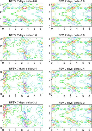
Fig. 2.  The stream function components of the NFSVs and FSVs of the Ref-1 basic flow with a perturbation magnitude of 1.6. The left (right) column lists the NFSVs (FSVs) with optimisation times of 2, 5, 7, and 9 d.

We note that the NFSVs have patterns similar to the FSVs only for short optimisation times (for example, the optimisation time τ=2 d) but are significantly different from the FSVs for long optimisation times (see Fig. 2). More precisely, NFSVs with long optimisation times compared to the FSVs have a very asymmetric V-shaped structure and cover a much smaller region, although they also tend to be concentrated around y=0.8 and y=2.4. The differences between the NFSV and FSV patterns depend not only on the optimisation times but also on the perturbation magnitudes. In Fig. 3, we plot the NFSV and FSV patterns with different magnitudes for the optimisation time of 7 d. The results show that the NFSVs are more similar to the FSVs for small tendency perturbations than for large tendency perturbations. That is, when the tendency perturbations are sufficiently small, the NFSVs tend to have a symmetric V-shaped structure similar to that of the FSVs, but when the tendency perturbations are large, the NFSVs become much more asymmetric. In summary, when the optimisation times are long and the tendency perturbations are large, the NFSVs tend to have a much more asymmetric region than the FSVs and cover a much smaller region.

Fig. 3.  The stream function components of the Ref-1 NFSVs and FSVs with an optimisation time of 7 d. The left (right) column lists the NFSVs (FSVs) with perturbation magnitudes of 0.8, 1.6, 2.4, and 3.2.

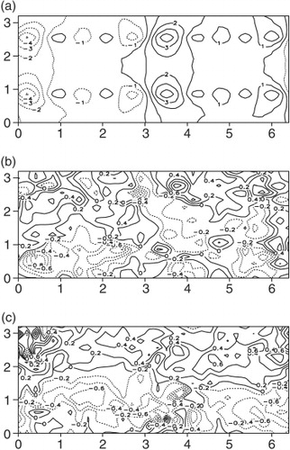
Figure 4 shows the patterns of the stream function components of the prediction errors caused by the NFSV and FSV obtained using an optimisation time of 7 d and a tendency perturbation magnitude of 1.6. The results show that the stream function component of the prediction error caused by the NFSV in the non-linear QG model is significantly different from that caused by the FSV. It is clear that the differences between the NFSV and FSV patterns also induce different responses in terms of the prediction errors at the prediction time. In particular, we find that the stream function components of the prediction errors caused by the NFSVs and FSVs in the non-linear QG model exhibit smaller-scale spatial patterns than those caused by the FSVs using the linearised model. Furthermore, some small-scale vortices can be observed in the stream function patterns of the prediction errors caused by the FSVs. All of these suggest that the small scales of the patterns result from the effects of the non-linearities.

Fig. 4.  Patterns of the stream functions of the prediction errors caused by (a) the FSV in the linearised QG model, (b) the FSV in the non-linear QG model, and (c) the NFSV in the non-linear QG model, where the optimisation is 7 d and the model perturbation magnitude is 1.6 in terms of the chosen norm.

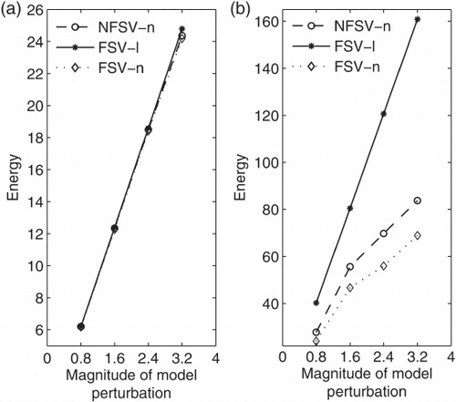
In addition, we also investigate the differences in the magnitudes of the prediction errors caused by the NFSVs and FSVs and find that the magnitudes of the prediction errors caused by the FSVs in the linearised QG model are larger than those caused by the FSVs in the non-linear QG model, especially for long optimisation times and/or large tendency perturbations (see Fig. 5). Thus, the non-linearity suppresses the linear growth of the prediction errors, i.e. the non-linearity has a damping effect on the growth of the prediction errors. Furthermore, we find that the prediction errors caused by the NFSVs in the non-linear QG model are larger than those caused by the FSVs in the non-linear QG model, indicating that the NFSVs of the asymmetric structure are inclined to reduce the non-linear damping effect on the error growth.

Fig. 5.  The prediction errors caused by the NFSVs and the FSVs in the QG model (denoted by NFSV-n and FSV-n) and those caused by the FSVs in the linearised QG model (denoted by FSV-l). The horizontal axis represents the perturbation magnitudes, and the vertical axis describes the prediction errors in terms of the energy. (a) uses an optimisation time of 2 d, and (b) uses the optimisation time of 7 d.

4.1.2. Interpretation.

The Ref-1 basic flow is zonal, and there is a strong velocity shear near y=0.8 and y=2.4, as the wind direction shifts from east to west near y=0.8 and from west to east near y=2.4 [see Fig. 1b]. Barotropic instabilities usually occur in regions with a strong velocity shear, and this condition may be favourable for the perturbations induced by the initial perturbations to extract energy from the basic flows (Pedlosky, 1979; Tung, 1981; Lacarra and Talagrand, 1988). We have shown that the FSVs and NFSVs that are expected to become large are concentrated around y=0.8 and y=2.4; therefore, the perturbations induced by the NFSVs and FSVs also tend to extract energy from the basic flow in regions with strong shear. In addition, Mak and Cai (1989) have demonstrated that a perturbation that has a phase tilted against the basic shear would optimally extract energy from the basic flow; this finding lends support to the assertion that the NFSVs and FSVs have V-shaped structures. Nevertheless, the NFSVs have much more asymmetric structures than the FSVs; furthermore, the NFSVs yield much larger prediction errors than the FSVs. Next, we will explain why the NFSVs of asymmetric structures cause larger prediction errors than the FSVs of symmetric structures.

We follow the Riviere et al. (2008), which shows that a shear opposite to the basic shear develops through time, to study the zonal mean of the stream function components of the prediction errors caused by the NFSVs and FSVs. In response, the growth rate of the instability (given by the total zonal-mean shear) should diminish (Gutowski, 1985; Nakamura, 1999; Riviere et al., 2008), and the perturbation will extract less energy from the basic flow. As a result, the growth of the prediction errors induced by the tendency errors will be limited. In Fig. 6, we illustrate the zonal-mean of the stream function component of the prediction errors caused by the NFSVs and FSVs with an optimisation time of 7 d and a tendency perturbation magnitude of 1.6. The figure shows that the zonal-mean shear induced by the NFSVs is weaker than that induced by the FSVs at the initial stage (e.g. at 2–5 d). It is inferred that the total zonal shear in the NFSV case is stronger than that in the FSV case, finally favouring the NFSVs to induce much larger prediction errors than the FSVs at the prediction time.

Fig. 6.  The zonal-means of the stream function of prediction errors (left column) and the corresponding zonal wind (right column) caused by (a, b) the FSV in the linearised QG model, (c, d) the FSV in the non-linear QG model, and (e, f) the NFSV in the non-linear QG model. The optimisation time is 7 d, and the model perturbation magnitude is 1.6.

We have demonstrated that the non-linearity has a damping effect on the growth of the prediction errors caused by the FSVs, and the tendency errors of the NFSV structures favour reducing the non-linear damping effect on the prediction errors and inducing larger prediction errors than the FSVs (see the last paragraph in section 4.1.1). In fact, the non-linearity here originates from the effect of perturbation advection in the non-linear QG model.

Assuming that the potential vorticity P with the corresponding stream function Φ is the basic flow of the QG model as mentioned in section 4.1.1, and the perturbation p with the corresponding stream function φ describes its prediction error caused by the tendency error f(x, y), then the evolution of the prediction error (p, φ) is described by the non-linear perturbation eq. (4.4).4.4

The linearised version of eq. (4.4) is given by eq. (4.5).4.5

It is noticed that eq. (4.5), compared to eq. (4.4), lacks the perturbation advection term , which is the non-linear term of the eq. (4.4). If p _N and p _L are the solutions of eqs. (4.4) and (4.5), respectively, p _N –p _L represents the effect of perturbation advection (or non-linear advection) on p _N . In this article, we are concerned with their corresponding stream function components ϕ _N and ϕ _L . Similarly, ϕ _N –ϕ _L describes the effect of non-linear advection on the evolution of the stream function ϕ _N .

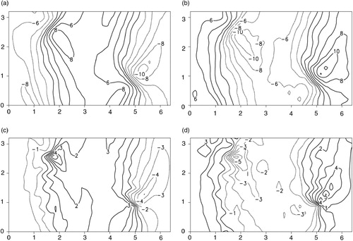
In Fig. 7b, we show the effect of the non-linear advection, which is indicated by ϕ _N –ϕ _L and associated with the tendency error FSV for an optimisation time of 7 d and a tendency perturbation magnitude of 1.6. It is shown that the vortices induced by the non-linear advection are concentrated around y=0.8 and y=2.4 and have vorticities of nearly opposite signs to those in the stream function components of the prediction errors caused by the FSVs in the linearised QG model [see Fig. 7a and 7b]. It is therefore inferred that, when the non-linear advection term is superimposed onto the linearised QG model, the vorticities associated with the prediction errors in the linearised QG model will be offset and the linear growth of the prediction errors induced by the FSV will then be suppressed by the non-linear advection. It follows that the non-linear advection has a damping effect on the growth of the prediction errors. In addition, we notice that the non-linear advection associated with the FSV shows an asymmetric effect in meridional direction [see Fig. 7b]. Therefore, despite the fact that the FSV is symmetric, the related non-linear advection has the ability to induce an asymmetric effect in the meridional direction; thus, the NFSVs resulting from the non-linear QG model exhibit an asymmetric mode. When the tendency error of the NFSV structure are forced to the non-linear QG model, the vortices induced by the non-linear advection also tend to have vorticities with opposite signs to those in the stream function components of the prediction errors caused by the NFSV in the linearised QG model and therefore suppress the perturbation growth [see Fig. 7c and 7d]. Furthermore, the NFSV, due to the effect of its spatial structure, induces the related non-linear advection to have smaller amplitude than the FSV case to suppress the perturbation growth. In other words, the tendency errors of the NFSV structure favour reducing the damping effect of non-linearity on the growth of the prediction errors and lead to larger prediction errors than the FSV. Another non-linear effect is that the non-linear advection tends to break the waves shown in the stream function patterns of the prediction errors caused by the NFSVs and FSVs and saturate them into much smaller scales (see Fig. 4; also see Riviere et al., 2008).

Fig. 7.  The stream function patterns of the prediction error caused by the tendency perturbation in the linearised QG model (left column) and the differences between the stream function induced by the tendency perturbation in the non-linear QG model and that in the linearised QG model (right column). The latter indicates the effect of non-linear advection on the perturbation growth. (a) and (b) are for the FSV, and (c) and (d) are for the NFSV. Both FSV and NFSV are computed with the optimisation time 7 d and the tendency perturbation magnitude 1.6. The figures in (a, b, c, and d) correspond to the patterns at the final time of optimisation time.

4.2. A steady meridional basic flow

In this experiment, we adopt the basic flow using the initial state . The corresponding topography is , and 1/H=0.1. This basic flow, denoted by ‘Ref-2’, is also non-linearly stable but is almost meridional [Fig. 1c] and has two deformation fields, which are located at approximately x=1.8, y=2.5 and x=5, y=0.9 [Fig. 1d], respectively. Strong velocity shears exist in these two deformation fields. In the former field, the axis of contraction is northeast–southwest, whereas in the latter field, the axis of contraction is northwest–southeast. According to the explanation provided by experiment I, the related NFSVs should be concentrated around the regions of strong shear in the basic flow. Our numerical results demonstrate this point.

For each optimisation time, one NFSV of the Ref-2 exists for a given constraint magnitude. Figures 8 and 9 show the stream function components of the NFSVs and FSVs of the Ref-2 basic flow with different optimisation times and magnitudes, respectively. In these figures, it can be observed that the NFSVs are indeed concentrated around the deformation field regions that exhibit strong velocity shear. Furthermore, the NFSVs have elongated local phases along the deformation field axes of contraction; these local phases are most favourable for the perturbations that optimally extract energy from the basic flow (Lacarra and Talagrand, 1988; Mak and Cai, 1989). The FSVs show patterns similar to the NFSVs. Even for a given long optimisation time and/or large tendency perturbation magnitude, the spatial structures of the FSVs are only slightly different from those of the NFSVs. More precisely, the FSVs have only a negligible extension in their patterns compared with the NFSVs. As a result, the prediction errors they cause are approximately equivalent in either their magnitudes or their corresponding spatial patterns (see Figures 10 and 11). It is inferred that the non-linear advection trivially affects the spatial structure of the FSVs in the case of Ref-2. Physically, the meridional-mean shear of the stream function of the prediction errors induced by the FSVs in the non-linear QG model is opposite to the basic shear and has almost the same intensity as that induced by the NFSVs (Fig. 12); therefore, the intensity of the total meridional-mean shear in the non-linear QG model is nearly the same for the NFSV case as for the FSV case; therefore, the prediction errors caused by the FSVs in the non-linear QG model are trivially smaller than those caused by the NFSVs in the non-linear QG model. However, the non-linear advection has a significant influence on the amplitudes of the prediction errors caused by the FSVs in the non-linear QG model. As we show in Fig. 10, the non-linearity for the Ref-2 basic flow is also obviously suppressing the perturbation growth, and the non-linearity has a damping effect on the perturbation growth (also see Fig. 13). Nevertheless, in terms of the energies of prediction errors, the NFSVs slightly reduce the damping effect of the non-linearity on the perturbation growth (see Fig. 10). In addition, we note that the non-linear advection also tends to break the waves shown in the stream function pattern of the prediction errors and saturate them to small scales (see Fig. 11).

Fig. 8.  The stream function components of the Ref-2 NFSVs and FSVs with a perturbation magnitude of 1.6. The left (right) column lists the NFSVs (FSVs) with optimisation times of 2, 5, 7, and 9 d.

Fig. 9.  The stream function components of the Ref-2 NFSVs and FSVs with an optimisation time of 7 d. The left (right) column lists the NFSVs (FSVs) with model perturbation magnitudes of 0.8, 1.6, 2.4, and 3.2.

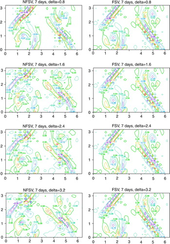
Fig. 10.  The prediction errors caused by the NFSVs and the FSVs in the QG model (denoted by NFSV-n and FSV-n) and those caused by the FSVs in the linearised QG model (denoted by FSV-l). The horizontal axis represents the perturbation magnitudes, and the vertical axis describes the prediction errors in terms of the energy. (a) uses an optimisation time of 2 d, and (b) uses an optimisation time of 7 d.

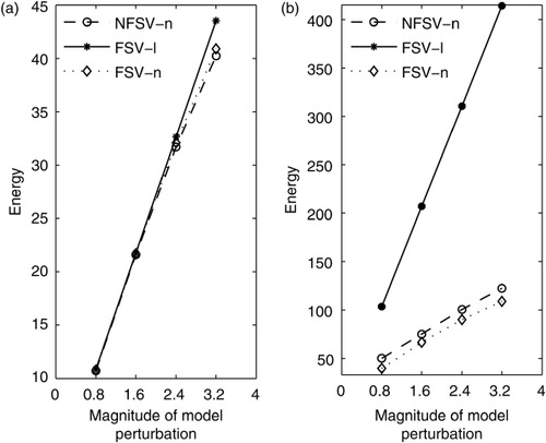
Fig. 11.  Patterns of the stream functions of the prediction errors caused by (a) the FSV in the linearised QG model, (b) the FSV in the non-linear QG model, and (c) the NFSV in the non-linear QG model, where the optimisation is 7 d and the model perturbation magnitude is 1.6 in terms of the chosen norm.

Fig. 12.  The meridional-mean of the stream function of prediction errors (left column) and the corresponding meridional wind (right column) caused by (a, b) the FSV in the linearised QG model, (c, d) the FSV in the non-linear QG model, and (e, f) the NFSV in the non-linear QG model. The optimisation time is 7 d, and the model perturbation magnitude is 1.6.

Fig. 13.  The patterns of the stream function of the prediction error caused by the optimal forcing in the linearised QG model (left column) and the differences between the perturbation stream function induced by the optimal forcing in the non-linear QG model and in the linearised QG model (right column). The latter indicates the non-linear effects of perturbation advection on the perturbation growth. (a) and (b) are for the FSV, and (c) and (d) are for the NFSV. Both the FSV and NFSV are computed with an optimisation time of 7 d and a model perturbation magnitude of 1.6.

5. Summary and discussion

In this article, we extend the FSV approach to the non-linear field and propose the concept of a NFSV. The advantage of the NFSV approach is that it sufficiently considers the effects of non-linearity. The NFSVs can determine the time-dependent tendency error of a model. In this article, because the FSV is constant in time and the goal is to compare FSV and NFSV, we only study the constant NFSV, which may describe a type of model systematic error that causes significantly large prediction errors at the prediction time. A two-dimensional QG model is adopted to study the NFSV model errors. Two non-linearly stable states (denoted by Ref-1 and Ref-2) of the QG model are chosen as reference states (or basic flows) to describe the results. Furthermore, the Ref-1 basic flow is zonal and includes regions of strong velocity shear, whereas the Ref-2 basic flow is approximately meridional with two deformation fields containing strong velocity shears. After computing the NFSVs and the corresponding linear FSVs, our results show that the NFSVs have a phase in which the perturbation stream function tends to be contracted around the strong velocity shear region and tilted against the basic shear, presenting an asymmetric structure, especially for large tendency perturbations. Due to the absence of non-linearity, the FSVs for the Ref-1 tend to be more symmetric and cover a larger region than the NFSVs; in contrast, the FSVs for the Ref-2 only cover a slightly larger region compared to the NFSVs. NFSVs and FSVs also cause different prediction errors. For the Ref-1 basic flow, the magnitudes of the prediction errors caused by the FSVs in the non-linear QG model are significantly smaller than those caused by the FSVs in the linearised QG model for large tendency perturbations and/or long optimisation times. Non-linearities in the QG model then have a damping effect on the linear evolution of the tendency perturbations. Furthermore, we demonstrate that the prediction errors caused by the NFSVs in the non-linear QG model are obviously larger than those caused by the FSVs; therefore, the NFSVs are more applicable than the FSVs in numerically describing the optimal tendency perturbations. Physically, the constant tendency errors of the NFSV structure tend to reduce the non-linear damping effect and have the most potential for extracting energy from the basic flows and exhibiting optimal growth. For the Ref-2 basic flow, the non-linearity still suppresses the growth of the perturbation. Nevertheless, the NFSVs only slightly reduce this damping effect of the non-linearity. In this case, the evolutions of the prediction errors caused by the NFSVs and FSVs tend to have nearly the same amplitudes. It is therefore clear that the differences between the NFSVs and FSVs depend not only on the tendency perturbation magnitudes and/or optimisation times but also on the properties of the basic flows. Although we demonstrate that the Ref-2 NFSVs can be approximated by the corresponding FSVs, it is difficult for us to validate this argument in advance. Therefore, for a non-linear system, we would use the NFSVs rather than the FSVs to study the predictability of weather and climate. In particular, the differences between the NFSVs and FSVs for the Ref-1 basic flow show the usefulness of the NFSVs in revealing the effects of non-linearity on the predictability. The NFSV may therefore be a useful non-linear technique for exploring the predictability problems introduced by model errors.

In this study, we regard the constant tendency perturbations as constant tendency errors and compute the NFSVs, which may describe the model systematic errors that cause progressively large prediction errors at a prediction time. In this case, the patterns of the NFSVs may allow us to find the regions in which the predictions are most sensitive to model systematic errors; therefore, the corresponding physical processes should be better described by the models. For example, we demonstrate in this article that the NFSVs have a phase in which the perturbation stream function tends to be contracted around the region of strong velocity shear; thus, the predictions generated by the two-dimensional QG model may be highly sensitive to the systematic errors of the model in the strong velocity shear region and the physical processes associated with this region should be better described by the models. In numerical predictions, we can determine an optimal external forcing to offset the model uncertainties by assimilating observations in this sensitive region. In addition, if we take the constant tendency perturbation as an external forcing with a particular physical meaning, the NFSVs may describe the external forcings to which the weather and climate are significantly sensitive. Furthermore, if the NFSVs are superimposed on an external forcing with a particular physical meaning, they can be used to investigate the effects of the external forcing uncertainties on the prediction results. Of course, these theories should be realised by applying them to physical problems of interest. It is anticipated that the NFSV approach may play an important role in addressing the second type of predictability problem.

Riviere et al. (2008) demonstrated that the non-linear singular vectors (non-linear optimal initial perturbations) of a two-layer QG model tend to have larger meridional extensions than the singular vectors (linear optimal initial perturbations). However, we demonstrated in this article that the FSVs tend to have larger extensions than the NFSVs. It is clear that differences may exist in the effects of non-linearity on the tendency perturbations and initial perturbations. Despite the fact that the NFSVs provide useful information about the model systematic errors, as demonstrated above, it is unclear why the effects of non-linearity on the model perturbations and initial perturbations are different. It may be challenging to address this question, which requires further investigation.

In numerical experiments, we examine the norms such as the L ₂ norm, the potential enstrophy norm and the energy norm in measuring the magnitudes of the constant tendency perturbations and/or the prediction errors caused by them. However, in some cases, the algorithm adopted here may not capture the maximum of the cost function associated with the NFSVs and allow the resultant NFSVs to comprise many small scales; alternatively, the resultant NFSVs do not possess clear physical meanings. In this article, after several attempts, we finally chose the L ₂ norm to measure the tendency perturbation magnitudes and the energy norm to measure the evolution of the prediction error caused by constant tendency errors and reveal the effects of non-linearity on the NFSV structures. Furthermore, we are almost able to provide a physical explanation for the structure of the NFSVs and why the NFSVs cause a larger perturbation growth than the FSVs. Therefore, the norm adopted in this study may be physically relevant.

To study the effects of the model parameter errors on predictability, Mu et al. (2010) proposed the CNOP-P approach to solve the optimal model parameter perturbation. Although the NFSV used to describe the model systematic errors can be derived using the CNOP-P approach, the constant tendency perturbation requires a different reasoning than that applied to a specific model parameter perturbation. In fact, the perturbation superimposed on a model parameter represents a parameter error, whereas the constant tendency perturbation may describe the combined systematic errors of physical processes that are not explicitly or not entirely correctly described by the model equations. Furthermore, the NFSVs allow us to investigate the spatial structures of the model systematic errors. Additionally, the NFSVs can be generalised to be time-dependent and can then describe much realistic model errors. Therefore, the NFSVs are much more general than the optimal parameter perturbations associated with the CNOP-P approach.

Predictability studies are challenging due to the non-linearity and complexity of atmospheric and oceanic motions. In particular, the predictability problems associated with model errors pose great difficulties due to the lack of effective approaches. In this article, we propose the NFSV approach to address certain model errors. It is expected that this approach will play an important role in studying the predictability problems associated with model errors and provide ideas for improving weather and climate predictabilities.

6. Acknowledgements

The authors are very grateful for useful comments provided by the two reviewers. This work was jointly sponsored by the Knowledge Innovation Program of the Chinese Academy of Sciences (No. KZCX2-YW-QN203), the National Basic Research Program of China (No. 2010CB950400 and 2012CB955202), and the National Natural Science Foundation of China (No. 41176013).

7. Appendix

The first-order variational of J ₁(f)

A1

With integration by parts, we can obtain

and

Then, we derive δJ ₁ as follows:A2

where denotes an adjoint operator. Then, we obtainA3

References

- Arakawa A. Computation design for long-term numerical integrations for the equations of atmospheric motions. J. Comput. Phys. 1966; 1: 119–143. 10.3402/tellusa.v65i0.18452.
- Barkmeijer J. Constructing fast-growing perturbations for the nonlinear regime. Q. J. Roy. Meteor. Soc. 1996; 53: 2838–2851.
- Barkmeijer J. Iversen T. Palmer T. N. Forcing singular vector and other sensitivity model structures. J. Optim. 2003; 129: 2401–2423. 10.3402/tellusa.v65i0.18452.
- Birgin E. G. Martinez J. M. Raydan M. Nonmonotone spectral projected gradient methods on convex sets, SIAM. Q. J. Roy. Meteor. Soc. 2000; 10: 1196–1211.
- Buizza R. Miller M. Palmer T. N. Stochastic representation of model uncertainties in the ECMWF ensemble prediction system. 1999; 125: 2887–2908. 10.3402/tellusa.v65i0.18452.
- Cai M. Kalnay E. Toth Z. Bred vectors of the Zebiak-Cane model and their potential application to ENSO predictions. J. Clim. 2003; 16: 40–55.
- D'Andrea F. Vautard R. Reducing systematic errors by empirically correcting model errors. Tellus. 2000; 52A: 21–41.
- Duan, W. S, Liu, X. C, Zhu, K. Y and Mu, M. 2009. Exploring the initial errors that cause a significant “spring predictability barrier” for El Nino events. J. Geophys. Res. 114, C04022. 10.3402/tellusa.v65i0.18452.
- Duan, W. S and Mu, M. 2006. Investigating decadal variability of El Nino-Southern Oscillation asymmetry by conditional nonlinear optimal perturbation. J. Geophys. Res. 111, C07015. 10.3402/tellusa.v65i0.18452.
- Duan W. S. Mu M. Wang B. Conditional nonlinear optimal perturbation as the optimal precursors for El Nino-Southern Oscillation events. J. Geophys. Res. 2004; 109: D23105.10.3402/tellusa.v65i0.18452.
- Duan, W. S, Xu, H.and Mu, M. 2008. Decisive role of nonlinear temperature advection in El Nino and La Nina amplitude asymmetry. J. Geophys. Res. 113, C01014. 10.3402/tellusa.v65i0.18452.
- Dudhia J. A nonhydrostatic version of the Penn State-NCAR mesoscale model: validation tests and simulation of an Atlantic cyclone and cold front. Mon. Wea. Rev. 1993; 121: 1493–1513.
- Farrell B. Optimal excitation of baroclinic waves. J. Atmos. Sci. 1989; 46: 1193–1206.
- Farrell B. Ioannou P. J. Distributed forcing of forecast and assimilation systems. J. Atmos. Sci. 2005; 62: 460–475. 10.3402/tellusa.v65i0.18452.
- Gutowski W. J.Jr. Baroclinic adjustment and midlatitude temperature profiles. J. Atmos. Sci. 1985; 42: 1733–1745.
- Hamill T. M. Snyder C. Morss R. E. A comparison of probabilistic forecasts from bred, singular-vector, and perturbed observation ensembles. Mon. Wea. Rev. 2000; 128: 1835–1851.
- Houtekamer P. L. Derome J. Methods for ensemble prediction. Mon. Wea. Rev. 1995; 123: 2181–2196.
- Houtekamer P. L. Lefaivre L. Derome J. Ritchie H. Mitchell H. L. A system simulation approach to ensemble prediction. Mon. Wea. Rev. 1996; 124: 1225–1242.
- Jiang Z. N. Mu M. A comparisons study of the methods of conditional nonlinear optimal perturbations and singular vectors in ensemble prediction. Adv. Atmos. Sci. 2009; 26(3): 465–470. 10.3402/tellusa.v65i0.18452.
- Lacarra J. Talagrand O. Short-range evolution of small perturbations in a barotropic model. Tellus. 1988; 40A: 81–95. 10.3402/tellusa.v65i0.18452.
- Le Dimet F. X. Talagrand O. Variational algorithms for analysis and assimilation of meteorological observations: theoretical aspects. Tellus. 1986; 38A: 97–110. 10.3402/tellusa.v65i0.18452.
- Liu D. C. Nocedal J. On the limited memory method for large scale optimization. Math. Program. B. 1989; 45(3): 503–528. 10.3402/tellusa.v65i0.18452.
- Lorenz E. A study of the predictability of a 28-variable atmospheric model. Tellus. 1965; 17: 321–333. 10.3402/tellusa.v65i0.18452.
- Lorenz E. N. Climate Predictability: The Physical Basis of Climate Modelling. Global Atmospheric Research Programme Publication Series, No. 16, World Meteorology Organization, Geneva.1975; 132–136.
- Mak M. Cai M. Local barotropic instability. J. Atmos. Sci. 1989; 46: 3289–3311.
- Moore A. M. Kleeman R. The dynamics of error growth and predictability in a coupled model of ENSO. Q. J. Roy. Meteor. Soc. 1996; 122: 1405–1446. 10.3402/tellusa.v65i0.18452.
- Moore A. M. Kleeman R. Stochastic forcing of ENSO by the intraseasonal oscillation. J. Clim. 1999; 12: 1199–1220.
- Mu M. Duan W. S. Wang B. Conditional nonlinear optimal perturbation and its applications. 2003; 10: 493–501. 10.3402/tellusa.v65i0.18452.
- Mu, M, Duan, W. S and Wang, B. 2007a. Season-dependent dynamics of nonlinear optimal error growth and El Nino-Southern Oscillation predictability in a theoretical model. Nonlin. Process. Geophys. 112, D10113. 10.3402/tellusa.v65i0.18452.
- Mu M. Duan W. Wang Q. Zhang R. An extention of conditional nonlinear optimal perturbation approach and its applications. J. Geophys. Res. 2010; 17: 211–220. 10.3402/tellusa.v65i0.18452.
- Mu M. Shepherd T. G. Nonlinear stability of multilayer quasi-geostrophic flow. Nonlin. Process. Geophys. 1994; 75: 21–37. 10.3402/tellusa.v65i0.18452.
- Mu M. Sun L. Dijkstra H. The sensitivity and stability of the ocean's thermocline circulation to finite amplitude freshwater perturbations. 2004; 34: 2305–2315.
- Mu, M, Xu, H and Duan, W. 2007b. A kind of initial errors related to “spring predictability barrier” for El Nino events in Zebiak-Cane model. Geophys. Astrophys. Fluid. Dyn. 34, L03709. 10.3402/tellusa.v65i0.18452.
- Mu M. Zeng Q. C. New development on existence and uniqueness of solutions to some models in atmospheric dynamics. J. Phys. Oceanogr. 1991; 8: 383–398. 10.3402/tellusa.v65i0.18452.
- Mu M. Zhou F. Wang H. A method for identifying the sensitive areas in targeted observations for tropical cyclone prediction: conditional nonlinear optimal perturbation. Geophys. Res. Lett. 2009; 137(5): 1623–1639. 10.3402/tellusa.v65i0.18452.
- Mylne K. R. Evans R. E. Clark R. T. Multi-model multi-analysis ensembles in quasi-operational medium-range forecasting. Adv. Atmos. Sci. 2002; 128: 361–384. 10.3402/tellusa.v65i0.18452.
- Nakamura N. Baroclinic–barotropic adjustments in a meridionally wide domain. 1999; 56: 2246–2260.
- Oortwijn J. Barkmeijer J. Perturbations that optimally trigger weather regimes. Mon. Wea. Rev. 1995; 52: 3932–3944.
- Palmer, T. N, Molteni, F, Mureau, R, Buizza, R, Chapelet, P. and co-authors. 1992. Ensemble prediction. ECMWF Research Department Tech. Memo. 188, ECMWF, Shinfield Park, Reading, England. 45. pp.
- Pedlosky J. Geophysical Fluid Dynamics. Springer-Verlag, New York.1979
- Powell M. J. D. VMCWD: A FORTRAN Subroutine for Constrained Optimization. DAMTP Report 1982/NA4, University of Cambridge, England.1982
- Riviere O. Lapeyre G. Talagrand O. Nonlinear generalization of singular vectors: behavior in a baroclinic unstable flow. 2008; 65: 1896–1911. 10.3402/tellusa.v65i0.18452.
- Riviere O. Lapeyre G. Talagrand O. A novel technique for nonlinear sensitivity analysis: application to moist predictability. 2009; 135: 1520–1537. 10.3402/tellusa.v65i0.18452.
- Roads J. O. Predictability in the extended range. 1987; 44: 1228–1251.
- Samelson R. G. Tziperman E. Instability of the chaotic ENSO: the growth-phase predictability barrier. J. Atmos. Sci. 2001; 58: 3613–3625.
- Shutyaev V. Le Dimet V. F.-X. Gejadze I. On optimal solution error covariances in variational data assimilation. Q. J. Roy. Meteor. Soc. 2008; 23: 185–206. 10.3402/tellusa.v65i0.18452.
- Simmons A. Hollingsworth A. Some aspects of the improvement in skill of numerical weather prediction. J. Atmos. Sci. 2002; 128: 647–677. 10.3402/tellusa.v65i0.18452.
- Tanguay M. Bartello P. Gauthier P. Four dimensional data assimilation with a wide range of scales. J. Atmos. Sci. 1995; 47A: 974–997.
- Tennekes H. Karl Popper and the Accountability of Numerical Forecasting. In New Developments in Predictability. ECMWF Workshop Proceedings, ECMWF, Shinfield Park, Reading, UK.1991
- Terwisscha A. D. Dijkstra H. Conditional nonlinear optimal perturbations of the double-gyre ocean circulation. Tellus. 2008; 15: 727–734. 10.3402/tellusa.v65i0.18452.
- Thompson C. J. Initial conditions for optimal growth in a coupled ocean-atmosphere model of ENSO. 1998; 55: 537–557.
- Thompson P. Uncertainty of the initial state as a factor in the predictability of large scale atmospheric flow patterns. Nonlin. Process. Geophys. 1957; 9: 275–295. 10.3402/tellusa.v65i0.18452.
- Toth Z. Kalnay E. Ensemble forecasting at NCEP and the breeding method. J. Atmos. Sci. 1997; 127: 3297–3318.
- Tung K. K. Barotropic instability of zonal flows. Tellus. 1981; 38: 308–321.
- Wu X. G. Mu M. Impact of horizontal diffusion on the nonlinear stability of thermohaline circulation in a modified box model. Mon. Wea. Rev. 2009; 39: 798–805. 10.3402/tellusa.v65i0.18452.
- Xue Y. Cane M. A. Zebaik S. E. Predictability of a coupled model of ENSO using singular vector analysis. Part I: optimal growth in seasonal background and ENSO cycles. J. Atmos. Sci. 1997; 125: 2043–2056.
- Zebiak S. E. Cane A. A model El Nino-Southern Oscillation. J. Phys. Oceanogr. 1987; 115: 2262–2278.
7. Appendix
The first-order variational of J 1(f)