The linearisation of maps in data assimilation

Abstract

For the purpose of linearising maps in data assimilation, the tangent-linear approximation is often used. We compare this with the use of the ‘best linear’ approximation, which is the linear map that minimises the mean square error. As a benchmark, we use minimum variance filters and smoothers which are non-linear generalisations of Kalman filters and smoothers. We show that use of the best linear approximation leads to a filter whose prior has first moment unapproximated compared with the benchmark, and second moment whose departure from the benchmark is bounded independently of the derivative of the map, with similar results for smoothers. This is particularly advantageous where the maps in question are strongly non-linear on the scale of the increments. Furthermore, the best linear approximation works equally well for maps which are non-differentiable. We illustrate the results with examples using low-dimensional chaotic maps.

• tangent-linear approximation
• incremental 4D-Var
• extended Kalman smoother

1. Introduction

The methods currently used for large-scale data assimilation in the earth sciences can be viewed as approximate implementations of the Kalman filter or Kalman smoother, and their variational equivalents. These are only optimal for linear forecast and observation operators, while the forecast maps encountered in the earth sciences are non-linear.

One important class of methodologies, including the extended Kalman filter and smoother and incremental four-dimensional variational assimilation (4D-Var), attempts to get round this by linearisation. In practice, this has nearly always meant approximating each map f(x+ δ ) by its first-order Taylor polynomial f(x)+f′(x) δ , the so-called ‘tangent-linear’ (TL) approximation. If the distribution of the perturbations δ is known, we may form instead the ‘best linear’ (BL) approximation , in which , are chosen to minimise the mean square error in this approximation. We will designate these approximations the TLA and BLA, respectively. In this article we consider the merits of the BLA in data assimilation.

We begin in Section 2 by giving some of the properties of the BLA. Versions of the same idea have been considered by others, such as by Gelb (1974) who call it ‘statistical linearisation’, and by Lorenc and Payne (2007) where it is termed ‘optimal regularisation’. The reason for this latter terminology will be apparent in Section 3, where we explore the properties of the BLA through one application, the regularisation of a parametrisation of grid-box cloud fraction.

The main focus in this article is on the use of the BLA in the data assimilation-forecast cycle where the non-linearity is in the forecast map. The case where the observation operators are also non-linear is considered briefly in an appendix.

For optimal filtering, to form the prior pdf at the next time level the posterior pdf from the former time level is evolved forward in time by the Chapman–Kolmogorov equation [e.g. Jaswinski (1970)]. If the forecast map is linear and the posterior pdf is Gaussian, this is exactly accomplished by the predictive part of the Kalman filter. For non-linear maps, we should use the Chapman–Kolmogorov equation in its full form, but a popular approach in practice is to apply the Kalman filter to a linearised map, giving rise to the extended Kalman filter (EKF). Similarly, for the Kalman smoother (and its variational equivalent, 4D-Var) which is the optimal smoother for linear maps and Gaussian pdfs, a common approach is to linearise the non-linear map to form the (generally suboptimal) extended Kalman smoother (EKS) and incremental 4D-Var.

Normally for the EKF, EKS and incremental 4D-Var the TLA is used. In Lorenc (1997), the limitations of the TLA for 4D-Var were recognised and Lorenc coined the term ‘perturbation forecast’ (PF) model to describe a linear model appropriate for the evolution of finite perturbations. Errico and Raeder (1999) also recognised that it is the accuracy of the linear model in evolving finite amplitude perturbations which is important for applications, and assessed how well the tangent-linear to some meteorological models performed in this regard. Lawless et al. (2005) considered specifically the non-tangent-linear model arising from discretising a linearisation of the continuous non-linear equations (rather than linearising a discretisation, as in a TL model), from the point of view of showing that the use of such a model would not necessarily degrade the assimilation compared with a TL model.

It has long been accepted when linearising components of non-linear models for adjoint applications such as incremental 4D-Var, that physical parametrisations in particular may need to be ‘regularised’ rather than the TL taken directly. Lorenc and Payne (2007) used the BLA to construct an optimal regularisation, and suggested applying the principle to the whole model rather than merely individual components. The present work follows this up analytically, and thereby provides a justification for the ‘PF not TL’ philosophy in cycled data assimilation.

In order to develop and compare TLA and BLA based EKFs, we begin in Section 4 by using the same approach we used to find the BLA to maps to derive a generalisation of the Kalman filter for non-linear propagating maps. Specifically, we find the analysis linear in the observations which minimises mean square analysis error. This is equivalent (see Appendix A.1) to specialising the optimal filter obtained from Bayes’ rule and the Chapman–Kolmogorov equation by approximating where necessary each pdf by a Gaussian one with the same first two moments. The resulting prediction step has been used before as the basis for non-linear generalisations of the Kalman filter, such as the ‘unscented Kalman filter’ of Julier and Uhlmann (1997).

In Section 5 the non-linear filter of Section 4 is approximated by the TL and BL approximations to form TLA and BLA based EKFs. We show that the latter can be expected to outperform the former. In Section 6, we illustrate the methods and the results by comparing the TLA and BLA in filters assimilating noisy observations of states of the Duffing map, a chaotic non-linear map which discretises the Duffing oscillator.

In Sections 7–9 we treat smoothers in an analogous way to the treatment of filters in Sections 4–6. In Section 7, we develop a generalisation of the Kalman Smoother for non-linear propagating maps, and use it in Section 8 to develop TLA and BLA based EKSs. These are of particular interest as they are equivalent to TLA and BLA based versions of incremental 4D-Var. Again we show the latter can be expected can be expected to outperform the former, and give examples in Section 9.

2. Best linear approximation

We begin by formulating and obtaining the best linear approximation, and comparing with the tangent-linear approximation. Suppose we have a function f for which we seek a local linear approximationwhere is a vector and a matrix. If f is C ¹, we might choose , , so the local linear approximation to f(x+ δ ) is the first-order Taylor polynomial f(x)+f′(x) δ . This is the tangent-linear approximation or TLA, usually encountered in the adjoint applications literature in the form f(x+ δ )−f(x)≈f′(x) δ .

However, if we know the pdf of δ we may seek the ‘best local linear approximation’ in the sense of minimising1 over and for a given symmetric positive-definite matrix A. This is termed ‘statistical linearisation’ in Gelb (1974) and, for reasons discussed in Section 3 below, ‘optimal regularisation’ in Lorenc and Payne (2007).

If is minimised by and , then differentiating with respect to and and setting the derivatives to zero we obtain respectively the vector and matrix equations:2 Solving the simultaneous equations [eq. (2)] we see that f ⁽⁰⁾(x) and f ⁽¹⁾(x) are independent of A and given by3 4 So the linear approximation to f(x+ δ ) which minimises mean square linearisation error, and which we call the best linear approximation or BLA, is f ⁽⁰⁾(x)+f ⁽¹⁾(x) δ . Noting that if this approximation is used then linearisation error itself is5 it follows that eq. (2) may be written6 The coefficients f ⁽⁰⁾(x) and f ⁽¹⁾(x) in the BLA share with the coefficients in the TLA the property of being linear as a function of f, i.e. if h=α f+β g then for j=0,1which can be useful for constructing BLAs.

Some obvious but important points of difference or comparison between the BLA and TLA are:

(a) Whereas the coefficients of the TLA are a function only of f, those of the BLA are a function of f and the pdf of the increments.

(b) In forming the BLA, unlike the TLA, f does not need to be differentiable. The BLA captures the local form of f on the scale of the perturbations δ , rather than the instantaneous derivative. This can be an important distinction where f contains more than one scale or contains sudden changes in derivative, as for example is often the case with physical parametrisations.

(c) In the limit that the perturbations become small compared with the scale of the non-linearity, for example if f is C ¹ and the distribution of δ tends to a Dirac delta function, then f ⁽⁰⁾(x)→f(x) and f ⁽¹⁾(x)→f′(x). Thus the TLA is appropriate for infinitesimal perturbations.

These points are illustrated by the example which follows.

3. Example of best linear approximation: regularisation of grid-box cloud fraction

As an example, consider the parametrisation of grid-box cloud fraction Φ as a function of total water q _t , liquid temperature T _L and pressure p given in Smith (1990):7 where8 where q _sat is the saturation specific humidity and RH _c is a constant. Suppose we require a linear approximation9 to this function, e.g. for use in the linear model in incremental 4D-Var. Note that if Q _N ≤−1 or Q _N ≥1 then dΦ/dQ _N =0, so the TLA Φ(Q _N +δQ _N )≈Φ(Q _N )+Φ′(Q _N )δQ _N will simply return Φ(Q _N ) for Q _N in that range. Traditionally such functions have been ‘regularised’, i.e. replaced by slightly smoothed versions whose first-order Taylor polynomial better approximates the non-linear function. In this case, a regularisation which has been used is to replace Φ by Φ_reg 10 Clearly this regularisation is ad hoc; there are any number of other smooth functions which could have been chosen to approximate Φ. However, if we know the distribution of δQ _N then we see the BLA of Section 2 constitutes an ‘optimal’ regularisation, in the sense of minimising mean square linearisation error.

In the 4D-Var context δQ _N are, at convergence of the 4D-Var minimisation, analysis increments, and we can accumulate statistics on them from past analyses. The simplest way to then form Φ⁽⁰⁾ and Φ⁽¹⁾ is by discretising eqs. (3) and (4) directly (i.e. replace the integrals defining the expectations by finite summations using the empirical data). However, to illustrate some features of the BLA we will approximate the empirical distribution by an analytic one. The generalised normal distribution is a family of distributions which for a one-dimensional independent variable x with mean x ₀ have pdf11 where p, σ are parameters. In the Gaussian or standard normal distribution, p=2. We find empirically that δQ _N is approximately distributed with a generalised normal distribution with p=1, zero mean and σ≈0.4, independently of Q _N .

We consider four linearisations [eq. (9)] of the cloud function [eq. (7)] about Q _N , which will be denoted (i)–(iv). For (i), we use the TLA, so Φ₀(Q _N )=Φ(Q _N ) and Φ₁(Q _N )=Φ′(Q _N ). For (ii)–(iv), we use the BLA of Φ(Q _N ) calculated for δQ _N distributed with a range of pdfs. In detail, we will in each case compute the BLA for δQ _N distributed with a generalised normal distribution [eq. (11)] with p=1, and for (ii) σ=0.8, for (iii) σ=0.4 (the correct value), and for (iv) σ=0.1. Fig. 1 shows

Fig. 1 (a) pdf of generalised normal distribution (11) with p=1 for σ=0.8 (blue), σ=0.4 (green) and σ=0.1 (red); (b) cloud fraction Φ (black) and Φ⁽⁰⁾ for various σ as in (a); (c) Φ′ (black) and Φ⁽¹⁾ for various σ as in (a); (d) linearisation error assuming true pdf has σ=0.4, using the TLA (black) and the BLA with various σ as in (a).

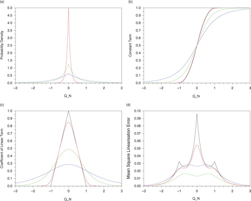
(a) The generalised normal distribution with p=1 for σ=0.8 (blue), σ=0.4 (green) and σ=0.1 (red);

(b) The constant term Φ₀(Q _N ) in eq. (9) computed according to the methods described above. The black curve uses the TLA as in (i), so is simply Φ(Q _N ). The other curves use the BLA with σ=0.8 (blue), σ=0.4 (green), σ=0.1 (red).

(c) The coefficient Φ₁(Q _N ) in eq. (9) computed according to the methods described above, same colour scheme as (b).

(d) For the last plot we suppose δQ _N has a generalised normal distribution [eq. (11)] with p=1 and σ=0.4, and compute the mean square linearisation error using the linearisations (i)–(iv). Note that in this scalar case mean square linearisation error is the function of eq. (1) with A=1.

3.1. Remarks

 (1) As noted above, as σ→0 we see [Fig. 1b] that Φ⁽⁰⁾ converges to Φ and [Fig. 1c] that Φ⁽¹⁾ converges to Φ^′.

 (2) With conventional regularisation Φ is approximated by smooth Φ _reg and one would use Φ₀(Q _N )=Φ _reg and Φ₁(Q _N )=Φ _reg ′, so Φ₁(Q _N )=Φ₀′(Q _N ). However for the BLA, in general Φ⁽¹⁾ is not the derivative of Φ⁽⁰⁾.

 (3) Φ⁽⁰⁾ is formed by taking a weighted average of nearby values of Φ, and as σ increases greater distances are given greater weights, so for fixed Q _N we have as σ→∞ [Fig. 1b]. Similarly, for fixed Q _N we have Φ⁽¹⁾(Q _N )→0 as σ→∞ [Fig. 1c].

 (4) The mean square linearisation error using the BLA and the correct pdf (green curve in Fig. 1d) is always less and mostly a small fraction of that using the TLA [black curve in Fig. 1d]. The regularisation is typical in that it smooths Φ but is everywhere close to Φ in the C ⁰ norm, and actually affords very little benefit compared with the TLA – its linearisation error is nearly as large as that of the tangent linear.

4. A non-linear generalisation of the Kalman Filter

The main purpose of this article is to examine and improve the use of linearised maps in data assimilation. To do this we need a non-linear generalisation of the predictive step of the Kalman filter, which we can approximate using the TLA and BLA, and then use as a benchmark against which to compare the impact of the two approximations.

The generalisation we use is obtained by applying the BLA approach to the state estimation problem in the forecast-assimilation cycle. This is equivalent to the familiar linear minimum variance estimator of, for example, Sage and Melsa (1971: Section 6.6). To keep the article self-contained and highlight the connection with the BLA we derive this filter in the same way as we did the BLA. The resulting generalisation of the prediction stage of the Kalman filter [eq. (20) below] has been used previously, for filtering polynomial systems in Luca et al. (2006), and notably in Julier and Uhlmann (1997) as the basis for the unscented Kalman filter.

Suppose we have states x _i , noisy observations y _i of these states and a noisy model f _i which evolves the state from time level i to i+1. Denote our best estimate or analysis of x _i given observations y ₁,..,y _i by . We suppose we have an analysis at time i, and we seek to use an observation at time i+1 to form an analysis at i+1. In summary, we have12 where ε _i , w _i , v _i+1 are random variables, the pdfs of which are supposed known. At this stage we do not require these pdfs to be Gaussian, though for simplicity we shall suppose that ε _i , w _i , v _i+1 have zero mean and are uncorrelated with each other and with all other quantities, though weaker hypotheses are possible. The covariance of the analysis error ε _i is denoted P _i∣i .

In the same spirit as the BLA for maps we may seek the best linear analysis , that is, we seek K _i+1, c _i+1 depending on and the pdfs of ε _i , w _i , v _i+1 such that if is of the form13 then14 is minimised, where the expectation is over ε _i , w _i , v _i+1. As before, the solution is independent of A. Set15 Setting the derivatives of eq. (14) with respect to c _i+1, K _i+1 to zero, solving the resulting simultaneous equations and using eq. (12) to express all expectations in terms of ε _i , w _i , v _i+1, we obtain after some manipulation16 17 where18 the expectations in eq. (18) being over ε _i . The notation is consistent with standard filtering theory (see Appendix A.1).

None of this requires Gaussianity of ε _i , w _i , v _i+1. However, while the pdfs of w _i , v _i+1 are externally given, the pdf of ε _i (which we need to compute the expectations) is the analysis error from the previous time level. By direct calculation, we find the covariance of to be19 To close the system we will approximate the pdf of ε _i+1 as a Gaussian with zero mean and covariance [eq. (19)], and use this as the pdf at the next time level.

Putting this all together we obtain what we will term the minimum variance filter given by eqs. (20) and (21) below, which generalises the Kalman filter in the case where the propagating map f _i is non-linear. The notation ε _i ~N(0, P _i∣i ) signifies that ε _i is normally distributed with zero mean and covariance P _i∣i . We show in Appendix A.1 how for Gaussian v _i+1 and w _i we obtain the same algorithm from Bayes’ rule and the Chapman–Kolmogorov equation if we approximate the prior pdf by a Gaussian with the same first two moments.

For i=0,1,…

Predict20 where ε _i ~N(0, P _i∣i )

Update:21

Because our observation operator is linear (in fact, here the identity) the update step eq. (21) is unchanged from the standard Kalman filter. As noted above, the predict stage eq. (20) has been used before as the basis for non-linear generalisations of the Kalman filter, such as in Julier and Uhlmann (1997) as the basis for the unscented Kalman filter.

If f _i is linear then eq. (20) simplifies to the usual Kalman filter, and if f _i is non-linear and we replace it by its TL approximation we obtain the usual form of the EKF, a point expanded upon in Section 5 below.

Readers familiar with ensemble filters may be interested in the relationship between the minimum variance filter, eqs. (20) and (21), and an ensemble Kalman Filter (EnKF) with infinite ensemble size. Assuming the EnKF is cycled in the usual way it differs in the following respect. We may choose the perturbed analyses used in the initial cycle of the EnKF to be distributed as , but on cycles after the first the perturbed analyses in the EnKF will only have a Gaussian distribution if the forecast map is linear. This distinguishes it from the minimum variance filter [eq. (20)] which always uses Gaussian analysis errors. The two filters would coincide (in the limit of an infinite ensemble size for the EnKF) if the EnKF was modified so that on every cycle its analysis ensemble was formed as a random sample drawn from a Gaussian distribution with covariance equal to the usual EnKF analysis covariance.

5. Linearisation stratagems for the prediction part of the update-prediction cycle

For small systems one might be able to compute the covariance in eq. (20) exactly, and for large systems it could be approximated by a small ensemble. In the standard form of the EKF, is replaced [in both parts of eq. (20)] by its TL approximation. Here we shall compare this approximation with the BL approximation. By examining the impact of these approximations on eq. (20), we can compare the impact of making the TLA and BLA on the quality of the data assimilation system.

If f _i is C ¹ and we apply Taylor's theorem to expand it about the analysis , we have22 where is the error in the TL approximation. Substituting eq. (22) into eq. (20), we get23 where is the error in P _i+1∣i arising through the use of the TLA:24 where .

If we make an expansion based on the BLA of f _i about the analysis 25 where is the error in the BL approximation, and substitute eq. (25) into eq. (20), we get26 From eq. (6) we know that , so does not appear in eq. (26). The term representing the error in P _i+1∣i if the BLA is made has some very interesting properties. We have27 but by virtue of eq. (6) and the fact ε _i has zero mean28 so29

In the light of the foregoing several key observations may be made:

(a) While in eq. (24) is merely an error, and may be positive-definite, negative-definite or indefinite, is a covariance; specifically, it is the covariance of linearisation error.

(b) As such is positive semi-definite. Therefore if it is entirely neglected and for the prior covariance P _i+1∣i we use then we always underestimate the true prior covariance.

(c) As noted above, if the BLA is used there is no approximation in the prior [first line of eq. (26)] compared with the minimum variance filter of Section 4.

In view of its formulation we also expect the BLA to lead to an improved prior covariance P _i+1∣i than the TLA, particularly when on the scale of the increments f _i is strongly non-linear. Specifically we have the following:

(d) While in eq. (24) is a function of the pointwise derivative of f _i at , which may be very large and erratic, is bounded independently of as follows. is positive semi-definite, so all its eigenvalues are non-negative, but the sum of its eigenvalues equals the trace of . Using the definitions of BLA and ℓℓ ^BL _i , and the fact that for any matrices A, B trace(AB)=trace(BA), we have30 where the expectation is over ε _i . Thus, the eigenvalues of are all non-negative, but their sum is bounded by the minimum possible mean square linearisation error.

5.1. Filters using the TLA and BLA

At one extreme, if we compute the linearisation error matrices and exactly as defined by eqs. (24) and (29) we reproduce the minimum variance filter of Section 4 above. At the other extreme, if we set them to zero we obtain in the TLA case the standard EKF. However, as noted in Fisher et al. (2005), in this case analysis errors are very large. Even though they were working in a perfect model environment with Q _i =0, they included a diagonal Q _i to allow for linearisation error, see especially their Fig. 1. Effectively they relabelled as Q _i and then parametrised it by one scalar.

We will follow a similar strategy and allow for simple parametrisations of and . Fisher et al. (2005) showed this was important in the TL case; we anticipate it will be at least as important in the BL case, since as we noted in (b) above, if we neglect then the prior covariance obtained using the BLA is always underestimated.

With these considerations in view, the predict part of the filter using the TLA is:31 and using the BLA is32 where , are simple parametrisations of linearisation error. The update part of both filters is unchanged from the minimum variance filter listed in eq. (21) above.

The advantages of eq. (32) over eq. (31) were noted in (c) and (d) above. The relative importance of (c) and (d) is discussed in Section 10.

We make some additional comments on the BLA filter in Appendix A.2. Its existence is guaranteed under very mild conditions on f _i and the other quantities involved, as shown in Appendix A.2.1. Another filter, which like the BLA filter can be derived from the minimum variance filter [eqs. (20) and (21)] is the unscented Kalman filter (UKF) of Julier and Uhlmann (1997); we compare the BLA filter with the UKF in Appendix A.2.2. Finally, while for simplicity throughout the body of this article we only consider the case where the observation operator is linear (in fact the identity), we show in Appendix A.2.3 how to extend the BLA filter to cater for non-linear observation operators.

6. Example of filters using the TL and BL approximation

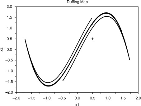
To illustrate the impact of different linearisation strategies for the predictive stage of cycled data assimilation we use the Duffing map [e.g. Saha and Tehri (2010)], which is a discretisation of the Duffing oscillator, and has a cubic non-linearity:33 The system has up to three fixed points along the line x ₁=x ₂: at x ₁=0 and . For a range of choices of a, b, the system is chaotic, e.g. for a=2.75, b=0.15 [eq. (33)] has a leading Lyapunov exponent of 0.615. The first 100 000 iterates of the system with these parameters (started from ) are shown in Fig. 2. Closer scrutiny shows the stable manifold to have an intricate structure which Fig. 2 can only partially reveal.

Fig. 2 100 000 iterates of the Duffing map (33) with a=2.75, b=0.15 starting from (plus sign).

Set D to be the linear part of the Duffing map, i.e.

so where e ₂ is the unit vector (0,1) ^T . If δ is distributed normally with mean zero and variance C, then34 Using these relations we can write down the predictive parts of the TLA filter [eq. (31)] and of the BLA filter [eq. (32)], and with more work also compute exactly the predictive part of the minimum variance filter [eq. (20)]. We find that35 where since P _i∣i is positive semi-definite we have (P _i∣i )₂₂≥0, and therefore as expected is positive semi-definite. is a more complicated symmetric matrix with only the (1, 1) element zero. In view of this, we will setfor real constants β, α.

6.1. Numerical results

We consider the Duffing system eq. (33) with a=2.75, b=0.15 as the truth. The observations are normally distributed about the truth with covariance where σ _o =0.3. There is no model error so Q _i =0. For each assimilation method, the square analysis error is computed for each i and averaged over 100 000 consecutive cycles.

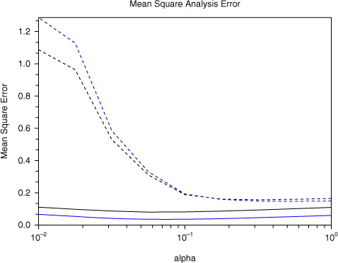
If the minimum variance filter [eqs. (20) and (21)] is used, the mean square analysis error is 0.082. The mean square analysis error for various α (and β=0) using the TLA filter [eqs. (31) and (21)] is shown in solid black and using the BLA filter [eqs. (32) and (21)] in blue in Fig. 3. We have noted that has non-zero off-diagonal elements, but in fact the dependence of the TLA filter on β is very slight – if for each α we find the mean square analysis error for the TLA filter minimised over all real β we obtain the black dotted curve in Fig. 3.

Fig. 3 Mean square analysis error for the Duffing map example, using TLA filter (black) and BLA filter (blue) for various values of the linearisation error parameter α. The dotted curve is the lowest mean square analysis error achievable using the TLA and any value of β.

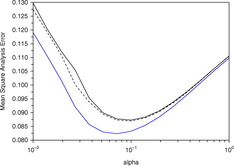
6.2. Remarks

As expected, for a wide range of α the BLA filter has lower analysis errors than the TLA one. When α is large P _i+1∣i in eqs. (31) and (32) is dominated by the large or , the analysis errors become large and increasingly independent of whether the TLA or BLA is used to evolve the posterior covariance from the former time level. In fact, denoting the analyses obtained using eqs. (31) and (32) as, respectively, , , one can show analytically that starting from the same data at i=0 then as α→∞ that for all i.

For small α the analysis errors also become large, as noted in Fisher et al. (2005) and above. Analysis errors are smallest for intermediate values of α, and in fact for α≈0.07 the BLA filter has an analysis error very close to that achieved by the minimum variance filter [eqs. (20) and (21)].

Note the log scale for α. As α→0 analysis errors using both the TLA and BLA become very large, and in the limit there is no guarantee that the BLA filter will have smaller errors than the TLA one, and in fact does not for the parameters a=2.75, b=0.15, σ _o =0.3 as used in Fig. 3.

7. A non-linear generalisation of the Kalman smoother

We will now extend the theory of Sections 4 and 5 from filters to smoothers. As is well known, the EKS is equivalent to a form of 4D-Var, a method of particular interest as it is much the most popular for data assimilation in weather forecasting. For the links between Kalman smoothing and 4D-Var, see Bell (1994).

4D-Var in its simplest form has a fixed prior covariance, often designated B. If one runs 4D-Var this way the choice of B tends to be a large determinant of the quality of the assimilation, rendering comparison of other aspects of the system problematic. To compare the impact of the TL and BL approximations on incremental 4D-Var we therefore prefer to do so in the context of (the variational equivalent to) the EKS.

As with the filters, we first develop a minimum variance smoother from which TLA and BLA smoothers will (in Section 8 below) be derived by making the corresponding linearisations, and which will serve as a benchmark with which to assess the impact of the approximations.

7.1. Minimum variance smoother

The framework is identical to that in Section 4, but now instead of using the observation at time i+1 to find an analysis at time i+1, we are using it to improve the existing analysis at time i. Using exactly the same notation as Section 4, we now seek L _i , d _i depending on and the pdfs of ε _i , w _i , v _i+1 such that if the smoothed analysis is of the form36 then37 is minimised, where the expectation is over ε _i , w _i , v _i+1. As usual, the solution will be independent of A.

The derivation follows the same pattern as Section 4. We suppose the same error structure and definitions as eq. (12), where as before the errors are zero mean and uncorrelated with each other, and again define R _i+1, Q _i by eq. (15). Setting the derivatives of eq. (37) with respect to d _i , L _i to zero, solving the resulting simultaneous equations and using eq. (12) to express all expectations in terms of ε _i , w _i , v _i+1, we obtain after some manipulation38 39 where and P _i+1∣i have the same definitions as in eq. (18), and40 We can easily compute the covariance of the error in the smoothed analysis to be41 which evidently is less than the old one P _i∣i .

Inserting the smoothing stage we have just derived between the prediction and update steps of the minimum variance filter [eqs. (20) and (21)], we obtain the minimum variance smoother of Table 1, where all the expectations are over ε _i ~N(0, P _i∣i ). This algorithm generalises the Kalman smoother in the case the propagating map f _i is non-linear. If f _i is linear, then it simplifies to the usual Kalman smoother, and if f _i is non-linear and we replace by its TL approximation we obtain the usual form of the EKS, a point we amplify on in Section 8 below.

Table 1 Minimum variance smoother

Given first guesses :

For i=0,1, …

Predict:

Smooth:

Update:

End For i

8. Form of smoother where the forecast map is linearised using the TLA or BLA and variational equivalents

In the same way that in Section 5 we derived TLA and BLA filters from the minimum variance filter, we will now derive TLA and BLA smoothers from the minimum variance smoother of Table 1, by replacing wherever it appears in Table 1 by expansions based on the TL and BL approximations. By examining the impact of these approximations on , P _i+1∣i and U _i in the minimum variance smoother, we can compare the impact of making the TLA and BLA on the quality of the data assimilation system.

If in Table 1 we replace by its first-order Taylor expansion [eq. (22)], then and P _i+1∣i are as given by eq. (23). The only new equation is42 Similarly, an expansion based on the BLA [eq. (25)] yields and P _i+1∣i as given by eq. (26), the only new equation is43 Interestingly, there is no term on the right hand side of eq. (43), as by virtue of eq. (6) it vanishes. Thus, in the smoother case use of the BLA has not only the advantages over the TLA listed in (c) and (d) of Section 5, but removes all approximation in U _i .

In summary, the smoother using the BLA is as given by Table 2. The smoother using the TLA is the same with , , replaced by respectively , , .

Table 2 Smoother using the BLA

Given first guesses :

For i=0,1,…

Predict:

Smooth:

Update:

End For i

We can identify three advantages of the BLA over the TLA for the smoother. Like the BLA filter in Section 5, use of the BLA leads to no approximation in the new prior compared with the minimum variance smoother, and the approximation to the prior covariance P _i+1∣i is not dependent on the instantaneous derivative. Furthermore, use of the BLA has the additional advantage that U _i is unapproximated compared with the minimum variance smoother.

8.1. Variational equivalents of the smoother

As discussed at the beginning of Section 7, a key motivation behind extending our study from filters to smoothers is the latter's well known equivalence to forms of 4D-Var (see e.g. Bell (1994)). The non-linear smoother of Section 7 has no immediate variational equivalent, but its TLA and BLA linearisations derived above do, at least so long as , are invertible. Set44 If the state vector is of length n the Hessian (i.e. second derivative) of J in eq. (44) is a matrix of size 2n×2n. By computing its inverse in block form, one may show that the BLA smoother of Table 2 above is identical to the algorithm shown in Table 3, where [..]₁₁ and [..]₂₂ refer respectively to the upper left and lower right n×n submatrices. Note that in this version of incremental 4D-Var the background error covariance is cycled, instead of the static background error covariance used in early implementations.

Table 3 Variational form of smoother using the BLA

Given first guesses :

For i=0,1, …

Find which minimise (44)

End For i

Clearly the variational equivalent of the TLA smoother is as given by eq. (44) and Table 3 with , , replaced by respectively , , .

The matrix in the last line of eq. (44) has appeared frequently in this article, as is to be expected given that from eqs. (12) and (25) we have . As linearisation error and model error w _i are supposed uncorrelated the covariance of their sum is , which is parametrised as . One notable difference between the two errors making up this sum is that model error is a property solely of the model, while linearisation error is a property of the whole forecast-analysis system.

To obtain the strong constraint form of the variational smoother we will need both Q _i and to tend to zero. In the limit as finding δ _i , δ _i+1 which minimise eq. (44) is equivalent to finding δ _i which solves the familiar strong constraint 4D-Var problem:45 followed by

9. Example of smoothers using the TL and BL approximation

We use the BLA and TLA smoothers of Section 8, which we have seen are equivalent to a form of incremental 4D-Var, to assimilate data into the Duffing system of Section 6 (Example 1) and a roughened version (Example 2).

9.1. Example 1: standard version of Duffing map

We assimilate noisy observations into the Duffing map of Section 6, with the same parameters as there: a=2.75, b=0.15, σ _o =0.3 and with no model error, and for both TLA and BLA filters/smoothers a parametrisation of linearisation error of the formAs for the filters in Section 6 we can easily compute exact analytic expressions for all the quantities required for the TLA and BLA smoothers of Section 8. The mean square analysis error obtained for 100 000 consecutive cycles is shown in Fig. 4, using the TLA and BLA filters of Section 5 (black), and the TLA and BLA smoothers of Section 8 (blue). Dotted curves use the TLA and solid curves use the BLA. As we have noted, the smoothers are equivalent to a form of 4D-Var.

Fig. 4 Mean square analysis error for the Duffing map example for various values of the linearisation error parameter α. Filters are in black and smoothers in blue. Dotted curves use the TLA and solid curves use the BLA.

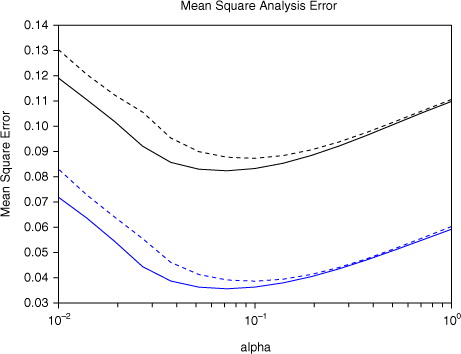
As expected the smoothers outperform the filters. We also see that use of the BLA outperforms use of the TLA, even in this smooth slowly varying map for which the TLA is well-suited. However, the context for which the BLA was most intended is in systems where the propagating map varies rapidly on the scale of the increments, as in the next example.

9.2. Example 2: ‘roughened’ version of Duffing map

To illustrate the use of the BLA in cases where the derivative is unrepresentative of variation in the propagating map f _i on the scale of the increments, e.g. because of the presence of small scales, we consider a roughened version of the Duffing map.

If the greatest integer less than or equal to a real scalar x is denoted floor(x), for positive integer p and any real x setThus the graph of x→[x] ^p is a ‘staircase’ of square steps of step-size 1/p . Note that ∣x−[x] ^p ∣≤1/p for any x, and so as p→∞ we have ∣x−[x] ^p ∣→0 uniformly in x.

We now define a ‘roughened’ version of the Duffing map as46 This then is a roughened or pixelated version of the Duffing map which converges in the C ⁰ norm to the Duffing map as p→∞. It is still chaotic for a=2.75, b=0.15, at least if p is larger than about 50. Note that for any p the derivative of g ^p is47 so is zero except in the (2,2) component.

As before we can compute analytic expressions for all the quantities required for the TLA and BLA smoothers of Section 8. The mean square analysis error (averaged over 30 000 consecutive assimilations) for the roughened Duffing map with a=2.75, b=0.15, p=100 is shown in Fig. 5 using the TLA and BLA filters (black) and smoothers (blue), where dotted curves use the TLA and solid curves use the BLA.

Fig. 5 Mean square analysis error in roughened Duffing map (with p=100) for various values of the linearisation error parameter α. Filters are in black and smoothers in blue. Dotted curves use the TLA and solid curves use the BLA.

Given the form of eq. (47) it is no surprise that the assimilation methods which use the TLA struggle. Errors for the TLA filter are very large and the smoother is no better than the filter. Indeed, in view of eq. (47) we cannot expect that iterating the predict and smooth stages of the TLA smoother for the same i (equivalent to iterating the outer loop in incremental 4D-Var) will give any benefit, and this is confirmed by experiment. On the other hand when the BLA is used the errors are much lower, and (comparing the solid curves in Figs. 4 and 5) are in fact almost unaffected by the transition from smooth to roughened Duffing map.

It is worth noting that this example does not depend critically on the discontinuities in the construction of g ^p . For ∈(0,1), let be a C^∞ ‘cut-off’ function: for x≤0, for x≥, is monotonically decreasing for 0<x<∈, and all derivatives of vanish at x=0, . If one then setsthen floor is a smooth function which ‘rounds off’ the steps of the function floor and converges to floor as →0. Now define in terms of floor and in terms of . Then we could repeat the example using smooth , and for sufficiently small the results will not differ appreciably from those we found using g ^p .

10. Summary and remarks

To form a local linear approximation for finite-sized perturbations of a non-linear function f the tangent-linear approximation may be inappropriate. The best linear approximation is a readily calculable function of f and the pdf of the increments. It does not require differentiability of f. The fact that the best linear approximation is independent of the smoothness of f makes it particularly attractive for the linearisation of physical parametrisations, and as we saw in the cloud example the reduction in linearisation error in such cases can be considerable.

The main focus of the article is on applying the BLA in the data assimilation cycle. As a benchmark we use minimum variance filters and smoothers which are non-linear generalisations of Kalman filters and smoothers. In our context, the predictive part of the minimum variance filter is equivalent to evolving the posterior pdf by the Chapman–Kolmogorov equation, and approximating the new prior pdf by a Gaussian one with the same first two moments.

If into the minimum variance filter we replace the forecast map by its TL approximation we obtain the usual EKF. If instead we use the BL approximation, we noted two advantages, the first being that the prior is unapproximated compared with the minimum variance filter. This occurs because the expectation of f _i is also the expectation of the BLA of f _i . The covariance of the prior in the minimum variance filter involves the expectation of the square of f _i , so using the BLA of f _i leads to an approximation in this. However, the second advantage of the BLA is that, by contrast with the TLA, the error in this approximation is bounded independently of the vagaries of the instantaneous derivative.

The first advantage removes an approximation while the second greatly reduces the damage a bad approximation can do. Their relative importance tends to depend on how poor the TL approximation is. If it is quite good, the main advantage is in the improved prior itself. On the other hand, if the TL approximation is poor the improved prior covariance of the BL filter becomes very important.

Interestingly, while the BL approximation yields a prior covariance which is normally closer to the benchmark than that from the TLA, it always underestimates it, by the covariance of the linearisation error. This means that allowing for linearisation error, which is already known to be important for the EKF using the TLA, is at least as important if the BLA is used. In the latter case, this involves adding an estimate of the covariance of linearisation error to the prediction of the covariance of state error. This is especially important in the perfect model context. With an imperfect model the approximations made in parametrising the true model error covariance may in some cases render separate allowance for linearisation error unnecessary.

We also developed a minimum variance smoother. Inserting the BL and TL approximations into this, we see that BLA smoothers have the same advantages over TLA smoothers that the filters do, and additionally that the smoothing step in the BLA smoother is unapproximated compared with the minimum variance smoother.

We have concentrated on non-linearity in the forecast map, but there is no difficulty (the details are in an appendix) applying the same principles to non-linearity in the observation operator.

In some large-scale applications the computation of f ⁽⁰⁾ and f ⁽¹⁾ will need to be done approximately, for example by use of an ensemble of forecasts from perturbed analyses which may already exist for ensemble forecasting. Alternatively, in some instances one may be able to get a useful approximation to f ⁽¹⁾ by using a climatological pdf of perturbations, and so f ⁽¹⁾ can be computed entirely off-line. One can interpret the ‘perturbation forecast’ model approach of Lorenc (1997) and adopted at the Met Office as being in this spirit.

The analysis in this article has been for filters and smoothers in their discrete form, but a similar approach can be followed in the continuous case, by using the BLA in place of the TLA when linearising the non-linear terms in the PDEs describing the forecast model.

11. Acknowledgments

The author thanks Andrew Lorenc for useful discussions, and three referees appointed by Tellus for their careful reviews and helpful suggestions.

Appendix

A.1. Equivalence of the minimum variance algorithm of Section 4 and optimal Bayesian dynamic state estimation with Gaussianised pdfs

We use the framework described at the beginning of Section 4 and in particular in eq. (12), and suppose also that observation and model errors are Gaussian, i.e.A1 As usual we denote the conditional pdf of x _i given y ₁,…y _j by or . We show that the minimum variance filter of Section 4 is equivalent to optimal Bayesian dynamic state estimation, if in the latter case each prior pdf is approximated by a Gaussian with the same first two moments.

In Bayesian dynamic state estimation (e.g. Arulampalam et al. (2002)), Bayes’ ruleA2 is used to form the posterior pdf p(x _i∣i ) from the prior pdf p(x _i∣i−1). With our assumption [eq. (A1)] this posterior will be Gaussian if p(x _i∣i−1) is. The pdf p(x _i∣i ) is then evolved forward to form the prior pdf p(x _i+1∣i ) at the next time level byA3 Equation (A3) can be viewed as a form of the Chapman–Kolmogorov equation, and we follow Arulampalam et al. (2002) by referring to it as such. Observe that by virtue of eqs. (12) and (A1) the transition pdf p(x _i+1∣ x _i ) used in (A3) is Gaussian with mean f _i (x _i ) and covariance Q _i , so if f _i is non-linear then p(x _i+1∣i ) is non-Gaussian even if p(x _i∣i ) was Gaussian.

Suppose that the prior pdf p(x _1∣0) is Gaussian with mean and covariance . Applying Bayes Rule [eq. (A2)], we find is Gaussian with mean and covariance given by eq. (21) with i=0, so the optimal Bayesian approach and the minimum variance filter of Section 4 coincide at the outset.

Now suppose inductively that at the ith stage the posterior pdf is Gaussian with mean and covariance as given by eq. (21). Then using eq. (12), the definition of conditional mean and the inductive hypothesis it follows that the conditional mean of given A4 where the expectation on the right hand side is over . Denoting by , we find by similar means that the conditional covariance of given A5 where again the expectation on the right hand side is over . Evidently the right hand sides of eqs. (A4) and (A5) are identical to the expressions for and in eq. (20). If we now replace by a Gaussian pdf with mean [eq. (A4)] and covariance [eq. (A5)] and use this modified pdf in Bayes’ rule [eq. (A2)], we find is Gaussian with mean and covariance given by eq. (21). By induction, it follows that if at every stage we approximate the prior pdf given by the Chapman–Kolmogorov equation [eq. (A3)] by a Gaussian one with the same mean and covariance, then the resulting prediction-update cycle coincides with the minimum variance filter of Section 4.

A.2. The BLA filter – existence, comparison with UKF, and extension to non-linear observation operators

A.2.1. Conditions for the existence of the filter using the BLA.

We compare the TLA and BLA filters [eqs. (31) and (32)] in terms of what restrictions must be placed on f _i and the other quantities involved for the filters to exist. Clearly, if the TLA is used as in eq. (31) then we need f _i to be differentiable. For the BLA filter [eq. (32)], f _i does not even need to be continuous, which can be a significant advantage. We merely require the existence ofwhere the expectations are over . For this, we require (a) that for every i the expectations and exist, which is ensured under very mild restrictions on f _i by virtue of the rapidity with which a Gaussian pdf p(x) tends to zero as , and (b) the non-singularity of . Suppose is non-singular. From eq. (32) we see that is a sum of three positive semi-definite matrices,and so if is non-singular then so is so long as at least one of , or is. From eq. (21) we have . Since we may assume R _i is non-singular it follows that if is non-singular then so is . Inductively, is non-singular for all i so long as for every i at least one of , or Q _i is non-singular.

A.2.2. Remarks on the unscented Kalman filter and comparison with the BLA filter.

Another filter, which like eqs. (31) and (32) is based on eq. (20) for its predictive part, is the unscented Kalman filter (UKF) of Julier and Uhlmann (1997). If the state space has dimension n, this estimates the expectations in eq. (20) by evaluating f _i at 2n+1 carefully chosen ‘sigma-points’. Julier et al. (2000) compute Taylor series expansions of the mean and covariance as predicted by eq. (20) and compare with similar expansions for the standard EKF [i.e. using the TLA as in eq. (31)] and the UKF, where in all cases, as in eq. (20), the analysis errors have a Gaussian distribution. They find that using the TLA the mean is correct to first order and the covariance to third order, while using the UKF the mean is correct to second order and the covariance again to third order. For the BLA filter, we have already noted that in eq. (32) is identical to the value given by eq. (20), i.e. the mean is correct to every order, and by a similar analysis to that in Julier et al. (2000) we find that the BLA filter also gives third-order accuracy for the covariance. More importantly, we have seen that the departure of the covariance of the BLA filter from the benchmark [eq. (20)] is bounded by [eq. (30)].

A.2.3. Note on extension of the BLA filter to non-linear observation operators.

For simplicity we have taken the observation operator to be the identity. More generally the last line of eq. (12) takes the formwhere the observation operator may be non-linear. In this case, one can repeat the analysis of Section 4 to generalise our minimum variance filter [eqs. (20) and (21)]. One finds that eq. (20) is unchanged but the update equations in eq. (21) becomeA6 where denoting by we haveA7 A8 A9 The BLA of has the form and can either be computed directly, or approximated by first computing the BLA of by eq. (25), and then computing the BLA of h _i+1 applied to this. Either way we can insert this linear approximation and eq. (25) into eqs. (A7)–(A9), and thereby generalise the BLA filter to allow for non-linear observation operators.

References

- Arulampalam M. S , Maskell S , Gordon N , Clapp T . A tutorial on particle filters for online nonlinear/non-Gaussian Bayesian tracking. IEEE Trans. Signal Process. 2002; 50: 174–188.
- Bell B. M . The iterated Kalman smoother as a Gauss–Newton method. SIAM J. Optim. 1994; 4: 626–636.
- Errico R. M , Raeder K. D . An examination of the accuracy of the linearization of a mesoscale model with moist physics. Q. J. Roy. Meteorol. Soc. 1999; 125: 169–195.
- Fisher M , Leutbecher M , Kelly G. A . On the equivalence between Kalman smoothing and weak-constraint four-dimensional variational data assimilation. Q. J. Roy. Meteorol. Soc. 2005; 131: 3235–3246.
- Gelb A . Applied Optimal Estimation. 1974; MIT Press, Cambridge, MA..
- Jaswinski A. H . Stochastic Processes and Filtering Theory. 1970; Academic Press, New York..
- Julier S. J , Uhlmann J. K , Kadar I . A new extension of the Kalman filter to nonlinear systems. Proc. SPIE Vol. 3068, Signal Processing, Sensor Fusion, and Target Recognition VI. 1997; Orlando, FL: SPIE. 182–193.
- Julier S , Uhlmann J , Durrant-Whyte H. F . A new method for the nonlinear transformation of means and covariances in filters and estimators. IEEE Trans. Automat. Contr. 2000; 45: 477–482.
- Lawless A. C , Gratton S , Nichols N. K . An investigation of incremental 4D-Var using non-tangent linear models. Q. J. Roy. Meteorol. Soc. 2005; 131: 459–476.
- Lorenc A. C . Development of an operational variational assimilation scheme. J. Met. Soc. Japan. 1997; 75: 339–346.
- Lorenc A. C , Payne T. J . 4D-Var and the butterfly effect. Q. J. Roy. Meteorol. Soc. 2007; 133: 607–614.
- Luca M. B , Azou S , Burel G , Serbanescu A . On exact Kalman filtering of polynomial systems. IEEE Trans. Circ. Syst. 2006; 53: 1329–1340.
- Sage A. P , Melsa J. L . Estimation Theory with Applications to Communications and Control. 1971; McGraw Hill, New York..
- Saha L. M , Tehri R . Applications of recent indicators of regularity and chaos in discrete maps. Int. J. Appl. Math. Mech. 2010; 6: 86–93.
- Smith R. N. B . A scheme for predicting layer clouds and their water content in a general circulation model. Q. J. Roy. Meteorol. Soc. 1990; 116: 435–460.