Weather Research and Forecasting Model simulations of extended warm-season heavy precipitation episode over the US Southern Great Plains: data assimilation and microphysics sensitivity experiments

Abstract

This study examines eight microphysics schemes (Lin, WSM5, Eta, WSM6, Goddard, Thompson, WDM5, WDM6) in the Advanced Research Weather Research and Forecasting Model (WRF-ARW) for their reproduction of observed strong convection over the US Southern Great Plains (SGP) for three heavy precipitation events of 27–31 May 2001. It also assesses how observational analysis nudging (OBNUD), three-dimensional (3DVAR) and four-dimensional variational (4DVAR) data assimilation (DA) affect simulated cloud properties relative to simulations with no DA (CNTRL). Primary evaluation data were cloud radar reflectivity measurements by the millimetre cloud radar (MMCR) at the Central Facility (CF) of the SGP site of the ARM Climate Research Facility (ACRF). All WRF-ARW microphysics simulations reproduce the intensity and vertical structure of the first two major MMCR-observed storms, although the first simulated storm initiates a few hours earlier than observed. Of three organised convective events, the model best identifies the timing and vertical structure of the second storm more than 50 hours into the simulation. For this well-simulated cloud structure, simulated reflectivities are close to the observed counterparts in the mid- and upper troposphere, and only overestimate observed cloud radar reflectivity in the lower troposphere by less than 10 dBZ. Based on relative measures of skill, no single microphysics scheme excels in all aspects, although the WDM schemes show much-improved frequency bias scores (FBSs) in the lower troposphere for a range of reflectivity thresholds. The WDM6 scheme has improved FBSs and high simulated-observed reflectivity correlations in the lower troposphere, likely due to its large production of liquid water immediately below the melting level. Of all the DA experiments, 3DVAR has the lowest mean errors (MEs) and root mean-squared errors (RMSEs), although both the 3DVAR and 4DVAR simulations reduced noticeably the MEs for seven of eight microphysics schemes relative to CNTRL. Lower-tropospheric θ _e and convective available potential energy (CAPE) also are closer to the observations for the 4DVAR than CNTRL simulations.

• data assimilation
• microphysics sensitivity
• WRF evaluation
• MMCR-equivalent reflectivity simulation
• Southern Great Plains

To access the supplementary material to this article, please see Supplementary files under Article Tools online.

1. Introduction

Cloud-resolving regional climate models are important tools to study climate processes and increase our understanding of the interactions between clouds, radiation and large-scale atmospheric dynamics (e.g. Ferrier et al., 1995; Tao et al., 2003; Hong et al., 2004; Leung et al., 2006; Wu et al., 2008). However, even in highly sophisticated models, the representation of clouds remains a challenge (e.g. Tao et al., 2003; Morrison and Grabowski, 2007) and is a major source of uncertainty in climate change projections (e.g. Dong et al., 2005; Stensrud, 2007, pp. 260–261; Otkin and Greenwald, 2008). Improving the accuracy of cloud treatment in large-scale models is essential to reduce uncertainties in future climate projections (e.g. Luo et al., 2006) or increase the reliability of high-impact precipitation forecasts in convection-resolving models (Hong et al., 2009). Systematic studies are needed to quantify model errors and characterise their sensitivities in greater detail (e.g. Luo et al., 2006; Weisman et al., 2008).

The Weather Research and Forecasting Model (WRF; Skamarock et al., 2008), which was developed as a community model, has had an exponential increase in the number of users over the past few years (e.g. Warner, 2011). It has been used in many applications, from high-resolution real-time weather forecasting (e.g. Kain et al., 2006; Weisman et al., 2008; Schwartz et al., 2009; Clark et al., 2010) to regional climate down-scaling (e.g. Zhang et al., 2009; Qian et al., 2010). WRF is also widely used to evaluate the impact of microphysical and convection schemes (e.g. Gallus and Bresch, 2006; Jankov et al., 2007, 2009; Bukovsky and Karoly, 2009), planetary boundary layer (PBL) physics (e.g. Otkin and Greenwald, 2008; Hu et al., 2010), and data assimilation (DA) procedures (e.g. Weisman et al., 2008; Wheatley and Stensrud, 2010). Most studies concur that DA improves the timing and intensity of simulated convective storms. Furthermore, it was suggested that both PBL and cloud microphysics schemes exert strong influence on the spatial distribution and physical properties of simulated cloud fields. However, model sensitivities to these physical schemes are dependent on initialisation processes (e.g. Jankov et al., 2007) or were not the major contributor to short-term forecast errors (Weisman et al., 2008). In real-time forecasting and model sensitivity studies, previous model verification analyses focused on the horizontal structure and temporal evolution of convection.

To identify model deficiencies, model performance evaluation should include characterisation of model systematic errors related to the vertical structure of convection. The US Department of Energy's ARM Climate Research Facility (ACRF) in the Southern Great Plains (SGP) makes detailed measurements of radiation and clouds at its Central Facility site (CF; 36.6°N, 97.5°W; Stokes and Schwartz, 1994; Ackerman and Stokes, 2003). These continuous, high temporal resolution physical measurements permit detailed comparison of WRF simulations of clouds and convection with observations.

Towards that end, we examine the ability of the Advanced Research WRF (ARW) model to reproduce the observed vertical structure of convection and clouds in the vicinity of the CF for the warm-season heavy precipitation events of 27–31 May 2001. The main objectives are to evaluate eight WRF microphysics schemes, emphasising their partitioning of water species and convection intensity and timing, and assessing the impact of DA on simulated Ka-band cloud radar reflectivity. Comprehensive characterisations of cloud-resolving simulations and quantification of associated model errors and sensitivities are needed for improved representation of clouds and convection in regional models. This challenge is a research objective of the Atmospheric System Research (ASR) Program of the US Department of Energy (US Department of Energy, 2010, p. 14). These objectives have received little attention, either for WRF or other cloud-resolving regional climate models. Zhu et al. (2012, p. 2) therefore noted that ‘the robustness of state-of-the-art regional models in simulating convective systems at the cloud resolving scale has yet to be extensively evaluated’.

2. Data and methodology

2.1. Observational data

Observational data are from or for the ACRF SGP site (Fig. 1) for 27–31 May 2001. Hourly precipitation rates were measured by 15 Surface Meteorological Observation Systems (SMOSs, Fig. 1). Millimetre Cloud Radar (MMCR) reflectivity, ice water content (IWC) and liquid water content (LWC) data were obtained from Mace et al.'s (2006) SGP Atmospheric State, Cloud Microphysics and Radiative Flux Divergence value-added products (VAPs). These data document the hourly progression of cloud characteristics in the atmospheric column over the SGP CF. Mace et al.'s (2006) VAPs have a vertical grid spacing of 90 m. All the above data were used to evaluate model results.

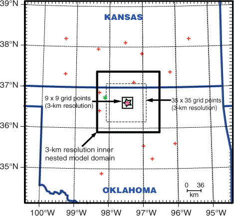
Fig. 1 Location map. Boundaries enclose WRF-ARW outer model domain, with thick broken line delineating the inner 3-km grid spacing nested domain centred over the Southern Great Plains (SGP) Central Facility (CF). Dark (light) dotted square surrounding the CF demarcates 9×9 (35×35) grid points over which model results and derived statistics were averaged. Locations are given for SGP Surface Meteorological Observation System (SMOS) instruments (red crosses) and CF rawinsonde station (centre of star) used for data assimilation (DA), and for WSR-88D radar at Vance AFB (green asterisk) used for comparison.

The MMCR reflectivity data were measured by a zenith-pointing cloud radar operating at 35-GHz (8.7-mm wavelength, Ka-band) frequency. The radar system is designed to maximise radar detection of a wide range of cloud conditions by providing excellent sensitivity, resolution and flexibility of operating options (Clothiaux et al., 2000). The cloud reflectivity profiles were reconstructed from the four MMCR data collection modes. Significant radar echoes were identified and distinguished from non-cloud radar returns in the boundary layer using cloud base measurements recorded by ceilometers (Mace et al., 2006). While millimetre-wave radars can provide details of non-precipitating cloud characteristics, they suffer severe attenuation in heavy precipitation events. Fortunately, total attenuation occurred at few times during our study period and all subsequent statistical analyses involving MMCR data excluded such missing data.

To provide a larger scale setting, S-band reflectivity data were also used from the NOAA/DoD Weather Surveillance Radar-1988 Doppler (WSR-88D) network. The WSR-88D Level-III composite reflectivity data from the Vance Air Force Base radar (~60-km west-northwest of the SGP CF) were obtained from the NOAA National Climatic Data Center website (http://has.ncdc.noaa.gov). These reflectivity data (mm⁶ m⁻³) were sampled every hour and interpolated onto WRF model grids (Fig. 1) for evaluation.

Although the scattering and absorption of millimetre (e.g. Ka-band) and microwave (e.g. S-band) radiation by any hydrometeor smaller than about 100 µm can be treated using the Rayleigh approximation, the scattering and absorption of precipitation particles must be investigated using the Mie functions (Lhermitte, 1987, 1990; Raghavan, 2003, p. 71). Therefore, simulated reflectivities for both the Ka-band and S-band radars were computed using the full Mie calculations, as discussed below. Attenuations from both atmospheric gases and hydrometeors were evaluated to account for loss of radiation.

2.2. WRF model simulation design

The Advanced Research WRF (ARW) model version 3.1 (Skamarock et al., 2008) was used to simulate the warm-season SGP high precipitation case of 27–31 May 2001. Skamarock and Klemp (2008) provide details of the numerical schemes. This version is dated April 2009, and here has one-way nested domains centred on the SGP CF and 41 vertical levels, including 10 levels below 2 km. The outer domain covers 61×61 grid points, with 9-km grid spacing (Fig. 1). Located at the centre of the outer domain, the inner domain spans 55×55 grid points at 3-km grid spacing. A time step of 10 seconds was used for the nested domain. Initial and lateral boundary conditions were obtained from the National Centers for Environmental Prediction (NCEP) Final Analysis data (http://rda.ucar.edu), which have 6 hours and 1° latitude/longitude resolutions. The WRF-ARW model was initialised at 0600 UTC 27 May 2001 and integrated for 108 hours until 1800 UTC 31 May 2001.

The land-surface model (LSM) employed in this study is based on the MM5 five-layer soil temperature model. It provides heat and moisture fluxes as a lower boundary condition for the Yonsei University PBL scheme (Hong et al., 2006). Model radiation options used were the rapid radiative transfer model long-wave radiation scheme (Mlawer et al., 1997) and the MM5 short-wave radiation scheme (Dudhia, 1989). The Kain–Fritsch cumulus parameterisation (Kain and Fritsch, 1993) was activated for the outer (coarse) domain. No convective parameterisation was employed for the 3-km inner-nested domain.

As grid-resolvable cloud and precipitation processes are governed by treatments of microphysical processes, this study uses and assesses the cloud and convection representations in the following eight WRF microphysics schemes that are documented in detail in Table 1: (1) Purdue–Lin (henceforth termed Lin; Lin et al., 1983; Chen and Sun, 2002); (2)–(5) WRF Single/Double-Moment 5-class/6-class (WSM5/WSM6, WDM5/WDM6; Hong et al., 2004, 2009; Hong and Lim, 2006); (6) Eta-Ferrier (Eta; Ferrier et al., 2002); (7) Goddard cumulus ensemble (GCE) model (Goddard; Tao et al., 2003; Lang et al., 2007); and (8) Thompson et al. (Thompson; Thompson et al., 2008). The WSM5 and WDM5 schemes predict five water species, including water vapour, cloud water, rain, ice and snow condensates. The Eta scheme predicts changes in water vapour and condensate in the forms of cloud water, rain and precipitation ice (Hong et al., 2009). The remaining five schemes include graupel as an extra hydrometeor class. In addition to predicting hydrometeor mixing ratios, the WDM5 and WDM6 microphysics schemes predict the number concentrations of rain and cloud water, whereas the Thomson microphysics scheme predicts the number concentrations for rain and ice condensates.

Table 1. Particle size distribution (PSD) characteristics employed for simulated radar experiments

Experiment or microphysics scheme	Water species	Functional form	N 0/intercept parameter	λ (slope)	m(D)=αD ^β or constant density	Remarks	References
Cloud	Monodisperse	N c=1×10^8		Spherical particles with	^R1 Rutledge and
Rain	Exponential	8×10^6	Diagnosed	ρ w	constant density	Hobbs (1983)
Lin	Snow	Exponential	3×10^6	Diagnosed	ρ s=100
Graupel	Exponential	4×10^4	Diagnosed	ρ g=400
Ice*	Monodisperse	N i from A13 of R1
Cloud	Monodisperse	N c=3×10^8		ρ w	Mass-dependent ice	^R2 Hong et al. (2004)
Rain*	Exponential	8×10^6	Diagnosed	ρ w	concentration
WSM5	Snow*	Exponential	Eq. 6 of R2	Diagnosed	ρ s=100
Graupel	NOT	USED
Ice*	Monodisperse	N i from Eq. 5c of R2		α=1/11.9^2, β=2
Cloud*	Monodisperse	N c=1×10^8		ρ w	Mass-Lookup table	^R3 Houze et al. (1979)
Rain*	Exponential	Rain content dependent		ρ w	based on R3
Eta	Snow*	Exponential	Lookup table based on R3
Graupel	NOT	USED
Ice	NOT	USED
Cloud	Same as WSM5				Temperature dependent
Rain*	Same as WSM5				snow intercept
WSM6	Snow*	Same as WSM5				parameter as in WSM5
Graupel	Exponential	4×10^6	Diagnosed	ρ g=500
Ice*	Same as WSM5
Cloud	Monodisperse	N c=1×10^8		ρ w	Spherical particles with	^R4 Thompson
Rain	Exponential	8×10^6	Diagnosed	ρ w	constant diameter	et al. (2008)
Goddard	Snow	Exponential	1.6×10^7	Diagnosed	ρ s=100
Graupel	Exponential	4×10^6	Diagnosed	ρ g=400
Ice*	Monodisperse	N i from A13 of R1
Cloud*	Generalised gamma	N c=3×10^8	Eq. A4 of R4	ρ w	Number concentrations for rain and ice are	^R5 Morrison et al. (2009)
Rain*	Exponential	Eq. 3 of R5	Diagnosed	ρ w	predicted
Thompson	Snow*	Eq. 1 of R4	Parameters from R6		α=0.069, β=2
Graupel*	Exponential	Mixing ratio-dependent (R4)		ρ g=400	^R6Field et al. (2005)
Ice*	Exponential	Eq. 3 of R5	Diagnosed	ρ i=890
Cloud*	Generalized gamma	Diagnosed	Eq. 2 of R7 (νc=1, α c=3)	ρ w	Number concentrations for cloud and rain are	^R7 Lim and Hong (2010)
Rain*	Generalized gamma	Diagnosed	Eq. 2 of R7 (νr=2, α r=1)	ρ w	predicted
WDM5	Snow*	Exponential	Eq. 6 of R2	Diagnosed	ρ s=100
Graupel	NOT USED
Ice*	Same as WSM5
Cloud*	Same as WDM5
Rain*	Same as WDM5
WDM6	Snow*	Same as WDM5
Graupel	Same as WDM5
Ice*	Same as WDM5

For all microphysics-based experiments, the PSDs are used for weather (S-band) and cloud (Ka-band) radar reflectivity simulations. ρ _w is the density of water (1000 kg m⁻³), and ρ _s and ρ _g are densities of snow and graupel, respectively. The * in the Water Species column indicates the relevant QuickBeam routines for the corresponding condensate were modified or replaced by code snippets from the WRF-ARW microphysics routines to implement WRF-ARW-consistent microphysical attributes. R1–R7 in centre of table indicate references given in the extreme right-hand column. See text for further details.

The QuickBeam radar simulation package (Haynes et al., 2007) was used, modified as indicated below and in Table 1, to convert WRF-ARW-simulated profiles of thermodynamic and hydrometeor variables to the equivalent of radar reflectivities measured by the MMCR (35 GHz/8.7 mm) and WSR-88D (3 GHz/10 cm). The original QuickBeam simulation package has five preset particle size distribution (PSD) functions and accounts for attenuation of the radar beam by both atmospheric gases and hydrometeors. It computes particle absorption and scattering properties using full Mie equations (e.g. Lhermitte, 2002, p. 194; Raghavan, 2003, p. 62). To implement WRF-ARW-consistent PSD forms and mass–size relationships in QuickBeam, we modified the PSD and mass–size relationships for several water species, as in Table 1. The resulting relationships are employed to compute the equivalent radar reflectivity factor (Z _e) of simulated clouds and precipitating particles for radars operating at 35 and 3 GHz frequencies, using the Mie backscattering cross sections (e.g. Lhermitte, 2002, p. 194; Raghavan, 2003, p. 63). Unmodified from the QuickBeam package, signal attenuations from atmospheric gases are computed following Liebe (1985), while attenuations from hydrometeors are evaluated by calculating extinction cross sections using the Mie equations (e.g. Lhermitte, 2002, pp. 197–214; Raghavan, 2003, pp. 85–89). The equivalent radar reflectivity factor (Z _e, hereafter termed reflectivity, in mm⁶ m⁻³ or dBZ) for the 35 GHz (Z _ek) and 3 GHz (Z _es) radars was calculated with reference to water (e.g. Lhermitte, 1990; Houze, 1993, pp. 111–112; Raghavan, 2003, p. 71) using , where λ is the radar wavelength, ∣K∣² is taken as 0.93 for liquid water (as used for MMCR and WSR-88D radars), and the radar reflectivity η is the backscattering cross section per unit volume obtained from the above Mie application.

The impact of these relatively small domain sizes was assessed by conducting an experiment using a much larger outer domain of 165×165 grid points (same 9-km horizontal grid spacing) with a similarly expanded nested domain of 163×163 grid points (same 3 km grid spacing) centred on the CF. It was found that the timing and general cloud patterns of the simulated near CF area-averaged reflectivities (for surrounding 9×9 grid points, Fig. 1) are fairly similar for the nested domains containing 163×163 vs. 55×55 grid points. A major difference between the two simulations is that the large domain (163×163) simulation produced a stronger reflectivity near the end of the simulation. Considering the large computational resource requirement for the large domain and the appreciable similarity in reflectivity at the centre of the domain, we are justified in using the smaller 55×55 nested domain for evaluating the WRF-ARW DA and microphysics simulations.

A 3-km horizontal grid spacing may not be sufficient to resolve individual convective cells and capture the full spectrum of convective motions. However, Bryan and Morrison (2012) concluded that a horizontal grid spacing from 0.25 to 4 km can be used for microphysical sensitivity tests, although slower evolution and larger convective cells should be expected at the 4-km grid spacing. While decreasing the grid spacing from 1 km to a few hundreds of metres can change details of the simulation and modify the evolution of features that are important to severe weather warning operations, the overall storm structure and cloud properties should not be greatly affected (e.g. Stensrud, 2007, pp. 262–263; Morrison et al., 2009).

Some of the above WRF-ARW v.3.1 experiments were re-run using the most recent version of the model (v.3.4.1, released in August 2012), because of its improved physical parameterisations (microphysics, planetary boundary layer, LSM). Such additional v.3.4.1 simulations were performed using the Lin, WSM6 and Thompson microphysics schemes. However, these new simulations did not reveal any significant differences in the overall evolution of the 27–31 May precipitation episode from that obtained using v.3.1 and presented here. Minor variations between the simulations were attributed at least partly to vertical interpolation differences.

2.3. Evaluation metrics

Verification metrics utilised to compare simulations with observations include correlation, mean error (additive bias, ME), root mean-squared error (RMSE), frequency bias score (FBS) and equitable threat score (ETS). To accommodate a spatial grid point mismatch between simulated and observed variables (e.g. Schwartz et al., 2009; Clark et al., 2010), model-simulated values were averaged over the 9×9 (81) inner domain grid points (27×27 km) immediately surrounding the CF (Fig. 1) and used in all subsequent model verification analyses. All correlations were computed from at least 10 pairs of observed-simulated reflectivity data that were>−60 dBZ, excluding data when the MMCR was severely attenuated. Unless explicitly stated, all reflectivity-related computations were performed on a linear scale (mm⁶ m⁻³). For simulated (Z ^M) and observed (Z ^O) cloud reflectivities, the ME and RMSE were computed following their standard definitions on the errors , over N height–time points (Table 2).

Table 2. Root mean-squared error (RMSE, dBZ) and mean error (ME, dBZ) for eight WRF microphysics simulations of radar reflectivity with (OBNUD, 3DVAR, 4DVAR) and without (CNTRL) data assimilation (DA) for 0600 UTC 27 May–1800 UTC 31 May, 2001 (108-hourly verifications)

		Data assimilation (DA)
		CNTRL		OBNUD		3DVAR		4DVAR
Microphysics		RMSE	ME	RMSE	ME	RMSE	ME	RMSE	ME
Lin	All times	26.4	14.1	26.7	14.6	17.5**	11.1*	22.5	11.8
Initial DA	28.2	16.2	28.5	16.7	16.4**	9.3**	24.2	12.1*
WSM5	All times	18.9	11.4	20.7***	13.9***	17.6	11.7	20.1*	13.7***
Initial DA	20.7	13.8	22.1*	15.8**	18.8*	12.1*	21.8	15.9***
Eta	All times	21.1	12.8	22.2	13.7	17.6***	10.6***	19.2**	10.8***
Initial DA	22.9	15.8	24.0	16.8	14.7***	9.0***	20.7*	12.7**
WSM6	All times	24.2	15.3	24.8	16.2	18.9***	12.5***	24.1	14.9
Initial DA	26.1	18.3	26.7	18.9	20.7***	14.7***	25.5	17.9
Goddard	All times	22.3	15.6	21.2	15.2	19.8**	13.8***	20.4*	14.4**
Initial DA	24.1	17.8	22.8	16.8	21.7*	15.6***	22.5	16.4*
Thompson	All times	18.9	12.4	19.2	11.1**	17.5***	10.1***	17.8***	10.5***
Initial DA	19.3	12.9	20.1	10.6**	18.0*	10.1***	16.7***	9.2***
WDM5	All times	18.0	10.7	19.6**	12.1**	14.7***	6.8***	18.0	9.6
Initial DA	19.6	12.8	20.6	13.5	16.2***	8.4***	19.8	11.4
WDM6	All times	23.1	12.9	24.6	14.4	15.8**	7.3***	22.2	12.0
Initial DA	25.0	15.9	26.5	17.5	16.4***	7.2***	24.2	15.2

Same statistics also were computed for the first 36 h of the data assimilation to assess the immediate data assimilation effects (Initial DA, 36-hourly verifications). To express ME in dBZ, the average departures from the observation (ME_d in mm⁶ m⁻³) were equated to 0 for small departure values between −1 and +1, given by 10*log10(ME_d) for ME_d>1, and given by −10*log10 (−ME_d) for ME_d<−1. Bold values indicate OBNUD, 3DVAR and 4DVAR RMSEs and MEs for which their differences from the corresponding CNTRL values are statistically significant at levels of ≤1% (triple asterisks), ≤5% (double asterisks) and ≤10% (single asterisk) according to a two-tailed ordinary bootstrap test (Section 2.3).

The ETS measures model skill in producing reflectivity exceeding a given threshold after adjusting for chance occurrence (Schaefer, 1990; Jankov et al., 2005; Schwartz et al., 2009). ETS values were calculated for reflectivity thresholds Zt of −35 to +20 dBZ at 1 dBZ intervals using1

and2

where O _Zt (F _Zt ) is the number of height–time points with observed (simulated) reflectivity in excess of threshold Zt,C _Zt is the number of the domain points with observed and simulated reflectivities exceeding Zt, and CHA _Zt is the number of points at which Zt occurs by chance. The ETS varies from −1/3 for worse than chance to 0 for no skill and 1 for perfect skill. In addition, the FBS is the ratio of the frequency of simulated to observed cloud radar reflectivity as follows:3

FBS was evaluated for the same 56 threshold values as the ETS (from −35 dBz to +20 dBZ at 1 dBZ intervals). A perfect FBS score is 1, and a value exceeding (below) 1 indicates model overestimation (underestimation) at that threshold (e.g. Schwartz et al., 2009).

To assess the statistical significance of the above ETSs and FBSs, the 95% confidence intervals (CIs) were calculated using the conventional bootstrap technique (Efron and Tibshirani, 1993, pp. 221–233; Tamhane and Dunlop, 2000, pp. 597–600). In this method, synthetic simulations of 10000 iterations were performed in which the ETS and FBS were calculated from simulated and observed cloud radar reflectivity time series after randomly sampling the original data with replacement. The resulting artificial array is ranked in ascending order, with the 2.5% and 97.5% positions giving the 95% CI for that statistic (e.g. Mullen and Buizza, 2001).

In addition, the conventional bootstrap technique was used for two-sample unpaired hypothesis testing (e.g. Tamhane and Dunlop, 2000, pp. 597–600; Wilks, 2006, pp. 166–170) to identify the statistical significance of a difference metric between simulations with DA and without DA (CNTRL). An achieved significance level (ASL) was obtained from synthetic simulations of 10000 iterations. In these simulations, Z ^M−Z ^O (mm⁶ m⁻³) values were sampled with replacement from a set containing individual DA and corresponding CNTRL Z ^M−Z ^O values, and MEs/RMSEs for the DA and CNTRL were evaluated and their synthetic difference metrics (DA-minus-CNTRL) determined. The resulting two-sided ASL was the fraction of the random ME/RMSE DA-minus-CNTRL differences that were at least as large in absolute value as the actual ME/RMSE DA-minus-CNTRL differences (Table 2). This ASL gives probability values p for two-sided statistical significance of ME and RMSE differences between the DA and CNTRL simulations.

2.4. Data assimilation

The impact of DA on WRF-ARW-simulated cloud microphysical and convection characteristics was examined by assimilating hourly SGP Extended Facility (EF) surface measurements and 6-hourly rawinsonde data from the CF (Figs. 1 and 2). The assimilation was performed using 3DVAR and 4DVAR systems (Barker et al., 2004) for the above eight microphysics schemes. The adjoint and tangent linear models employed in the 4DVAR system included a simplified WRF-ARW physics package that treated surface drag, large-scale condensation and cumulus precipitation. Variational DA produces an optimal estimate of the true atmospheric state through iterative solution of a prescribed cost function. The WRF-ARW variational DA algorithm adopts an incremental approach where observations, previous forecasts, their errors and physical laws produce analysis increments that are added to the first guess to provide an updated analysis (Skamarock et al., 2008, p. 87). Background error (BE) covariance estimates were obtained from the NCEP global BE statistics (e.g. Parrish and Derber, 1992). Additional model simulations were performed by nudging model results to combined SGP surface and troposphere [observational nudging (OBNUD)] observations. For OBNUD and 4DVAR, 15 EF surface measurements and 1 CF rawinsonde sounding (Fig. 1) were assimilated between 0600 and 1200 UTC 27 May 2001. For the 3DVAR analysis, the same observations from 0300 and 0900 UTC 27 May 2001 were assimilated, which allowed 7 hours of observations to be assimilated for the 0600 UTC analysis time.

Fig. 2 SGP surface and rawinsonde observations used in the data assimilation (DA) experiments. Upper panels depict surface measurements across Oklahoma and southern Kansas at (a) 0600 and (b) 1200 UTC 27 May 2001. Bottom panel (c) contains rawinsonde observations at the CF for 0600 (red) and 1200 (blue) UTC 27 May 2001. Surface measurements plotted in (a) and (b) are dry-bulb (red) and dew point (green) temperatures (°C), station pressure (hPa, purple), winds (m s⁻¹; full barb indicates 5 m s⁻¹) and pressure tendency (signed) in preceding 3 hours (in 0.1 hPa; black). Relative humidity values also are shown as substitutes for cloud (1 octa equivalent to 12.5% RH; shaded circle). In (c), air temperatures (solid lines) and dewpoints (dashed lines) are in °C; winds are in m s⁻¹, with full barb indicating 5 m s⁻¹ and solid flag 25 m s⁻¹.

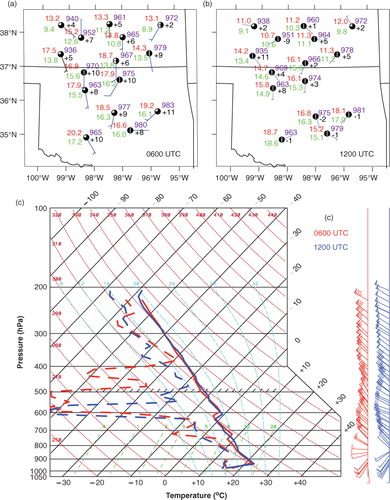
Figure 2 shows assimilated surface (top) and rawinsonde (bottom) measurements at 0600 and 1200 UTC 27 May 2001. The surface plots follow the standard station model code, except that station-level pressure (hPa, purple) is plotted instead of sea-level pressure and relative humidity (in multiples of 12.5%) is employed as a substitute for cloud cover (shaded circle, see caption). Pressure tendency (signed, black) shows the station-level pressure change for the past 3 hours. The surface measurements indicate weak winds and a relatively dry troposphere in the early morning hours. The troposphere was especially dry in mid-levels (Fig. 2c), but this dryness is less pronounced and of reduced depth at 1200 UTC. Both profiles show pronounced inversions at low levels. Winds veer from south-westerly to north-westerly with height. North-westerly wind speeds exceeded 30 m s⁻¹ between 400 and 200 hPa. The effects of assimilating these surface/tropospheric dry-bulb and dew point temperatures, wind profiles and station pressure values are discussed in Section 4.

2.5. Observed convective events during 27–31 May 2001

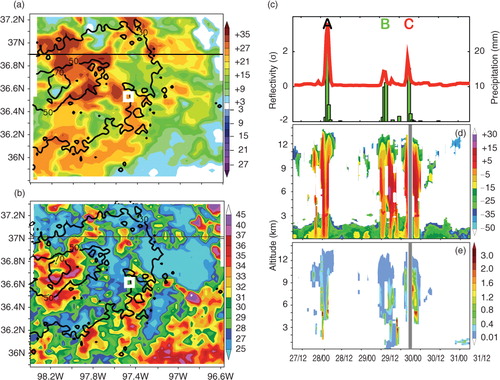
Empirical orthogonal function (EOF) analysis was applied to the observed WSR-88D radar reflectivity to provide the large-scale setting for the above convection period. EOF analysis is widely used to identify dominant patterns of variability and to reduce the dimensionality of climate data (Richman, 1986, 1987; Preisendorfer, 1988; Von Storch and Zwiers, 1999, p. 293; Wilks, 2006, p. 463). The analysis yields sets of orthogonal spatial loading patterns and their formally associated uncorrelated score time series that are widely used for comparing model simulations to observations and reanalysis (Richman, 1986; Hannachi et al., 2006). To identify the coherent spatial patterns of convection over the SGP, a correlation dispersion matrix of the WSR-88D reflectivity was used. This dispersion matrix equally weights all grid point reflectivity variability, and the resulting EOFs describe the relative variations of the spatio-temporal convection structure. The first unrotated mode (EOF1) explains 30% of the total variance of the reflectivity time series.

Inspection of the raw WSR-88D data and the EOF1 pattern extracted from them showed that three convective storms passed over the CF (Fig. 3) during 27–31 May 2001. Major convection covered the north-western two-thirds of the inner model domain, where the frequency of occurrence of WSR-88D reflectivity exceeding 10 dBZ was more than 30% (Fig. 3b). Storms with high reflectivity values were infrequent in the south-eastern portion of the domain. The peak EOF1 scores (red line, Fig. 3c) closely match the hourly precipitation rate maxima at the CF (bars, Fig. 3c). The vertical structure of the storms that passed over the CF can be seen in Fig. 3d and e, from zenith-pointing MMCR measurements and retrieved IWC and LWC obtained via Mace et al. (2006). The first storm (event A, May 27/28) was shorter-lived than the subsequent two convection events (B and C) on May 29/30, but had similarly large IWC in the middle-to-upper troposphere (5–9 km). Event A largely subsided after producing more than 25 mm h⁻¹ of precipitation at 02 UTC 28 May 2001, at which time the MMCR reflectivity was highly attenuated. In contrast, event B on 29 May 2001 had stronger reflectivity (>15 dBZ) and larger LWC in the lower troposphere. The associated precipitation was distributed over a few hours, reaching 11 mm h⁻¹ at 14 UTC. Event C started around 04 UTC 30 May 2001. It had little LWC in the lower atmosphere, but possessed significant IWC in the middle-to-upper troposphere and produced more than 15 mm precipitation in an hour at 04 UTC 30 May. These contrasting episodes provided an appropriate combination of non-precipitating and precipitating environments to evaluate the WRF-ARW model against observations.

Fig. 3 Spatial (left) and temporal (right) convection signatures over the Southern Great Plains (SGP) for 27–31 May 2001. (a) EOF1 (dimensionless) and (b) mean (shading, dBZ) and frequency (>10 dBZ, contours,%) of WSR-88D weather radar (Vance AFB, Fig. 1) reflectivity for the inner 3-km grid spaced model domain in Fig. 1 (thick broken line). (c) Time coefficients of EOF1 in (a) (standardised and scaled, red line) and hourly precipitation rates from surface meteorological observation stations (bars, mm). (d) Millimeter cloud radar reflectivity (dBZ) at the CF (located by white squares in (a), (b); from Mace et al. 2006) and (e) CF liquid (below 4 km) and ice (above 4 km) water concentration (g m⁻³) obtained via Mace et al. (2006). Letters A, B, C at top of (c) identify convective events at corresponding times (day/hour bottom abscissa). Parts of the extended low-level MMCR radar echoes below 3 km likely are contaminated by radar signals from non-cloud sources.

3. Spatial-temporal correspondence between dominant modes of simulated and observed weather radar reflectivity without DA (CNTRL)

3.1. Methods

A straightforward and comprehensive means of evaluating model performance is comparing observed and simulated radar reflectivity fields, based on mixing ratios of grid-resolved water species (Ferrier, 1994). This section summarises such comparisons for control simulations that did not involve DA (CNTRL) to permit a focus on the impact of microphysics parameterisation alone. For model verification, the observed WSR-88D Doppler radar reflectivity data were compared with simulated (column maximum) Z _es values computed using PSD specifications and mass–diameter assumptions employed in eight WRF-ARW microphysics schemes – henceforth termed Lin, WSM5, Eta, WSM6, Goddard, Thompson, WDM5 and WDM6 (Table 1) – via the full Mie calculations and accounting for atmospheric and hydrometeor attenuation.

PSD details for the eight ARW microphysics schemes are provided in Table 1, along with associated mass–size relationships or hydrometeor densities for spherical particles with constant density. In the Lin, Eta, WSM5, WSM6 and Goddard microphysics schemes, precipitating hydrometeors – rain, snow and graupel for all schemes except WSM5 and Eta (rain and snow only) – are assumed to have exponential PSDs. With the few exceptions described below, the intercept parameter of the exponential distribution N _ox is specified and the slope of the distribution is appropriately determined by assuming spherical precipitating condensates with constant density.

In WDM5 and WDM6, cloud water and rain are assumed to have generalised gamma distributions with specified shape and dispersion parameters (Lim and Hong, 2010). The number concentrations for these two hydrometeors are predicted. For all WSM/WDM schemes, the intercept for snow was assumed to be temperature dependent and the ice crystal number concentrations and mass–diameter relationships ensured ice crystal size consistency between sedimentation and ice microphysical processes (Hong et al., 2004, 2006).

Although the Eta scheme assumes exponential size distributions for rain and precipitating ice/snow, the intercept parameter for rain and the mean diameter (and hence slope parameter) for precipitating ice are retrieved from lookup tables (ETAMPNEW_DATA file). For rain, the intercept parameter depends on the rain content. For precipitating ice, the particle mean diameter and mass–density relationships (based on Houze et al., 1979) are read in during the reflectivity computations.

The Thompson scheme by default uses exponential size distributions for rain, graupel and cloud ice, but it predicts the total number concentrations of rain and ice condensates. For snow, the scheme uses a combination of exponential and gamma distributions to account for the observed super-exponential distribution of small particles and the general slope of large particles, and employs a non-spherical mass–diameter relationship m(D)=0.069 D ². The cloud water treatment applies a generalised gamma distribution, with its shape parameter being diagnosed from a specified cloud water concentration (Thompson et al., 2008).

3.2. Results

Unrotated EOF analyses of the observed and simulated Z _es fields are shown in Fig. 4, where the spatial patterns for the eight WRF-ARW microphysics simulations are computed according to their respective PSD characteristics given in Table 1. The lowest Z _es value specified was −35 dBZ. Unlike the observations (Fig. 3a), the simulated Z _es fields in Fig. 4 (columns 1 and 3) showed a more coherent convection structure across the south-western part of the inner model domain. Although there are some large discrepancies in the coherent spatial signals between the observed and simulated reflectivity values, nearly all the simulations exhibited coherent reflectivity signals west of the CF that are more consistent with the observations. EOF1 for all simulations explained 18–21% of their respective total variances, fractions that are less than the 30% variance explained by EOF1 of the observed WSR-88D data. Also, the frequency of simulated Z _es exceeding 10 dBZ was largely limited to 10–15% for most microphysics schemes. In contrast to the observations, these microphysics simulations produced more frequent severe storms east of the CF.

Fig. 4 Spatial (shading) and corresponding temporal (time series) characteristics of simulated weather radar reflectivity fields over the Southern Great Plains (SGP) for the inner 3-km grid spaced model domain (Fig. 1, thick broken line) for eight WRF microphysics experiments with no data assimilation (DA) (CNTRL) for 27–31 May 2001. Columns 1 and 3 contain EOF1 patterns (dimensionless, colour shading, arbitrary scale at bottom) and frequency of intensity (above 10 dBZ, black contours,%) of simulated reflectivity for the microphysics-based PSD simulations (Table 1). Columns 2 and 4 contain time series of scores (blue) corresponding to the EOF1 patterns in columns 1 and 3, respectively. For columns 2 and 4, the colour coding for the above time series appears at the top, along with that for a counterpart time series for EOF1 of the WSR-88D reflectivity observations (red) derived from Fig. 3a and c. All EOF time series are standardised (σ in units of mm⁶ m⁻³) and scaled by 100. Black squares in columns 1 and 3 show location of SGP Central Facility (CF).

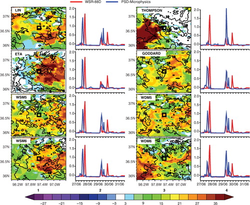
The overall differences between observed and simulated Z _es fields can more clearly be seen in the EOF score time series plots in Fig. 4 (columns 2 and 4). These plots present the EOF1 time series for the WSR-88D observations (red) and eight CNTRL microphysics simulations for which Z _es (blue) was computed using the eight WRF PSD specifications (Table 1). The most conspicuous difference between the observed and simulated reflectivity values is the time of convection onset (Fig. 4). While the WSR-88D radar showed significant reflectivity coinciding with the CF torrential precipitation on 28 May 2001 (event A), all simulated reflectivity fields exhibited their major convection 6 hours earlier on 28 May 2001. Also, absent in all simulated reflectivity EOF1 time series is the observed third convection event (C) on 30 May 2001 (Fig. 4), when large precipitation was recorded at the CF (Fig. 3c). However, all microphysics simulations correctly reproduced the second major convection event B more than 50 hours into the simulation.

4. Assessment of impact of DA and microphysics parameterisation on vertical structure of simulated clouds in CF vicinity

Model sensitivities were assessed further by comparing vertical profiles of simulated Ka-band equivalent radar reflectivity (Z _ek) with observed counterparts from the CF MMCR. These local-scale comparisons consider the impact of DA as well as microphysics parameterisation. The goal was to assess and quantify the effects of initial conditions and lateral boundary tendency specifications, and to identify the microphysics dependence of simulated thermodynamic and stability structures and individual hydrometeor species characteristics. Zhu et al. (2012) suggested that differences between microphysics simulations can indicate the influence of those parameterisations on simulated hydrometeor content, and hence cloud radar reflectivity. The computation of Z _ek employs the WRF-ARW microphysics PSDs (Table 1; discussed in Section 3.1). All simulated fields were interpolated vertically to match the vertical grid spacing of the observations. For ease of comparison in subsequent discussion of model simulations, the results of all microphysics and DA experiments are combined into single figures that each deal with a particular topic (Figs. (5–10)). However, this arrangement necessitates frequent cross-referencing between those figures in the following sections.

Fig. 5 Simulated cloud radar reflectivity profiles for 27–31 May 2001 (dBZ, colour scale at bottom) for eight WRF microphysics schemes for the following experiments: (a) no data assimilation (DA) (CNTRL), (b) observational nudging analysis (OBNUD), (c) three-dimensional variational DA (3DVAR) and (d) four-dimensional variational DA (4DVAR). Cloud radar reflectivity values were averaged over the 9×9 grid points nearest to the SGP CF (Fig. 1, dark dotted square). Middle row shows the MMCR-observed cloud radar reflectivity Best Estimate for the CF, with colour arrows indicating observed convective events A (black), B (green) and C (red) in Fig. 3c–e. WSM5(6) and WDM5(6) are WRF Single-Moment 5(6)-class and WRF Double-Moment 5(6)-class microphysics schemes, respectively. Parts of the extended low-level MMCR radar echoes below 3 km likely are contaminated by radar signals from non-cloud sources.

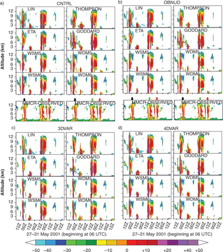
Fig. 6 Contributions (%) of individual hydrometeor species (colours, coded at top) to total simulated cloud radar reflectivity for eight WRF microphysics CNTRL simulations in Fig. 5a at five representative altitudes (1, 3, 5, 7 and 9 km) for 27–31 May 2001. Simulated cloud radar reflectivity was computed using particle size distribution (PSD) characteristics for individual microphysics schemes (Table 1), and averaged over the 9×9 grid points nearest to the SGP CF (Fig. 1, dark dotted square). For Eta microphysics, snow and ice are not differentiated. WRF single/double-moment five-category scheme (WSM5/WDM5) provides explicit treatment of cloud water, rainwater, snow and ice species. Lin, WSM6, WDM6, Goddard and Thompson microphysics schemes predict the additional graupel species. Black (A), green (B) and red (C) arrows at top indicate the three organised convective events identified in Fig. 3c–e and 5 (middle row). Finite but numerically negligible (<1e–10 kg/kg) rain mixing ratios are generated below 3 km outside the three precipitation events A, B and C in the Lin simulation, which affected the reflectivity percentage contributions when only rainwater is simulated at a given instant of time.

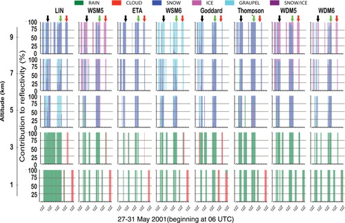
Fig. 7 Vertical profiles of correlations (values along bottom abscissa) between simulated and MMCR-observed cloud radar reflectivity for 27–31 May 2001 for eight WRF microphysics schemes for the following experiments (colour-coded at bottom): no data assimilation (DA) (CNTRL; dark blue), observational nudging analysis (OBNUD; green), three-dimensional variational DA (3DVAR; light blue) and four-dimensional variational DA (4DVAR; red). Cloud radar reflectivity values were averaged over the 9×9 grid points nearest to the SGP CF (Fig. 1, dark dotted square; Fig. 5, middle row). Black lines give vertical profiles of MMCR-observed (dashed, dBZ) and simulated (solid, dBZ) reflectivity for CNTRL experiment averaged over entire simulation period (dBZ scale is along top abscissa). Grey dotted lines provide vertical profiles of number of simulated versus MMCR-observed concurrent reflectivity pairs used in computing the correlations (count scale is along top abscissa). Colour-coded markers at the right end of each correlation profile show levels where correlations for each assimilation scheme are statistically significant at the 90% level according to a two-tailed Student's t-test (Tamhane and Dunlop, 2000, pp. 380–384). WSM5(6) and WDM5(6) are WRF Single-Moment 5(6)-class and WRF Double-Moment 5(6)-class microphysics schemes, respectively. Correlations below about 3 km are slightly affected by the presence of extended weak radar echoes outside of events A, B, C in the Mace et al.'s (2006) MMCR data.

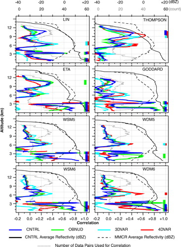
Fig. 8 Average contributions (%) of individual hydrometeor species (colours, coded at top) to total simulated cloud radar reflectivity for eight WRF microphysics schemes for CNTRL and data assimilation (DA) experiments (OBNUD, 3DVAR, 4DVAR) at five representative altitudes (1, 3, 5, 7, 9 km) for 27–31 May 2001. The overall contributions were computed by averaging hydrometeor reflectivity contributions (e.g. see Fig. 6 for CNTRL) over the simulation period. Simulated cloud radar reflectivity was computed using particle size distribution (PSD) characteristics for individual microphysics schemes (Table 1) and averaged over the 9×9 grid points nearest to the SGP CF (Fig. 1, dark dotted square). For Eta microphysics, snow and ice are not differentiated. WRF single/double-moment five-category scheme (WSM5/WDM5) provides explicit treatment of cloud water, rainwater, snow and ice species. Lin, WSM6, WDM6, Goddard and Thompson microphysics schemes predict the additional graupel species.

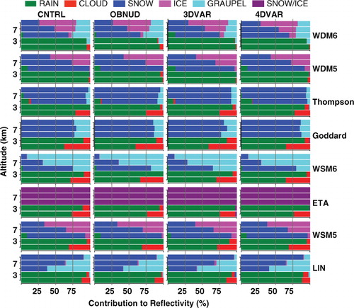
Fig. 9 Frequency bias scores (FBSs) (Section 2.3) as a function of reflectivity threshold from − 35 to + 15 dBZ at 1 dBZ intervals for eight WRF microphysics scheme simulations with (colours, defined at top) and without (CNTRL, dark lines) data assimilation (DA). Cloud radar reflectivity values were averaged over the 9×9 grid points nearest to the SGP CF (Fig. 1, dark dotted square). FBS values shown are limited to a maximum of 1.5 because of their steep increases for reflectivity thresholds exceeding + 15 dBZ. Grey-shaded envelope contains the 95% bootstrap confidence intervals (CIs) (Section 2.3) for CNTRL FBSs. Thick broken dark horizontal lines show FBS values for perfect model skill. OBNUD is surface and rawinsonde observation nudging and 3DVAR and 4DVAR are three-dimensional and four-dimensional variational DA, respectively.

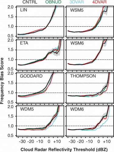
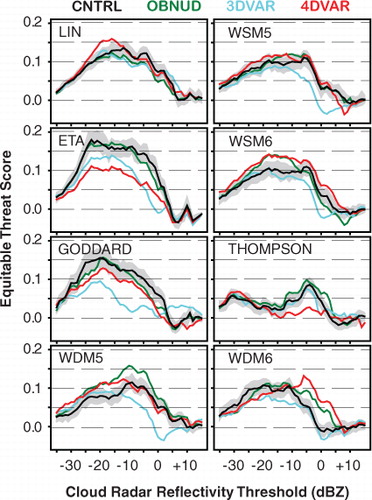
Fig. 10 Same as Fig. 9, but for equitable threat scores (ETSs) for cloud radar reflectivity thresholds between − 35 to + 15 dBZ at 1 dBZ intervals.

For each of the eight microphysics schemes, Fig. 5 compares vertical profiles of the simulated Z _ek (dBZ) for the CNTRL, OBNUD, 3DVAR and 4DVAR experiments defined in Section 2.4 for 27–31 May 2001. To facilitate comparisons, the observed MMCR reflectivity profile also is shown in Fig. 5. The contributions of individual water species to the simulated total Z _ek were assessed for each microphysics scheme by computing separately the Z _ek for cloud water, rain, snow, ice and graupel species using their appropriate PSD formulations (Table 1). The results are presented as percentages of total Z _ek at five representative altitudes (1, 3, 5, 7, and 9 km) for the CNTRL experiment (Fig. 6). The contribution of each hydrometeor species to total Z _ek was summarised further by averaging the percentage of hydrometeor contributions over the entire 27–31 May 2001 simulation period (Fig. 8). Knowledge of the percentage contribution of each hydrometeor species to total Z_ek is important to identify model deficiencies and improve the microphysical representation of clouds. However, because there are no observational data to evaluate the habits of ice-phase hydrometeors, the reflectivity contributions of frozen condensates to the total reflectivity primarily depend on each scheme's partitioning of ice-phase hydrometeors.

4.1. Simulations without DA (CNTRL)

The first well-organised storm corresponding to the highest observed surface precipitation rate – event A in Fig. 3c–e, documented observationally in the middle row of Fig. 5 – began about 2100 UTC 27 May 2001. Despite some small differences in timing, similar tropospheric cloud reflectivity was simulated for all microphysics schemes (Fig. 5a). For the Lin scheme, snow was the primary contributor to the simulated mid-to-upper tropospheric Z _ek at 0200 UTC 28 May. Also for this scheme, increased cloud water due to condensation produced extended simulated lower-tropospheric Z _ek during 1000–1400 UTC 28 May, with rainwater maximising near 2 km AGL at 1200 UTC (Figs. 5a and 6).

The second well-organised convective event (B, Figs. 3c–e and 5 middle row) occurred between 1200 and 1800 UTC 29 May 2001. Its successful simulation (Fig. 5a) involved the largest production of graupel/snow for the Lin and WSM6 schemes, and snow for Goddard, Thompson and WDM schemes (Fig. 6). For event B, Z _ek values are slightly weaker than MMCR-observed middle- and upper-tropospheric values, and stronger in the lower troposphere. Although delayed by a few hours, the vertical simulated convection profiles (Fig. 5a reflectivity profiles) compared well with the observations (Figs. 3 and 4 time series) for 1200–2100 UTC 29 May 2001.

Following event B, the model performance deteriorates appreciably (Fig. 5a, middle row). Common to all microphysics runs after the second convection event is the production of large descending motion at upper-tropospheric levels and significant (2–4 K) surface-to-mid-tropospheric cooling and upper-tropospheric warming between 0300 and 1200 UTC 30 May 2001 (not shown). As a result of these convection inhibiting factors, the model failed to produce the well-organised and extended convective storm with+15 dBZ maximum reflectivity observed by the MMCR on 30 May 2001.

The correlation between simulated and observed Z _ek is similar, with the largest correlations below 3 km for most microphysics schemes (Fig. 7), where correlations are statistically significant at the 1% level for a two-tailed Student's t-test for six of the eight schemes. The Thompson scheme attains maximum correlations in the upper troposphere because (similar to the MMCR-observed values) the simulated cloud radar reflectivities are weaker in that layer. However, the low Thompson correlations near the ground partly result from extended low-level clouds following event A, and also to this scheme's slightly delayed convection for event B. Lower-tropospheric correlations are slightly affected by the presence of extended weak radar echoes in the Mace et al.'s (2006) MMCR data. For example, when only reflectivity values exceeding −30 dBZ were used CNTRL correlations for the Lin scheme noticeably increased but they remain unchanged or increased slightly for all other microphysics schemes. However, the degree of freedom decreased considerably, which reduced the statistical significance of the correlations.

Analysis of contributions of individual hydrometeor species to total Z _ek (Fig. 8) indicates that for CNTRL, total Z _ek predominantly was produced by rainwater in the lower troposphere (<3 km) for all schemes (63–100%). The second largest contributor at low levels was cloud water, accounting for 37% of the total Z _ek at 1 km for the Goddard scheme. Large graupel contributions to reflectivity occurred in the mid troposphere (5 km) for the Lin scheme and in the upper troposphere for the WSM6 and WDM6 schemes (9 km). Despite their large graupel productions, the WSM6 and Goddard schemes melt graupel instantly around 0°C. For the five-category WSM/WDM schemes, ice contributed over 57% of the simulated reflectivity at 9 km, while the WDM6 ice contributed the largest percentages to simulated reflectivity compared to the other six-category schemes. Of the eight microphysics schemes, the Thompson scheme generated the most mid- and upper-tropospheric snow due to its regular conversion to snow of cloud ice with diameter >125 µm and also by the smaller fall speeds of snow in the scheme (e.g. Zhu et al., 2012), while the WSM/WDM five-category schemes produced the most cloud ice due to a larger (more demanding) ice-diameter threshold (500 µm) for autoconversion to snow.

This production of maximum upper-tropospheric ice, which contributed significantly to the total simulated Z _ek, was unique to five-category WSM/WDM schemes, which differ from their six-category counterparts by the presence of graupel. The faster sedimentation of graupel in the six-category schemes enhances accretion of other hydrometeors (accretion is the main process for sub-freezing graupel formation) as graupel is carried to lower levels more rapidly, and thus can result in ice hydrometeor reduction aloft (Hong et al., 2009). Hong et al. (2004) also noted that in all WSM/WDM schemes, more ice is initiated at temperatures greater than −38°C compared to Fletcher's (1962) formula used in the Lin scheme. All WSM/WDM schemes also have separate treatments for ice nuclei number concentration (determines maximum ice crystal mass that can be initiated given sufficient ice supersaturation) and ice crystal number concentration (derived as function of cloud ice mixing ratio). In contrast, the Lin microphysics scheme follows Rutledge and Hobbs (1983) for ice nuclei number concentrations (Table 1), which results in the immediate removal of supersaturation for temperatures below −43°C (Hong et al., 2004).

The FBS values in Fig. 9 for CNTRL show that many of the simulations underestimate the observations at Z _ek thresholds lower than about 0 dBZ because of their negative upper- and lower-tropospheric bias. For reflectivity thresholds larger than 0 dBZ, the Eta and Thompson schemes generally underestimate cloud reflectivity above 5 km (provided as supplemental material), while all schemes significantly overestimate the observations in the lower troposphere. The overestimation increases steeply for reflectivity thresholds above 10 dBZ for most schemes, mainly due to a large positive lower-troposphere bias. Thus, the WRF-ARW model performs better in simulating low–to-medium reflectivity values less than about 0 dBZ, for which FBS values generally are 1.0±0.3. For the Goddard, Thompson, WDM5 and WDM6 microphysics schemes, FBS values remain close to 1.0±0.2 for most threshold values below −5 dBZ. Note that the FBSs are well within the 95% CIs for all thresholds because of large sample sizes.

The ETS values are low and largely remain below 0.15 (Fig. 10, CNTRL). All microphysics simulations have low skill in reproducing the observed reflectivity at both the low and high exceedance thresholds, for which ETS values are close to 0. The largest ETS values are for thresholds between −20 and −5 dBZ. The Thompson scheme has the lowest ETS, while the Lin, Eta and Goddard schemes achieve larger ETSs for a broader range of reflectivity thresholds. Similar to the FBS values, the ETS estimates fall within the 95% CIs. The overestimation of model-simulated cloud radar reflectivity is confirmed from the ME analyses (Table 2). Inspection of the vertical profiles of ME and RMSE (see supplemental material) reveals that both errors decrease with height, indicating a generally better WRF-ARW performance in the middle and upper troposphere. Overall RMSE values (Table 2) are highest for the Lin microphysics scheme because of occasional stronger than observed simulated reflectivities in the lower troposphere during convective events A and B. Although not as large, the other schemes also have high RMSE values because of the more intense lower-tropospheric Z _ek values. In contrast, the MMCR-observed reflectivity exceeded 15 dBZ only in the middle troposphere.

4.2. Comparison of DA simulations with CNTRL simulations

The DA techniques used were discussed generally in Section 2.4. For the OBNUD simulations, model temperature, wind and water vapour mixing ratio values were nudged locally towards the 15-hourly SGP surface observations and single CF 6-hourly rawinsonde sounding between 0600 and 1200 UTC 27 May 2001. In the 3DVAR experiments, hourly SGP surface and rawinsonde observations at 0600 UTC were assimilated between 0300 and 0900 UTC 27 May 2001. For 4DVAR, hourly surface and 6-hourly rawinsonde observations were assimilated for 0600–1200 UTC 27 May 2001.

The effects of the OBNUD simulations were more pronounced in the lower-to-mid troposphere 4–5 hours after DA (Fig. 5a and b). The most coherent reflectivity increase over CNTRL was for the Lin scheme, where 5–10 dBZ increases occurred in the 1–4 km layer during 1500–1600 UTC 27 May. However, compared to CNTRL the change is most reflected in the following: increased lower- (upper) tropospheric correlations for the Lin, Goddard and WDM (Eta) schemes (Fig. 7); improved FBSs for the Eta scheme for low reflectivity threshold values (Fig. 9); higher ETSs for the WSM6, WDM5, Thompson and WDM6 schemes for several reflectivity thresholds (Fig. 10); and reduced MEs for the Goddard and Thompson schemes and RMSEs for the Thompson scheme for any verification period (Table 2). Mid-tropospheric grapuel production increased (decreased) for the Thompson (WSM6) scheme. The WSM6 and Goddard schemes continued to show graupel melting instantaneously near 0°C (Fig. 8).

The 3DVAR experiments had reduced reflectivity versus CNTRL in the first 6 hours of the simulations for many microphysics schemes (Fig. 5a and c). This reduction continued for most 3DVAR simulations during the early hours of convective event A (Fig. 5, middle row, black arrow), but the vertical and temporal extent of Z _ek showed large increases beginning 0100 UTC 28 May 2001. These reflectivity increases were associated with enhanced production of rain below 3 km and graupel and snow between 5 and 7 km. Compared to CNTRL, 3DVAR correlations were improved in the middle and upper troposphere for most microphysics schemes (Fig. 7). The 3DVAR FBSs (Fig. 9) improved over CNTRL for most microphysics simulations for large Z _ek thresholds, but they are worse than CNTRL for Z _ek<0 dBZ thresholds. Similarly, the ETSs are lower than CNTRL for nearly all Z _ek thresholds and microphysics schemes (Fig. 10). Except for the WSM5 scheme, RMSEs and MEs are lowest for most 3DVAR simulations. Although higher than those for the entire verification period, the 3DVAR MEs and RMSEs are significantly improved for the initial 36 hours of the DA for all schemes (Table 2).

The 4DVAR experiments had larger impacts on simulated reflectivities and overall model statistics than the OBNUD experiments (Fig. 5a–d). Compared to CNTRL, 4DVAR correlations are improved in the middle and upper troposphere for many microphysics schemes, but largely are weakened in the lower troposphere (Fig. 7). 4DVAR ETSs are also significantly improved for WSM5 and WSM6, but degraded for the Eta, Goddard and Thompson schemes (Fig. 10). Compared to CNTRL and OBNUD simulations, the 4DVAR experiments achieved lower RMSEs and MEs for all microphysics schemes except the WSM5 scheme (Table 2). These 4DVAR improvements are examined further in the next section.

4.3. Diagnosis of cloud and convection fields

4.3.1. Methods.

To assess further the WRF-ARW model performance for this warm-season heavy precipitation episode, observed and simulated cloud and convection characteristics in the CF vicinity were diagnosed normal to a storm-line identified for convective event A (May 27/28; Figs. 3c–e and 5 middle row, 6, 11 top two right panels), using axes of maximum water vapour mixing ratio. Event A was chosen because both rawinsonde and MMCR data were available at a time of moderate convection (prior to the maximum 26 mm h⁻¹ precipitation rate) when the MMCR signal was not attenuated completely. Additional motivation was to understand why the model produced substantially weaker Z _ek than the observed convection for event A noted in Sections 3.2 and 4.1. The analysis assumes that clouds grow in regions of highest water vapour content (e.g. Khairoutdinov and Randall, 2006), and uses 3-hourly (2300 UTC 27 May-0100 UTC 28 May 2001) mixing ratio averages for each microphysics scheme obtained via several steps.

First, for the level of maximum observed Z _ek (5.5 km AGL), the grid point with the highest mixing ratio was identified for each south-to-north grid number and those grid points were straight line fitted by least-squares linear regression. Then, to assess across-storm-line characteristics, a line perpendicular to the regression line was calculated and translated south–north/west–east to pass through the CF. The resulting axis for the CNTRL simulation for each microphysics scheme appears in all panels of Fig. 11. There is consistency between the CNTRL across-storm-line axes and their 4DVAR counterparts (not shown), and among the orthogonal maximum mixing ratio plumes from which they are derived (Fig. 11, lower left). Also, computed CNTRL Z _ek values at 5.5 km AGL (not shown) have the same northwest–southeast orientation as the water vapour maxima. Finally, for individual microphysics schemes, simulated convection and reflectivity variables were averaged over a 27 km-wide swath of 3-km spaced grid points normal to its regression axis, and vertical profiles were plotted against west-to-east grid numbers in key subsequent figures (Figs. 13 and 15). This objective determination of storm orientation allowed consistent comparisons of the vertical structures of simulated cloud characteristics. In that respect, while Fig. 11 (right, middle) shows that the across-storm-line axes align approximately along the forward edge of the squall-line southwest of the CF, more importantly they are normal to the northwest–southeast-oriented cloud streaks that passed through the CF.

Fig. 11 Simulated water vapour and observed cloud reflectivity information for convective event A (2300 UTC 27 May–0100 UTC 28 May, 2001). Left panels enclose inner-nested model domain (Fig. 1) within which coloured straight lines (coded at top right) locate across-storm-line axes for eight CNTRL [without data assimilation (DA)] microphysics simulations, constructed as described in Section 4.3. Contours in left panels give simulated mixing ratio distribution (g kg⁻¹) for a representative microphysics scheme (Lin, top left) and selected large mixing ratios for all eight CNTRL microphysics schemes (bottom left, colour coded at top right) at level of maximum observed CF MMCR reflectivity (5.5 km AGL). Crosses in left panels locate CF. Right panels present hourly sequence of WSR-88D Level III reflectivity fields (lowest elevation angle) from Vance AFB radar (Fig. 1), and the locations of the inner-nested model domain and its simulated across-storm-line axes, above. Black arrows in top two right panels identify the line storm investigated.

The variables analysed in the resulting cross-sections (Figs. 13 and 15) and related displays (Figs. 12 and 14 and 16) include Z _ek (dBZ), equivalent potential temperature (θ _e; K), convective available potential energy (CAPE; J kg⁻¹), convective inhibition energy (CIN; J kg⁻¹), relative humidity (RH;%), buoyancy (B; m s⁻²), moist static energy , and saturated moist static energy . Here, the energy terms have their standard definitions and h and h _s are expressed in K after dividing by the specific heat for air. Buoyancy is , where θ is the potential temperature and overbars can denote either temporal or spatial averages, and liquid and solid water content are neglected to allow comparison with observations (e.g. Bryan and Morrison, 2012). As there was only a single CF rawinsonde observation site for vertical profile comparisons, deviations of simulated h/h _s and B are calculated first from time-averaged CF reference profiles. To account for the diurnal cycle, those reference profiles were constructed from data averaged for the same hour of each day (e.g. 0000 UTC). Then, additionally, spatially averaged simulated reference profiles were constructed for each hour during 2300 UTC 27 May–0100 UTC 28 May 2001 by averaging parameters of interest over the 35×35 grid-point nested domain delineated in Fig. 1.

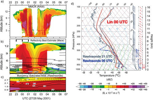
Fig. 12 Vertical structure of observed convection characteristics in the vicinity of the CF for 2100 UTC 27 May–0700 UTC 28 May 2001. (a) Time–height section of MMCR-observed raw reflectivity (with clutter removed, colour scale at bottom right), showing complete attenuation at time of maximum convection. (b) Same section for MMCR-observed reflectivity best estimate (Mace et al., 2006, colour scale at bottom right) and equivalent potential temperature from CF rawinsonde (black contours, K). In (b), arrows at top indicate times of data used for simulation result averaging in Figs. (13–16), and thick black dashed line is the 0°C isotherm. (c) Rawinsonde-based saturated moist static energy deviations (, contours, K) and buoyancy perturbations (B, shading, scale at bottom right) for the lowest 3 km. (d) Skew T–log p diagram comparing CF rawinsonde observations (blue and grey curves) and a representative CNTRL simulation (Lin microphysics, red curves) averaged over the 9×9 grid points nearest to the CF (Fig. 1, dark dotted square) for 0000 UTC 28 May 2001. Red broken line in (d) indicates surface-500 m layer CAPE. Rawinsonde launch times nearest to and within 2100 UTC 27 May–0700 UTC 28 May period were 2030, 2330, 0530 UTC. Parts of the extended low-level MMCR radar echoes below 3 km in (b) likely are contaminated by radar signals from non-cloud sources.

4.3.2. Comparison of CNTRL and 4DVAR simulations.

Figure 12 shows key observed convection characteristics during event A (Figs. 3c–e and 5 middle row, 6). The focus here is the less-MMCR-attenuating convection coinciding with the rawinsonde observation at 0000 UTC 28 May, prior to the observed heavy precipitation that caused complete MMCR attenuation at 0200 UTC 28 May 2001 (Fig. 12a). The observed convection at 0000 UTC occurred in association with high θ _e (~342 K) between 1 and 2 km (Fig. 12b), a layer with large positive B and h _s perturbations (Fig. 12c). Compared to the observations at 2100 UTC 27 May, the environment at 0000 UTC 28 May was more moist (dry) between 850 and 500 (500–400) hPa (Fig. 12d). The 0000 UTC veering of the wind with height in the lower troposphere indicates warm advection. A shallow inversion caps a 500 m-deep surface layer of nearly adiabatic lapse rate. The (partial) CAPE for a 500 m-deep near-surface air parcel was only 300 J kg⁻¹, because the 0000 UTC sounding was truncated at 415 hPa. This rawinsonde-observed temperature profile and CAPE are similar to CNTRL simulation counterparts (e.g. Fig. 12d). However, the simulated moisture was too dry (moist) between 1 and 4 (5–6) km.

Vertical cross sections along the axes in Fig. 11 are presented in Fig. 13 for Z _ek, θ _e, and h _s and B perturbations for CNTRL simulations for the eight microphysics schemes at 0000 UTC 28 May 2001. Although all CNTRL microphysics simulations produced some reflectivities in the CF vicinity (delimited by red lines between the rows in Fig. 13), only the Lin and Thompson simulations showed vertically extended Z _ek values across the entire west-to-east extent of that domain. For all CNTRL simulations, the simulated convection is associated with high θ _e and positively buoyant air southwest of the CF, where perturbations of B (from area average-reference profiles) and h_s (from time average-reference profiles) are large. Although slightly deeper, the negative simulated h _s perturbations (−5 K) near the surface are not significantly different from the observed −4 K h_s values (Fig. 12). However, the maximum simulated θ _e (~336 K) values between 1 and 2 km are lower than the observed 342 K θ _e value. Comparison shows that the Thompson and to a lesser extent Lin simulations have large B and h _s values ahead of the storm (southwest of the CF), which supported the vertically extended simulated cloud structure in the CF vicinity. The addition of graupel in the six-category WSM/WDM schemes compared to five-category non-graupel counterparts resulted in enhanced reflectivity in the lower troposphere, which underlines the importance of including graupel in reflectivity simulations. Comparison of hydrometeor profiles for the five- and six-category schemes indicated that more rainwater developed below the melting level when graupel was included as additional water species.

Fig. 13 Vertical structure of simulated convection characteristics along axes in Fig. 11 for eight CNTRL (without data assimilation [DA]) microphysics simulations averaged over 3-hourly time-steps centred on 0000 UTC 28 May 2001. Top and third rows contain horizontal-height cross-sections of Ka-band cloud radar reflectivity (shading, dBZ, colour coded at bottom) and equivalent potential temperature (contours, K), where thin black broken lines are 0°C isotherms. Second and fourth rows have same sections for lowest 3 km for perturbations of moist static energy (, contours, K) and buoyancy (B, shading, colour coded at bottom), computed as described in Section 4.3. For each microphysics scheme, all variables were averaged over 27 km normal to its axis in Fig. 11 (see Section 4.3). Thick horizontal red lines between panels indicate west-to-east extent of the Central Facility (CF) vicinity enclosed by dark dotted square in Fig. 1. The CF location is indicated by red arrows at bottom.

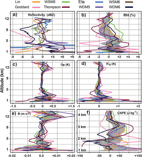
Similarities and differences between simulated and observed cloud characteristics at 0000 UTC 28 May are illustrated further in Fig. 14. All variables are averaged across the west–east extent of the CF vicinity. Variations in microphysics simulated stability parameters are shown by the 95% CIs from the mean of the eight microphysics schemes. Except for the Eta simulation, all CNTRL Z _ek values are closer to the observed Z _ek value (red line) at mid-levels. Below 3 km, the Z _ek profile for the Thompson microphysics scheme compares well with observations. While there is an overall similarity in moisture and stability profiles between the microphysics simulations and observations, the simulated relative humidity, CAPE, θ _e, B and h _s values are lower than observed counterparts between 1 and 4 km. However, there are relatively large simulated CIN values (50–200 J kg⁻¹) below 2 km, which would require large updrafts to lift boundary layer air to the level of free convection (e.g. Trier et al., 2006). Thus, compared to observations, the model developed a more stable environment and less buoyant air prior to the observed heavy convection event. The absence of the observed mid-tropospheric dry air additionally prevented the model from developing potential (convective) instability that accompanies a sharp decrease of moisture with height.

Fig. 14 Comparison of CNTRL (without data assimilation [DA]) WRF-ARW microphysics-simulated versus MMCR/rawinsonde-observed vertical profiles of cloud and atmospheric properties in CF vicinity for 2300 UTC 27 May–0600 UTC 28 May 2001. MMCR (rawinsonde) observations are instantaneous 0000 (0000 and 0600) UTC measurements at CF. All simulated values are 3-hourly averages (2300, 0000, 0100 UTC) for 9×9 grid points surrounding CF (Fig. 1). (a) MMCR-observed (red line) and simulated (other colours, coded at top) Ka-band cloud radar reflectivity. (b)–(e) Relative humidity (RH), CAPE, CIN and equivalent potential temperature (θ _e) from rawinsonde observations (red, solid is 0000 UTC, broken is 0600 UTC) and simulations (other colours, coded at top). (f)–(h) Buoyancy (B), perturbation equivalent potential temperature () and perturbation saturated moist static energy () relative to time-averaged reference profiles (see Section 4.3) for rawinsonde observations (red, solid is 0000 UTC, broken is for 0600 UTC) and simulations (other colours, coded at top). Blue lines in (f)–(h) are corresponding perturbation values, but averaged for all eight microphysics simulations and computed relative to area-averaged (35×35 grid points, Fig. 1) reference profiles (see Section 4.3). Grey envelopes in (b)–(h) span the 95% two-sided confidence intervals (CIs) (t-interval; Tamhane and Dunlop, 2000, pp. 249–250) for the average of the eight microphysics CNTRL values.

In addition to the above simulated more stable and less buoyant lower-tropospheric conditions that contributed to model departures from observed convection noted in Sections 3.2 and 4.1, all CNTRL simulations produced high dew point depressions (i.e. T−T _d) between 870 and 800 hPa for 0000–0200 UTC 28 May 2001 (not shown). For example, for the 870–800 hPa layer and 9×9 grid points surrounding the CF, the modal (most frequent) dew point depressions at 0000 UTC 28 May ranged from 6°C for the Goddard scheme to 10°C for the six-category WRF single- and double-moment schemes. These large simulated dew point depressions are associated with drying and warming above the PBL that likely is due to weaker mixing. These simulated values, which persisted for the duration of event A, were substantially higher than the observed 870–800 hPa layer modal dew point depression of less than 1°C. This poor simulation of lower-tropospheric moisture and stability characteristics appears to be the primary reason for the substantially weaker than observed Z _ek for event A, as noted in Sections 3.2 and 4.1. Also many of the precipitation efficient microphysics schemes, notably the Lin and WSM6 schemes have depleted too much water vapour from the atmosphere during the maximum model convection prior to 00 UTC 28 May 2001, which partially led to substantially weaker than observed Z _ek for event A. Simulated temperature and moisture profiles for the Thompson scheme are closer to the observations compared to the other schemes.

Compared to CNTRL, the use of 4DVAR improved Z _ek over the CF, especially for the Lin and Goddard simulations (Figs. (13–16)). The Z _ek profile improvements are associated with higher simulated values of θ _e, RH, B, h _s, and CAPE in the lowest 3 km (Figs. 15 and 16) and, in particular, the increased buoyancy ahead of the cloud structure (southwest of the CF) enhancing new storm development (Fig. 15). Although 4DVAR reduced θ _e values for the Thompson microphysics simulation and weakened the intensity of simulated Z _ek southwest of the CF vicinity, it increased Z _ek and θ _e at the leading edge near the CF (Figs. 13 and 15). In general, compared to CNTRL the increased simulated Z _ek is accompanied by enhanced tropospheric RH (Fig. 16b) and larger θ _e and CAPE values in the lower troposphere (Fig. 16c and f). Also, relative to CNTRL, 4DVAR increased (decreased) dew point temperatures in the lower (middle) troposphere during event A, the changes being largest at 0200 UTC 28 May 2001 (not shown).

Fig. 15 Same as Fig. 13 except for 4DVAR simulations. The cross-sections for each microphysics simulation are constructed along the same horizontal axis as was obtained and used for the corresponding CNTRL (without data assimilation [DA]) simulation (Fig. 11). See Section 4.3 for further explanation and justification.

Fig. 16 Comparison of 4DVAR microphysics-simulated vertical profiles of cloud and atmospheric properties in CF vicinity with counterpart CNTRL simulations (Fig. 14) for 2300 UTC 27 May–0100 UTC 28 May 2001. All simulated values are 3-hourly averages (2300, 0000, 0100 UTC) for 9×9 grid points surrounding CF (Fig. 1). 4DVAR-minus-CNTRL simulation differences (microphysics scheme colour coded at top) of (a) K_a-band cloud radar reflectivity (dBZ differences), (b) relative humidity (RH), (c) equivalent potential temperature (θ _e), (d) perturbation saturated moist static energy (), (e) buoyancy (B) and (f) CAPE. Perturbations (, B) are from time-averaged simulation reference profiles as described in Section 4.3. Grey envelopes in (b)–(f) span the 95% two-sided confidence intervals (CIs) (t-interval; Tamhane and Dunlop, 2000, pp. 249–250) for the average of the eight microphysics 4DVAR-minus-CNTRL values.

The WDM5/WDM6 simulations produced lower Z _ek than WSM5/WSM6 for both CNTRL and 4DVAR (Figs. 13 and 15). This decrease of lower-tropospheric cloud and precipitation in a stratiform region for the WDM compared to WSM simulations contrasts with results from other double- and single-moment microphysics schemes used elsewhere. Morrison et al. (2009) and Bryan and Morrison (2012) showed that simulated precipitation in a stratiform region increases in a double-moment scheme compared to a single-moment scheme, because of higher evaporation of rainwater in a single-moment scheme. It was reasoned that a double-moment scheme predicts a higher rain intercept parameter in convective cores and a smaller intercept parameter in a stratiform region. For a given mixing ratio, this is associated with increased evaporation and reduced precipitation in convective cores and reduced evaporation and increased precipitation in the stratiform region. Lim and Hong (2010) argued that the absence of enhanced melting processes for snow and graupel in Morrison et al. (2009) partly explains the different responses observed for the WSM/WDM schemes.

However, the general reduction of lower-tropospheric Z _ek for WDM simulations, compared with single-moment counterparts across the entire cross sections in Figs. 13 and 15, is likely due to enhanced evaporation from excessive rain number concentration and associated large intercept parameter predicted by the schemes. For example, the rain number concentration (not shown) predicted by the WDM6 scheme is one to two orders of magnitude larger than that predicted by the Thompson scheme, which produced a smoother and vertically extended profile of Z _ek behind the leading edge of newly developed surface convection near the CF (Figs. 13 and 15).

To explain the large dew point depressions, several preliminary additional Lin microphysics-based sensitivity simulations were conducted without DA, and they also showed relatively large dew point depressions between 1 and 2 km AGL for event A. Those simulations involved refinements to the procedures described in Section 2.2: (i) a much larger horizontal domain (163×163 inner-nested grid points with 3-km horizontal grid spacing); (ii) increased vertical grid spacing (20 vertical levels below 2 km with 91 total vertical levels, but the same in all other respects as the above CNTRL Lin simulation with 41 vertical levels); and (iii) a larger entrainment rate [double the default values computed from Eq. A11 of Hong et al. (2006)], but the same configuration as the above CNTRL Lin simulation with 41 vertical levels. While the simulated dry-bulb temperature profiles are close to the observations, all these additional simulations continued to produce much drier dew point temperatures compared to rawinsonde observations (not shown). The greatest departure from the observations was for the large-domain simulation, which developed an extremely dry environment in the low and middle troposphere. While increasing the entrainment rate reduced dew point depressions above the PBL, this experiment increased near-surface dew point depressions because of an enhanced flux of dry and warm air from above the inversion layer to the surface. Thus, at least in these preliminary additional simulations, variation of domain size, vertical resolution, or entrainment rate strength did not explain fully the CNTRL simulated large dew point depressions for event A.

Furthermore, comparison of simulated wind profiles for all experiments (original plus additional) with observations near the CF indicated that the observed southerly-to-south-easterly flow below 2 km was not correctly reproduced in any simulations for short-lived event A (e.g. Fig. 12d, below 850 hPa). This deficiency affected model stability and moisture profiles in the lower troposphere, and ultimately the convective strength of event A. Also, there were noticeable differences in the vertical profiles of moisture, temperature, and wind between the rawinsonde observations and the large-scale analysis forcing field in the vicinity of the CF, which also contributed to differences between observed and simulated convection. These additional simulation results further underline that the improvements in simulated lower-tropospheric dew point temperatures (especially) and Z _ek profiles for the 4DVAR experiments discussed earlier in this section (e.g. Figs. 13–16) and in Section 4.2, result from enhancement of the initial conditions and the consistently updated lateral boundary conditions through assimilation of hourly SGP EF surface measurements and 6-hourly CF rawinsonde data.

5. Conclusions

This article has assessed the impacts of DA and cloud microphysics parameterisation on the ability of the Advanced Research Weather Research and Forecasting (WRF-ARW) model to reproduce the vertical structure and evolution of an extended sequence of warm-season convective events (27–31 May 2001) over the US SGP. Previous attention to this type of verification/physical interpretation challenge had been minimal, both for WRF-ARW or other cloud-resolving regional climate models. Here, observations from the US Department of Energy's ACRF SGP CF site provided unique high temporal resolution data to evaluate WRF-ARW model simulations of clouds. Several evaluation metrics were used to assess comprehensively the performance of eight WRF microphysics schemes and three DA techniques.

The case study period captured a sequence of three convective storms that passed over the SGP CF. The CNTRL simulations (without DA) for eight WRF microphysics schemes at 3-km horizontal grid spacing had varied success in identifying the timing, intensity and vertical structure of the observed storm details. Of the three organised convective storms (events A, B, C) observed by the SGP CF MMCR, all microphysics schemes identified the timing and vertical structure of event B successfully, as evidenced in the simulated cloud radar (i.e. MMCR equivalent) reflectivity fields (Z _ek). Except for timing (premature evolution), event A was reasonably reproduced. However, event C was poorly simulated in the above respects. Notable microphysical differences between the eight schemes include large ice production for the five-category WSM/WDM schemes, large graupel production in the upper troposphere for the WSM6 and WDM6 schemes compared to mid-tropospheric maximum graupel production for the Lin scheme, largest mid-to-upper level snow production for the Thompson and largest low-level cloud water production for the Goddard schemes, and the instant melting of graupel near 0°C for the Goddard and WSM6 schemes.

For the CNTRL experiments, no one microphysics scheme excelled in all relative measures of skill. The Lin scheme exhibited the best FBSs for very low reflectivity thresholds, but had the largest overestimation at very high threshold values in the lower troposphere. The Eta scheme had the best ETSs, but had low correlations and significantly underestimated reflectivity in the mid-troposphere for both low and high reflectivity thresholds. The Goddard scheme highly overestimated reflectivity in the middle (upper) troposphere for nearly all (high) reflectivity threshold values. Despite the Thompson scheme having the highest reflectivity correlations in the upper troposphere, it had the lowest ETSs for several reflectivity thresholds. The WDM schemes showed much-improved FBSs in the lower troposphere for nearly all thresholds in this study but, like their single-moment counterparts, they exhibited very low correlations in the upper troposphere. WDM6's improved FBSs and high correlations in the lower troposphere likely are due to its large production of liquid water just below the melting level. Disparities in the above measures of performance likely are due partly to our focus on evaluating the vertical structure of clouds, as opposed to assessing a single-dimensional variable like precipitation. Also, some of the above relative measures of skill are slightly affected below about 3 km by the presence of extended weak radar echoes outside events A, B, C in Mace et al.'s (2006) MMCR data.

The suite of DA techniques employed – which included SGP surface and rawinsonde OBNUD and three-dimensional (3DVAR) and four-dimensional (4DVAR) variational DA of the surface and rawinsonde data – produced various simulation improvements depending on the microphysics scheme. The 4DVAR simulations increased the vertical extent of Z _ek and lower-tropospheric θ _e and CAPE during event A that produced precipitation rates of more than 25 mm h⁻¹, and thus reduced the temporal discrepancy between simulated and observed convection for event A. Profiles of dew point temperatures also showed that compared to CNTRL, 4DVAR noticeably increased (slightly reduced) moisture in the lower (middle) troposphere during event A and resulted in a better agreement with the observations. Similar differences between CNTRL and 4DVAR were not observed for event B, because the event occurred long after the DA and also this relatively longer duration event was reproduced quite well by the CNTRL simulations.

Of all the DA experiments, 3DVAR had the lowest MEs and RMSEs, although both the 3DVAR and 4DVAR simulations reduced noticeably the MEs for seven of eight microphysics schemes relative to CNTRL. However, the 3DVAR ETSs were considerably lower than CNTRL counterparts. The MEs and RMSEs were relatively large for all experiments when computed for the first 36 hours of the DA simulation. Also, none of the DA improved the simulations of event C, and the large model departure from the observed Z _ek for this event possibly is due to the long simulation time involved. The relatively limited domain size also could affect model results late in the simulation, although the success of the model in producing event B more than 50 hours into the simulation is notable. An important deduction from all simulation results is that quite accurate reproductions of lower-tropospheric moisture, temperature and wind profiles are necessary for the successful application/implementation of cloud-resolving regional models to simulate deep convection. In particular, there are needs to enhance lower-tropospheric initial and boundary conditions through DA, and to improve the physical linkages between the lower and free atmosphere.

6. Acknowledgments

This research was supported by the ASR Program of the US Department of Energy (Grant DE-FG02-05ER64062), as a contribution from the Southern Great Plains Site Scientist Team. Additional funding was from the NOAA-University of Oklahoma Cooperative Agreement #NA080AR4320904. Computations were performed at the OU Supercomputing Center for Education and Research (OSCER) at The University of Oklahoma. The authors thank G. Thompson (NCAR) and an anonymous reviewer for their very detailed formal reviews of this article, which helped improve the presentation of our methodology and interpretation of some key results.

Notes

To access the supplementary material to this article, please see Supplementary files under Article Tools online.

References

- Ackerman T. , Stokes G . The atmospheric radiation measurement program. Phys. Today. 2003; 56: 38–45.
- Barker D. M. , Huang W. , Guo Y.-R. , Bourgeois A. J. , Xiao X. N . A three-dimensional variational data assimilation system for MM5: implementation and initial results. Mon. Wea. Rev. 2004; 132: 897–914.
- Bryan G. H. , Morrison H . Sensitivity of a simulated squall line to horizontal resolution and parameterization of microphysics. Mon. Wea. Rev. 2012; 140: 202–225.
- Bukovsky M. S. , Karoly D. J . Precipitation simulations using WRF as a nested regional climate model. J. Appl. Meteorol. Climatol. 2009; 48: 2152–2159.
- Chen S.-H. , Sun W.-Y . A one-dimensional time dependent cloud model. J. Meteorol. Soc. Jap. 2002; 80: 99–118.
- Clark A. J. , Gallus W. A. Jr , Weisman M. L . Neighborhood-based verification of precipitation forecasts from convection-allowing NCAR WRF model simulations and operational NAM. Weather Forecast. 2010; 25: 1495–1509.
- Clothiaux E. E. , Ackerman T. P. , Mace G. G. , Moran K. P. , Marchand R. T. , co-authors . Objective determination of cloud heights and radar reflectivities using a combination of active remote sensors at the ARM CART sites. J. Appl. Meteorol. 2000; 39: 645–665.
- Dong X. , Minnis P. , Xi B . A climatology of midlatitude continental clouds from the ARM SGP central facility: part I: low-level cloud macrophysical, microphysical, and radiative properties. J. Clim. 2005; 18: 1391–1410.
- Dudhia J . Numerical study of convection observed during the winter monsoon experiment using a mesoscale two dimensional model. J. Atmos. Sci. 1989; 46: 3077–3107.
- Efron B. , Tibshirani R. J . An Introduction to the Bootstrap.
- Ferrier B. S . A double-moment multiple-phase four-class bulk ice scheme. Part I: description. J. Atmos. Sci. 1994; 51: 249–280.
- Ferrier B. S. , Tao W.-K. , Simpson J . A double-moment multiple-phase four-class bulk ice scheme. Part II: simulations of convective storms in different large-scale environments and comparisons with other bulk parameterizations. J. Atmos. Sci. 1995; 52: 1001–1033.
- Ferrier B. S. , Jin Y. , Lin Y. , Black T. , Rogers E. , co-authors . Implementation of a new grid-scale cloud and rainfall scheme in the NCEP Eta model. Preprints. 15th Conference on Numerical Weather Prediction. 2002; Boston: American Meteorological Society. 280–283.
- Field P. R. , Hogan R. J. , Brown P. R. A. , Illingworth A. J. , Choularton T. W. , co-authors . Parameterization of ice-particle size distributions for mid-latitude stratiform cloud. Q. J. Roy. Meteorol. Soc. 2005; 131: 1997–2017.
- Fletcher N. H . The Physics of Rain Clouds.
- Gallus W. A. Jr , Bresch J. F . Comparison of impacts of WRF dynamic core, physics package, and initial conditions on warm season rainfall forecasts. Mon. Wea. Rev. 2006; 134: 2632–2641.
- Hannachi A. , Jolliffe I. T. , Stephenson D. B. , Trendafilov N . In search of simple structures in climate: simplifying EOFs. Int. J. Climatol. 2006; 26: 7–28.
- Haynes J. M. , Marchand R. T. , Luo Z. , Bodas-Salcedo A. , Stephens G. L . A multipurpose radar simulation package: QuickBeam. Bull. Am. Meteorol. Soc. 2007; 88: 1723–1727.
- Hong S.-Y. , Dudhia J. , Chen S.-H . A revised approach to ice microphysical processes for the bulk parameterization of clouds and precipitation. Mon. Wea. Rev. 2004; 132: 103–119.
- Hong S.-Y. , Lim J.-O. J . The WRF single-moment 6-class microphysics scheme (WSM6). J. Kor. Meteorol. Soc. 2006; 42: 129–151.
- Hong S.-Y. , Lim K.-S. S. , Kim J.-H. , Lim J.-O. J. , Dudhia J . Sensitivity study of cloud-resolving convective simulations with WRF using two bulk microphysical parameterizations: ice-phase microphysics versus sedimentation effects. J. Appl. Meteorol. Climatol. 2009; 48: 61–76.
- Hong S.-Y. , Noh Y. , Dudhia J . A new vertical diffusion package with an explicit treatment of entrainment processes. Mon. Wea. Rev. 2006; 134: 2318–2341.
- Houze R. A. Jr . Cloud Dynamics.
- Houze R. A. Jr , Hobbs P. V. , Herzegh P. H. , Parsons D. B . Size distributions of precipitation particles in frontal clouds. J. Atmos. Sci. 1979; 36: 156–162.
- Hu X.-M. , Nielsen-Gammon J. W. , Zhang F . Evaluation of three planetary boundary layer schemes in the WRF model. J. Appl. Meteorol. Climatol. 2010; 49: 1831–1844.
- Jankov I. , Gallus W. A. Jr , Segal M. , Koch S. E . Influence of initial conditions on the WRF-ARW model QPF response to physical parameterization changes. Weather Forecast. 2007; 22: 501–519.
- Jankov I. , Gallus W. A. Jr , Segal M. , Shaw B. , Koch S. E . The impact of different WRF model physical parameterizations and their interactions on warm season MCS rainfall. Weather Forecast. 2005; 20: 1048–1060.
- Jankov I. , Bao J.-W. , Neiman P. , Schultz P. J. , Yuan H , co-authors . Evaluation and comparison of microphysical algorithms in ARW-WRF model simulations of atmospheric river events affecting the California Coast. J. Hydrometeor. 2009; 10: 847–870.
- Kain J. S. , Fritsch J. M . Emanuel K. A. , Raymond D. J . Convective parameterization for mesoscale models: the Kain–Fritsch scheme. The Representation of Cumulus Convection in Numerical Models of the Atmosphere. 1993; Boston: American Meteorological Society. 165–170. Meteor. Monogr No. 24.
- Kain J. S. , Weiss S. J. , Levit J. J. , Baldwin M. E. , Bright D. R . Examination of convection-allowing configurations of the WRF model for the prediction of severe convective weather: the SPC/NSSL spring program 2004. Weather Forecast. 2006; 21: 167–181.
- Khairoutdinov M. , Randall D . High-resolution simulation of shallow-to-deep convection transition over land. J. Atmos. Sci. 2006; 63: 3421–3436.
- Lang S. , Tao W.-K. , Lang S. , Cifelli R. , Olson W. , Halverson J. , co-authors . Improving simulations of convective system from TRMM LBA: easterly and westerly regimes. J. Atmos. Sci. 2007; 64: 1141–1164.
- Leung L. R. , Kuo Y.-H. , Tribbia J . Research needs and directions of regional climate modeling using WRF and CCSM. Bull. Am. Meteorol. Soc. 2006; 87: 1747–1751.
- Lhermitte R . A 94-GHz Doppler radar for cloud observations. J. Atmos. Ocean. Tech. 1987; 4: 36–48.
- Lhermitte R . Attenuation and scattering of millimeter wavelength radiation by clouds and precipitation. J. Atmos. Ocean. Tech. 1990; 7: 464–479.
- Lhermitte R . Centimeter and Millimeter Wavelength Radars in Meteorology.
- Liebe H. J . An updated model for millimeter wave propagation in moist air. Radio. Sci. 1985; 20: 1069–1089.
- Lim K.-S. S. , Hong S.-Y . Development of an effective double-moment cloud microphysics scheme with prognostic cloud condensation nuclei (CCN) for weather and climate models. Mon. Wea. Rev. 2010; 138: 1587–1612.
- Lin Y.-L. , Farley R. D. , Orville H. D . Bulk parameterization of the snow field in a cloud model. J. Clim. Appl. Meteorol. 1983; 22: 1065–1092.
- Luo Y. , Krueger S. K. , Xu K.-M . Cloud properties simulated by a single-column model. Part II: evaluation of cumulus detrainment and ice-phase microphysics using a cloud-resolving model. J. Atmos. Sci. 2006; 63: 2831–2847.
- Mace G. G. , Benson S. , Sonntag K. L. , Kato S. , Min Q. , co-authors . Cloud radiative forcing at the atmospheric radiation measurement program climate research facility: 1. Technique, validation, and comparison to satellite-derived diagnostic quantities. J. Geophys. Res. 2006; 111 D11S90.
- Mlawer E. J. , Taubman S. J. , Brown P. D. , Iacono M. J. , Clough S. A . Radiative transfer for inhomogeneous atmosphere: RRTM, a validated correlated-k model for the longwave. J. Geophys. Res. 1997; 102: 16663–16682.
- Morrison H. , Grabowski W. W . Comparison of bulk and bin warm-rain microphysics models using a kinematic framework. J. Atmos. Sci. 2007; 64: 2839–2861.
- Morrison H. , Thompson G. , Tatarskii V . Impact of cloud microphysics on the development of trailing stratiform precipitation in a simulated squall line: comparison of one- and two-moment schemes. Mon. Wea. Rev. 2009; 137: 991–1007.
- Mullen S. L. , Buizza R . Quantitative precipitation forecasts over the United States by the ECMWF ensemble prediction system. Mon. Wea. Rev. 2001; 129: 638–663.
- Otkin J. A. , Greenwald T. J . Comparison of WRF model-simulated and MODIS-derived cloud data. Mon. Wea. Rev. 2008; 136: 1957–1970.
- Parrish D. F. , Derber J. C . The National meteorological center's spectral statistical interpolation analysis system. Mon. Wea. Rev. 1992; 120: 1747–1763.
- Preisendorfer R. W . Principal Component Analysis in Meteorology and Oceanography.
- Qian Y. , Ghan S. J. , Leung L. R . Downscaling hydroclimatic changes over the Western US based on CAM subgrid scheme and WRF regional climate simulations. Int. J. Climatol. 2010; 30: 675–693.
- Raghavan S . Radar Meteorology.
- Richman M. B . Rotation of principal components. Int. J. Climatol. 1986; 6: 293–335.
- Richman M. B . Rotation of principal components: a reply. Int. J. Climatol. 1987; 7: 511–520.
- Rutledge S. A. , Hobbs P. V . The mesoscale and microscale structure and organization of clouds and precipitation in midlatitude cyclones. Part VIII: a model for the “seeder-feeder” process in warm-frontal rainbands. J. Atmos. Sci. 1983; 40: 1185–1206.
- Schaefer J. T . The critical success index as an indicator of warning skill. Weather Forecast. 1990; 5: 570–575.
- Schwartz C. S. , Kain J. S. , Weiss S. J. , Xue M. , Bright D. R. , co-authors . Next-day convection-allowing WRF model guidance: a second look at 2-km versus 4-km grid spacing. Mon. Wea. Rev. 2009; 137: 3351–3372.
- Skamarock W. C. , Klemp J. B. , Dudhia J. , Gill D. O. , Barker D. M. , co-authors . A Description of the Advanced Research WRF Version 3.
- Skamarock W. C. , Klemp J. B . A time-split nonhydrostatic atmospheric model for weather research and forecasting applications. J. Comput. Phys. 2008; 227: 3465–3485.
- Stensrud D. J . Parameterization Schemes: Keys to Understanding Numerical Weather Prediction Models.
- Stokes G. M. , Schwartz S. E . The atmospheric radiation measurement (arm) program: programmatic background and design of the cloud and radiation test bed. Bull. Am. Meteorol. Soc. 1994; 75: 1201–1221.
- Tamhane A. C. , Dunlop D. D . Statistics and Data Analysis: From Elementary to Intermediate.
- Tao W.-K. , Simpson J. , Baker D. , Braun S. , Chou M.-D. and co-authors . Microphysics, radiation and surface processes in the Goddard Cumulus Ensemble (GCE) model. Meteorol. Atmos. Phys. 2003; 82: 97–137.
- Thompson G. , Field P. R. , Rasmussen R. M. , Hall W. D . Explicit forecasts of winter precipitation using an improved bulk microphysics scheme. Part II: implementation of a new snow parameterization. Mon. Wea. Rev. 2008; 136: 5095–5115.
- Trier S. B. , Davis C. A. , Ahijevych D. A. , Weisman M. L. , Bryan G. H . Mechanisms supporting long-lived episodes of propagating nocturnal convection within a 7-day WRF model simulation. J. Atmos. Sci. 2006; 63: 2437–2461.
- US Department of Energy. Atmospheric System Research (ASR) Science and Program Plan.
- Von Storch H. , Zwiers F. W . Statistical Analysis in Climate Research. 1999; Cambridge University Press, USA. 484.
- Warner T. T . Quality assurance in atmospheric modeling. Bull. Am. Meteorol. Soc. 2011; 92: 1601–1610.
- Weisman M. L. , Davis C. , Wang W. , Manning K. W. , Klemp J. B . Experiences with 0–36-h explicit convective forecasts with the WRF-ARW model. Weather Forecast. 2008; 23: 407–437.
- Wheatley D. M. , Stensrud D. J . The impact of assimilating surface pressure observations on severe weather events in a WRF mesoscale ensemble system. Mon. Wea. Rev. 2010; 138: 1673–1694.
- Wilks D. S . Statistical Methods in the Atmospheric Sciences.
- Wu X. , Park S. , Min Q . Seasonal variation of cloud systems over ARM SGP. J. Atmos. Sci. 2008; 65: 2107–2129.
- Zhang Y. , Dulière V. , Mote P. W. , Salathe E. P. Jr . Evaluation of WRF and HadRM mesoscale climate simulations over the US Pacific Northwest. J. Clim. 2009; 22: 5511–5526.
- Zhu P. , Dudhia J. , Field P. R. , Wapler K. , Fridlind A. , co-authors . A limited area model (LAM) intercomparison study of a TWP-ICE active monsoon mesoscale convective event. J. Geophys. Res. 2012; 117 D11208.