Ensemble Kalman filter assimilation of near-surface observations over complex terrain: comparison with 3DVAR for short-range forecasts

ABSTRACT

Surface observations are the main conventional observations for weather forecasts. However, in modern numerical weather prediction, the use of surface observations, especially those data over complex terrain, remains a unique challenge. There are fundamental difficulties in assimilating surface observations with three-dimensional variational data assimilation (3DVAR). In this study, a series of observing system simulation experiments is performed with the ensemble Kalman filter (EnKF), an advanced data assimilation method to compare its ability to assimilate surface observations with 3DVAR. Using the advanced research version of the Weather Research and Forecasting (WRF) model, results from the assimilation of observations at a single observation station demonstrate that the EnKF can overcome some fundamental limitations that 3DVAR has in assimilating surface observations over complex terrain. Specifically, through its flow-dependent background error term, the EnKF produces more realistic analysis increments over complex terrain in general. More comprehensive comparisons are conducted in a short-range weather forecast using a synoptic case with two severe weather systems: a frontal system over complex terrain in the western US and a low-level jet system over the Great Plains. The EnKF is better than 3DVAR for the analysis and forecast of the low-level jet system over flat terrain. However, over complex terrain, the EnKF clearly performs better than 3DVAR, because it is more capable of handling surface data in the presence of terrain misrepresentation. In addition, results also suggest that caution is needed when dealing with errors due to model terrain representation. Data rejection may cause degraded forecasts because data are sparse over complex terrain. Owing to the use of limited ensemble sizes, the EnKF analysis is sensitive to the choice of horizontal and vertical localisation scales.

• data assimilation
• ensemble Kalman filter
• 3DVAR
• complex terrain
• short-range weather forecasting
• surface observations

1. Introduction

Surface observations are important for weather forecasts, but their use in numerical weather prediction (NWP) has proven difficult. Before NWP became the key tool for operational weather prediction, surface weather maps played a dominant role in weather forecasting; forecasters routinely made predictions using the historical evolution of surface meteorological fields illustrated by a series of weather maps. With the rapid development of NWP and increased computer power during the last half century, NWP products have replaced weather maps and become the main guidance for the modern weather forecast. NWP, however, determines weather forecasts in a different way: the future atmospheric state is calculated from the current state by integrating a numerical model. In order to produce a skilful forecast from NWP, an accurate three-dimensional initial analysis is required (Gandin, 1963; Kalnay, 2003). As advanced data assimilation techniques have been developed (Daley, 1991; Lewis et al., 2006; Evensen, 2007), various types of data (including satellite data) have been assimilated into numerical models, leading to significant improvements in forecasting accuracy.

Despite these advances in data assimilation and NWP, the use of surface observations remains a challenging problem. Currently, only a limited number of surface observations are used in NWP. In the National Centres for Environmental Prediction/National Centre for Atmospheric Research (NCEP/NCAR) 50-yr reanalysis (Kalnay et al., 1996) only surface pressure observations were assimilated. In the North American Regional Reanalysis project (NARR; Mesinger et al., 2006) only surface pressure, wind at 10-m height level, and relative humidity at the 2-m level were assimilated into the model; surface temperature (usually air temperature at the 2-m height level) was found to be significantly detrimental to forecasts and was not assimilated into NARR. Similarly, no 2-m temperature data were assimilated into the model for the European Centre for Medium-Range Weather Forecasts (ECMWF) operational analysis and ECMWF 40-yr reanalysis project (ERA 40; Simmons et al., 2004). In addition, due to significant orography, surface data assimilation becomes a challenge in NWP and data assimilation applications.

Similar problems were also found in the NCEP operational regional analysis system (Rogers et al., 2005). Experiments conducted in the summer of 2003 indicated that the assimilation of surface temperature observations over land in the North American Mesoscale (NAM) model often degraded forecasts. It was determined that the Eta three-dimensional variational data assimilation (3DVAR) system, using the step mountain coordinate, had difficulty in limiting the vertical influence of surface observations. The problem remains in the latest version of the operational Non-hydrostatic Mesoscale Model (NMM) core of the Weather Research and Forecasting (WRF) model. To meet the needs of weather analysis and forecasting as well as the verification of the National Digital Forecasting Database (NDFD), a 2DVAR scheme is used to assimilate surface observations into a real-time mesoscale analysis (RTMA) system (DiMego, 2006; De Pondeca et al., 2011) at NCEP. This system is operated independently from the operational WRF model. Therefore, except for some selected Mesonet data that are assimilated into the Rapid Update Cycle (RUC; Benjamin et al., 2004) and Rapid Refresh (Benjamin et al., 2011), no Mesonet data are assimilated into other components of the operational analysis system. Meanwhile, limited attention has been given to the use of the surface observations in data assimilation and parameter estimation (Hacker and Snyder, 2005; Lee et al., 2005; Xie et al., 2005; Dong et al., 2007; Fujita et al., 2007; Hacker et al., 2007).

Specifically, considerable difficulty has been encountered when assimilating surface observations over complex terrain, as the accuracy of representation of the realistic terrain in NWP is usually limited by both the horizontal and vertical resolution of the forecast model. Because terrain data used in the model must be modified to conform to the model resolution, the variability of the terrain within each grid cell influences the overall resolved orographic and sub-grid scale processes. This causes problems in: (1) representing the orography in the dynamics and physics of the numerical model; and (2) assimilating near-surface data. The latter is referred to as a ‘misrepresentation’ problem and makes the process of quality control and the assimilation of these data complex and difficult.

These problems in near-surface data assimilation have also been well recognised for variational data assimilation methods (e.g. 3DVAR) in operational practice. During the last decade, ensemble Kalman filter (EnKF) techniques have been advanced significantly in the research community. Previous studies (e.g. Meng and Zhang, 2008a, 2008b) demonstrate that the EnKF outperforms 3DVAR. However, while all those studies integrate many types of observation in their data assimilation experiments, none emphasises the assimilation of surface observations. In addition, progress has been made in examining the impact of surface data assimilation on short-range weather forecasts. For instance, Stensrud et al. (2009) assimilated surface observations into the WRF model with an EnKF and found that the analyses reproduced the cold pools beneath the precipitation system. Ancell et al. (2011) demonstrated that the WRF EnKF surface analyses and subsequent short-term forecasts are generally better than forecasts from the NCEP Global Forecast System (GFS) and NAM. In addition, Hacker and Snyder (2005) showed that assimilation of surface observations in a one-dimensional column model resulted in error reductions throughout the boundary layer. However, in these studies, little work has been reported evaluating whether the EnKF overcomes the existing problems for 3DVAR in surface data assimilation.

In order to initiate this investigation, in this study, a series of observing system simulation experiments (OSSEs) is performed with two data assimilation methods: a 3DVAR, which is widely applied in current operational practice, and the EnKF. The purpose of the study is to examine their respective problems and advantages in assimilating near-surface observations, not only to understand the fundamental problems in assimilating surface observations with the current 3DVAR method but also to evaluate the ability of the EnKF to deal with surface observations. Specifically, we perform OSSEs with idealised settings to investigate the problems associated with the assimilation of the surface wind at the 10-m height level (10-m wind hereafter) and temperature at the 2-m height level (2-m temperature hereafter) into an advanced research version of the WRF (WRF ARW) model. With OSSEs in a short-range forecast, we can isolate various factors that affect the use of near-surface observations, thus enhancing our understanding of the major factors that could limit our ability to assimilate surface data.

The paper is organised as follows: Section 2 briefly describes the WRF model and its 3DVAR and EnKF data assimilation systems. Section 3 briefly introduces the set up of the OSSEs. Section 4 discusses the experiments using the assimilation of a single observation over both flat and complex terrain. Results from both 3DVAR and the EnKF are compared. Section 5 shows the outcomes from the assimilation of multiple observations over North America. Section 6 examines the impact of the misrepresentation of terrain in surface data assimilation. Advantages and disadvantages of 3DVAR and the EnKF are further discussed. Summary and concluding remarks are provided in Section 7.

2. Description of the WRF model and data assimilation systems

2.1. WRF model

The WRF model is a mesoscale community NWP system. It is designed to serve both operational forecasting and atmospheric research needs. The WRF model features multiple dynamic cores. This study employs the advanced research version of the WRF model (WRF ARW). The WRF ARW is based on a Eulerian solver for the fully compressible non-hydrostatic equations, is cast in flux conservation form, and uses a mass (hydrostatic pressure) vertical coordinate. The solver uses a third-order Runge-Kutta time integration scheme coupled with a split-explicit second-order time integration scheme for the acoustic and gravity-wave modes. Fifth-order upwind-biased advection operators are used in the fully conservative flux divergence integration; second- to sixth-order schemes are run-time selectable. The WRF ARW carries multiple physical options for cumulus, microphysics, planetary boundary layer (PBL), and radiation physical processes. Details of the model are provided in Skamarock et al. (2008).

2.2. WRF 3DVAR

Along with the WRF ARW, a 3DVAR system was developed based on the NCAR/Penn State University Mesoscale Model Version 5 (MM5) 3DVAR system (Barker et al., 2004a, 2004b). The 3DVAR system provides an analysis x ^a via the minimisation of a prescribed cost function J(x),1

Commonly, in eq. (1), the analysis x=x ^a represents an a posteriori maximum likelihood (minimum variance) estimate of the true state of the atmosphere given two sources of data: the background (previous forecast) x ^b and observations y ^o (Lorenc, 1986). The analysis fit to these data is weighted by estimates of their errors: B and O are the background and observational error covariance matrices, respectively; y=H(x), and H is a linear or non-linear operator used to transform the gridpoint state x to estimated observations; i denotes each type of observational data and n represents the total number of data types.

The configuration of the WRF 3DVAR system is based on a multivariate incremental formulation (Courtier et al., 1994). The preconditioned control variables are stream function, unbalanced velocity potential, unbalanced temperature, unbalanced surface pressure, and pseudo- relative humidity. With WRF 3DVAR, users have an option to generate the background error covariance term (B matrix) to achieve consistency between the background error term and the model resolution.

In this study, statistics of the differences between daily 24-hour and 12-hour forecasts valid at 0000 UTC and 1200 UTC for 1 month (June 2008) are paired (i.e. a total of 60 samples) and used to estimate background error covariance with the so-called NMC (National Meteorological Centre, now known as NCEP) method (Parrish and Derber, 1992; Wu et al., 2002; Barker et al., 2004a 2004b). Specific steps to generate the background error term include the following: (1) convert the WRF forecast variables to preconditioned control variables and then remove the mean for each variable and each model level; (2) calculate ‘unbalanced’ control variables and conduct regression analysis to determine multivariate correlations between perturbation fields; (3) project the perturbations from model levels onto a climatologically averaged (in time, longitude and latitude) eigenvector using empirical orthogonal functions (EOFs), thus obtaining the vertical component of the background error covariance; and (4) perform linear regression of the horizontal correlations to calculate recursive filter length-scale.

The background error covariance matrix (B matrix) plays an important role in a 3DVAR system. It influences the analysis fit to the observations and also defines the domain of influence of observations. Horizontally the background error correlations are assumed to be a Gaussian function:2

where r is the distance between the model grid point and the observation location; s is the length-scale of the Gaussian function that determines how far the observation information can be spread spatially. B(0) is the background error covariance at the observation location and B(r) is the background error covariance at the model grid point at a distance r away from the observation location. The observational information is spread using a recursive filter (Wu et al., 2002; Baker et al., 2004b), while the vertical relation is represented by applying the empirical orthogonal decomposition technique. Since the background error covariance in 3DVAR is generated by mean statistics, it is constant throughout the data assimilation experiment.

2.3. Ensemble Kalman filter for WRF

The EnKF is a different way of performing data assimilation. Specifically, in the 3DVAR method, the minimisation of (1) requires a prior estimate of the background error covariance B. In the EnKF, the analysis is achieved by x ^a =x ^f +K[y ^o −H(x ^f )] with a Kalman gain matrix K=P ^f H ^T (HP ^T H ^T +R)⁻¹ where P ^f is the sample background error covariance and is estimated using an ensemble of k forecasts (Evensen, 1994).3

where the overbar represents the ensemble average. As ensemble forecasts are used in generating the background error term, the background error covariance in the EnKF is flow-dependent.

Research on the EnKF started with Evensen (1994) and Houtekamer and Mitchell (1998). Their methods can be classified as the EnKF with perturbed observations. Another type of EnKF is a class of deterministic square root filters (Anderson, 2001; Bishop et al., 2001; Whitaker and Hamill, 2002), which consists of a single analysis based on the ensemble mean, and in which the analysis perturbations are obtained from the square root of the Kalman filter analysis error covariance. Tippett et al. (2003) described serial implementations of the square root filters and argued the square root filter increases efficiency by avoiding the inversion of large matrices.

A WRF ensemble data assimilation system has been developed at NCAR since 2003 (www.image.ucar.edu/DAReS/; Chen and Snyder, 2007; Anderson et al., 2009; Torn, 2010) with the WRF ARW model and the Data Assimilation Research Testbed (DART/WRF) ensemble adjustment Kalman filter (EAKF; Anderson, 2001, 2003; Anderson et al., 2009). The EAKF uses observations to update the WRF ARW model state (analysis) variables including wind components, temperature, mixing ratio of water vapour, cloud liquid water, rain, ice and snow, surface pressure, geopotential height, and column mass of dry air. The assimilation of any type of observation can produce increments for all of the analysis variables through the forecast (prior state) ensemble sample covariance (Anderson et al., 2009).

Small ensemble size and model errors affect the performance of the EnKF. Thus, localisation and covariance inflation are commonly used in many applications. Specifically, sampling errors are present due to the use of small ensemble size to reduce the computational cost. Spuriously large error covariance estimates between a state variable and a remote observation can be produced by using a small ensemble. Spatial localisation is a practical strategy that eliminates the impact of observations beyond a cut-off distance (Houtekamer and Mitchell, 1998; Hamill et al., 2001; Anderson, 2012). It has been demonstrated that localisation can mitigate the spurious correlations to some degrees (Houtekamer and Mitchell, 1998 2001; Hamill et al., 2001; Hacker et al., 2007). Covariance inflation increases the prior ensemble estimates of the state variance and can reduce the impact of model error and avoid filter divergence (Anderson, 2007; Miyoshi, 2011; Buehner, 2012). In particular, DART/WRF uses a hierarchical Bayesian approach (Anderson, 2007), in which covariance inflation values are adaptively estimated and can vary temporally and spatially.

3. Observing system simulation experiments

To simplify the complexities of near-surface data assimilation and also examine the key factors that affect it, OSSEs are used in this study, rather than real data assimilation experiments.

A time period of 0000 UTC to 1200 UTC 5 June 2008 is chosen arbitrarily for a case study. During this period, a cold front system was passing over the western US (complex terrain) and its eastern extension was a stationary front. It was moving south-eastward and its eastern part was approaching the Great Plains. Under the influence of the front, a low-level jet (LLJ) system was evolving over the Great Plains. For OSSEs, the nature run (i.e. the ‘truth’) is generated by integrating the WRF ARW model for a 12-hour period, initialised by the NCEP NAM analysis at 0000 UTC 5 June 2008. Fig. 1a shows the weather map of 0000 UTC 5 June 2008 from the nature run. The cold front and LLJ are clearly revealed at this time.

Fig. 1.  Synoptic maps at 0000 UTC 05 June 2008 for nature run (a) and control run (b). The wind barbs denote the wind fields at 50 m AGL. Shaded contour represents the wind speeds. The contours show the temperature at 700 hPa pressure level (2°C interval). The thick black line denotes the cold front. The large box denotes the key front region, that is, used for calculations in Figs. 12, 17, 19 and 20. The small box denotes the key LLJ region used for the calculation in Fig. 12.

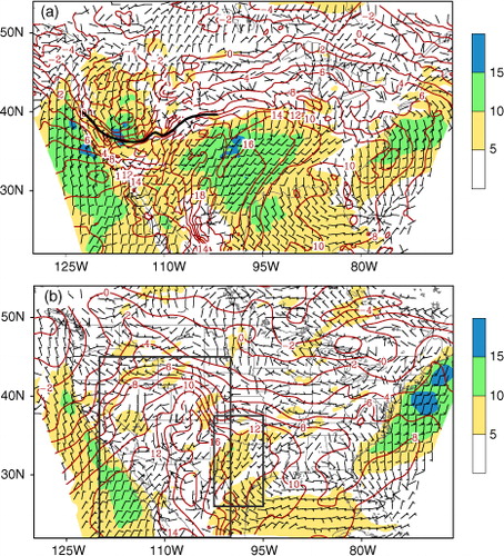
In order to account for the initial and boundary errors, the control run is randomly chosen to begin with a 6-hour forecast valid at 0000 UTC made during the first week (1–7) of June 2008 (e.g. 1 June 2008, which eliminates errors in the diurnal variation but still produce enough differences between the ‘control run’ and the ‘truth’), initialised by the NCEP GFS Final (FNL) analysis at 1×1 degree resolution. As shown in Fig. 1b, the control run completely misses the cold front and LLJ systems. The differences between the initial conditions of the ‘nature run’ and ‘control run’ are sufficient to demonstrate the effect of the data assimilation.

Considering the extent of model errors compared to the real world, different physical parameterisations are used for the nature run and control run. Specifically, model physics options used in the nature run include the Yonsei University (YSU) planetary boundary layer scheme, the thermal diffusion land surface scheme, the Lin microphysical scheme, the Kain-Fritsh cumulus parameterisation, the long-wave Rapid Radiative Transfer Model (RRTM) and the Dudhia short-wave parameterisation model (see details in Skamarock et al., 2008). In the control run, the Mellor–Yamada–Janjic (MYJ) planetary boundary layer scheme, the Noah land surface model as well as the WRF single-moment 6-class microphysics (WSM6) scheme are used while other physics are the same as those used in the nature run.

Model terrain is the same in the nature run and control run in most of the following numerical experiments except for a set of experiments discussed in Section 5 that examine the effect of the terrain misrepresentation. Model horizontal resolution (grid spacing) is set at 27 km, which includes 135 and 195 grid points in south-north and west-east direction, respectively. The model vertical structure consists of 36 η levels in a terrain-following hydrostatic-pressure coordinate with the top of the model set at 50 hPa, where η=(P _h −P _ht )/(P _hs −P _ht ). While p _h is the hydrostatic component of the pressure, p _hs and p _ht refer to pressure values along the surface and top boundaries, respectively. The η levels are placed close together in the low-levels (below 500hPa) and are relatively coarsely spaced above.

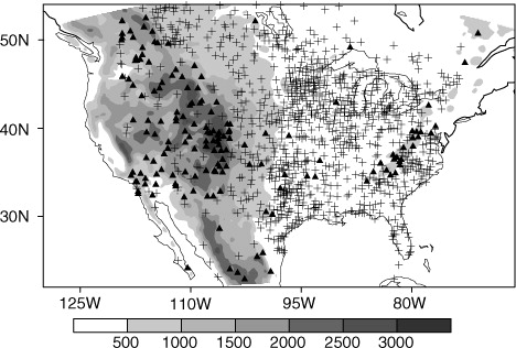
For the experiments with both the EnKF and 3DVAR, simulated hourly surface observations are generated by interpolating the nature run data to the surface station locations (as shown in Fig. 2) with unbiased random errors, which are not larger than the statistics of observational errors. Consistent with the statistics of a large sample of the data and Hacker and Snyder (2005), the observational variances are specified as 1.0 K² and 2.0 m² s⁻² for 2-m temperature and 10-m wind, respectively. For the data assimilation experiments, 2-m temperature and/or 10-m winds are assimilated into the WRF ARW model.

Fig. 2.  Distribution of surface observation stations (plus signs) and terrain heights (shaded contour; unit: m). The two solid dots denote the locations of the two stations in single station experiments.

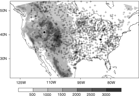
In the experiments with the EnKF, 32 ensemble members are used. Ensemble initial perturbations are obtained by so-called fixed covariance perturbations (FCPs; Torn et al., 2006) 6 hours prior to the data assimilation. In FCPs, ensemble perturbations are derived by drawing random perturbations from the 3DVAR system, which are scaled by 1.5. All members are then spun-up by running forward for 6 hours until the observations are available at the beginning of the data assimilation. Since 3DVAR experiments commonly use 6-hour forecast as a first guess for the data assimilation experiment, we choose a short ensemble spin-up period in the EnKF to ensure a fair comparison.

4. Results from assimilating observation(s) from a single station

In order to examine the influence of observations and the impact of different background terms from 3DVAR and the EnKF on surface data assimilation, experiments are first conducted by assimilating observation(s) from a single observation station. To compare the performance of 3DVAR and the EnKF over flat and complex terrain, one observation station over mountainous terrain (41.04°N, 112.98°W) and one station over flat terrain (38.0°N, 85.0°W) are selected for various experiments. All single station assimilations are conducted at 0000 UTC 5 June 2008.

4.1. 3DVAR

Figure 3 shows the 3DVAR analysis increments of temperature and u and v wind components at the lowest model level over the mountainous area by assimilating temperature only, wind (u and v components) only and both temperature and wind. Apparently, the analysis increments show mainly large-scale features and spread over the mountainous regions. Figure 4 illustrates the analysis increments over flat terrain at the lowest model level. Except for the differences in the increment shapes due to the sign of the innovation vector over the observation point (O-B), the major features of the analysis increments are similar to those over complex terrain (Fig. 3). Note that the analysis increments of u (or v) wind component from assimilating temperature only are much smaller than those from assimilating u and v components only. Therefore, Figs. 3e, 3h, 4e, and 4h are similar to 3f, 3i, 4f, and 4i, respectively.

Fig. 3.  The 3DVAR analysis increments of temperature (K; top row), u-component (m s⁻¹; middle row) and v-component (m s⁻¹; bottom row) of wind at the lowest model level with assimilation of 2-m temperature (left column), 10-m winds (middle column) and both 2-m temperature and 10-m winds (right column) from a single observation station over complex terrain. The shaded contours show the terrain heights (unit: m). ‘+' denotes the location of the observation station.

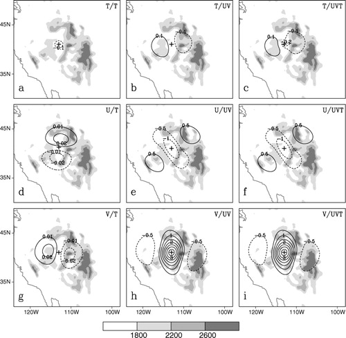
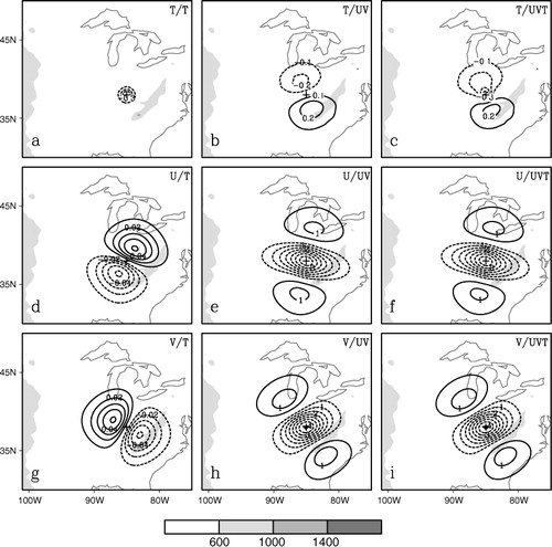
Fig. 4.  Same as Fig. 3, except over flat terrain.

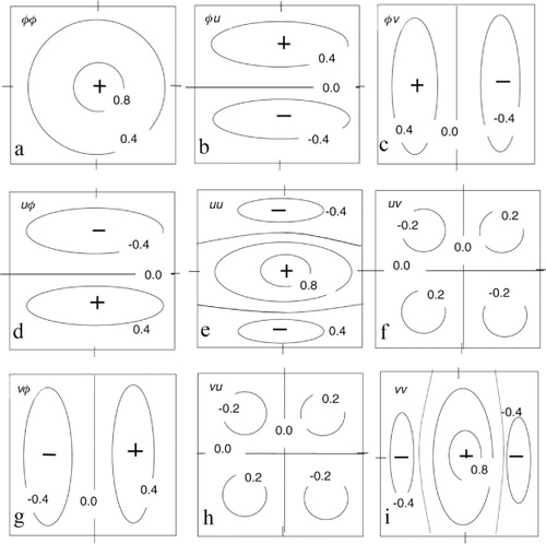
Figure 5 illustrates the correlation and cross-correlation functions for multivariate optimal interpolation analysis derived using the geostrophic increment assumption – after Gustafsson (1981) and Kalnay (2003). It demonstrates the response of the analysis increment from one variable (e.g. a geopotential or thermodynamic variable such as temperature) to another variable (e.g. u- and v- wind components), or vice versa. Comparing Figs. 3 and 4 with Fig. 5, it is apparent that the shapes of the analysis increments from 3DVAR over both mountainous and flat terrain follow classical correlation and cross-correlation functions of variables using the geostrophic increment assumption. If we count the changes of contour shapes due to the linear combination of the variables (i.e. Figs. 3e and 4e corresponding to the sum of Fig. 5e and 5f and so on), the shapes of the analysis increments revealed by Figs. 3 and 4 are equivalent to those structures in Fig. 5, showing the strong dependence of the 3DVAR analysis increments on the prescribed correlation functions in the background error covariance term.

Fig. 5.  Schematic illustration of the correlation and cross-correlation functions for multivariate OI analysis derived using the geostrophic increment assumption (courtesy Gustafsson 1981 and Kalnay 2003). ‘φ’ is thermodynamic variable related to the temperature. u and v denote the horizontal components of wind.

In addition, as shown in Fig. 3, the 3DVAR analysis increments from the observation station within the mountain valley area have been spread across the mountains. Since it is expected that the air temperature and wind conditions can be inhomogeneous over the mountain valley and cross-mountain areas, the cross-mountain analysis increments could be unrealistic. This feature of the cross-mountain analysis increment can be revealed even more clearly (although it is similar to Fig. 3) if we check the analysis increments at the 800 hPa pressure level (near the surface over the US Intermountain West; figure not shown).

In 3DVAR, the influence of a single observation on its surrounding area is determined by a horizontal correlation length-scale in the background error term [eq. (2)]. Fig. 6 shows the analysis increments of temperature at the model's lowest level from the assimilation of both 2-m temperature and 10-m wind with various background correlation length-scales. A simple sensitivity experiment indicates that a very small length-scale (25% of the default value that was specified in the NMC method when generating the B term for this study) is needed in order to avoid unrealistic cross-mountain analysis increments. However, with such a small length-scale, the analysis increment and the influence of the single observation could be minimised. Therefore, it is not realistic to use a very small length-scale. Meanwhile, since a relatively large length-scale has to be used, the 3DVAR method typically can have problems in assimilating data over complex terrain. Therefore, the length-scale is an influencing factor that could impose significant impact on the near-surface data assimilation with 3DVAR in the regions of complex terrain.

Fig. 6.  The 3DVAR analysis increments of temperature (K) with assimilation of both 2-m temperature and 10-m winds from a single observational station over complex terrain using different horizontal correlation length-scales: a default value (middle), 25% of the default value (left) and 150% of the default value (right). The shaded contour shows the terrain heights (m).

4.2. Ensemble Kalman filter

With the EnKF, the analysis increments resulted from observations at a single observational station over mountainous and flat terrain are shown in Figs. 7 and 8 (corresponding to Figs. 3 and 4 for 3DVAR), respectively. Compared with Figs. 3 and 4, the analysis increments from the EnKF are much more localised. They also have less correspondence with the correlation functions shown in Fig. 5. Since the EnKF defines the background error covariances using ensemble forecasts, Fig. 9 shows ensemble spreads of temperature, and u- and v- wind components over the area surrounding the observational station. The shapes and structures (in terms of magnitudes and gradients of the increment contour lines) of the analysis increments of temperature and u and v wind components from the EnKF correspond well to their ensemble spreads. Specifically, large analysis increments agree well with the large ensemble spread.

Fig. 7.  Same as Fig. 3, except for the EnKF analysis increments. The half radius of the horizontal localization used in the experiments is 320km. No vertical localization is applied.

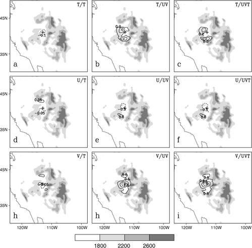
Fig. 8.  Same as Fig. 7, except over flat terrain.

Fig. 9.  Ensemble spread (shaded) and analysis increments (contour) for temperature (a; 0.1 K interval), u-component (b; 0.2 m s⁻¹ interval) and v-component (c; 0.2 m s⁻¹ interval) with assimilation of both 2-m temperature and 10-m wind using EnKF. The ‘+’ sign denotes the observational location.

More importantly, with the EnKF, over complex terrain the analysis increments resulting from the assimilation of observations in the valley remain inside the valley, unlike those with 3DVAR. No cross-mountain analysis increment is found (Fig. 7). In addition, similar to Fig. 3e and 3f (3h and 3i), Fig. 7e and 7f (7h and 7i) are very similar.

The spatial range of influence from an observation in the EnKF can be limited by the specification of the horizontal localisation scale. The sensitivity of analysis increments to the horizontal localisation radius has been tested. It is found that analysis results are sensitive to the horizontal localisation radius (Fig. 10). However, in the EnKF, even with a large localisation radius (Fig. 10c), the analysis increments from the valley station spread widely through the surrounding area but still remain mostly inside the valley.

Fig. 10.  Same as Fig. 6, except for EnKF with different radii of horizontal localization. The default value of half radius of the horizontal localization is 320 km (middle). The smaller (left) and larger (right) scales are 20% and 200% of the default value, respectively.

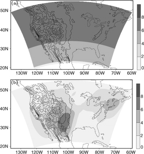
Overall, the major differences between the above experiments with 3DVAR and the EnKF can be attributed to differences in their background error terms. Since 3DVAR uses a fixed background term, analysis increments from a single observation tend to be similar in various cases, as they depend heavily on the prescribed correlation functions. The EnKF's flow-dependent background term enables the observations to have a greater influence on the areas where the ensemble spreads are larger. Figure 11a shows structures of the estimated background error standard deviation of the streamfunction in 3DVAR (static) and the EnKF averaged over the entire data assimilation period. In 3DVAR, the error variance is homogeneous in each statistical bin and has no correlation with terrain and the synoptic situation. In contrast, error variances in the EnKF reflect the structure of the synoptic system. As shown in Fig. 11b, large variances align well with the LLJ, indicating the flow-dependent nature of the EnKF background term.

Fig. 11.  Estimated background error standard deviation of the streamfunction (shaded contour; unit: 10⁵ m² s⁻¹) in 3DVAR (a, static in time) and EnKF [b, averaged over the data assimilation period (0000 UTC to 0600 UTC 5 June 2008)] near 800 m AGL. Contour lines denote the terrain heights (interval: 500m).

5. Experiments with multiple observations

The above results from assimilating observations from a single station show potential advantages of the EnKF over 3DVAR in assimilating near-surface observations. It is interesting to further explore whether the EnKF outperforms 3DVAR in short-range weather forecasting if only surface observations are assimilated. Surface observations have high spatial and temporal resolution and are among the most widespread observations of the lower atmosphere.

Therefore, we perform experiments, in which the observations from multiple stations (Fig. 2) are assimilated to examine and compare the ability of both 3DVAR and the EnKF to extend the information from single-level surface observations to the atmospheric boundary layer as well as to assess the impact on the short-range forecast. For experiments with both 3DVAR and EnKF, the data assimilation is performed for the period of 0000 UTC to 0600 UTC 5 June 2008, assimilating 2-m temperature and 10-m wind in a total of seven hourly data assimilation cycles. Then, 6-hour forecasts follow the data assimilation.

Sensitivity experiments are first conducted to determine the optimal length-scale for 3DVAR, and vertical and horizontal localisation scales for the EnKF. It is found that the default value of the length-scale, as defined by the NMC method, performs best for the 3DVAR method in terms of obtaining minimum root-mean-square errors for both analyses and forecasts. Three sets of experiments with various radii of maximum vertical localisation (i.e. 1000 m, 3000 m, 5000 m) for the EnKF are performed. Figure 12 shows the time-height root-mean-square errors of wind speed and temperature (against the nature run) over key LLJ and frontal regions. The 3000-m radius of maximum vertical localisation produces the best analysis/forecast. Similar sensitivity experiments are also conducted to determine the optimal horizontal localisation scale. Among several tested options (e.g. 120 km, 240 km, 360 km), a half-radius of the maximum horizontal localisation of 240 km is selected.

Fig. 12.  Time-height root-mean-square errors (against the nature run) of temperature (K; left column) averaged over a key front region and wind speed (m s⁻¹; right column) averaged over a key LLJ region, for EnKF experiments with various maximum radii of vertical localization scales: 1000m (a and b), 3000m (c and d), 5000m (e and f). The key frontal region and the key LLJ region are marked in Fig. 1b.

Based on the aforementioned sensitivity experiments, optimal results from 3DVAR and the EnKF are further discussed to compare their relative performance.

Figure 13 shows the wind direction and wind speed at 50 m AGL and temperature at 700 hPa at 0000 UTC 5 June 2008 after the first cycle of data assimilation with 3DVAR and EnKF. Compared with the corresponding fields in the nature run and control run (Fig. 1), the 3DVAR reproduced the LLJ system over the Great Plains but missed the cold frontal system over complex terrain. The EnKF, however, reproduced most parts of the cold front. The LLJ system is also well reproduced.

Fig. 13.  Same as Fig. 1, except for the 3DVAR (a) and EnKF (b) analysis after the first data assimilation cycle.

At the end of the data assimilation cycle, namely, at 0600 UTC 5 June 2008 (Fig. 14), 3DVAR results show only part of the frontal system, while sharing almost the full range of the LLJ but with weaker intensity in terms of wind speed. The EnKF captured the whole frontal system and more accurate intensity in terms of wind speed magnitude and the area of coverage of the LLJ. Overall, the EnKF performed better for both the LLJ and cold front cases. Further evaluations are conducted for the LLJ and cold front systems as follows.

Fig. 14.  Same as Fig. 1, except for 0600 UTC 05 June 2008 for nature run (a), control run (b), 3DVAR analysis (c), and EnKF analysis (d).

5.1. Low-level jet system over the Great Plains

We first evaluate the representation of the LLJ over the Great Plains during the data assimilation and forecast periods. Following Whiteman et al. (1997), the definition of the LLJ is when maximum wind speed reaches 12 ms⁻¹, with a fall-off value greater than 6 ms⁻¹ from the wind speed maximum upward to the next wind speed minimum at or below the 3000 m level. With the assimilation of surface observations, both 3DVAR and the EnKF are able to reproduce the LLJ system in the WRF model (e.g. Figs. 13 and 14).

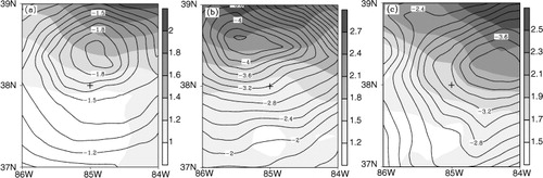
Figure 15 compares the wind profiles averaged over the key region of the LLJ from different experiments for 0000 UTC (beginning of the data assimilation cycle), 0600 UTC (end of the data assimilation cycle) and 1200 UTC (end of the forecast). It shows that both 3DVAR and EnKF resulted in an improved analysis and forecast of the LLJ, compared with the control run. Specifically, at the beginning of the data assimilation (0000 UTC), the EnKF results are clearly better than 3DVAR in terms of representing the magnitude of the mean wind speed, especially for the low level (up to a height of 1000 m). At the end of the data assimilation cycle (0600 UTC); both 3DVAR and the EnKF result in mean wind speeds that are close to the nature run at heights below 500 m. However, the maximum mean wind speed height is near 500 m in 3DVAR, while it is higher than 500m in both the EnKF and the nature run. After the 6-hour forecast (1200 UTC), results in 3DVAR and the EnKF are still closer to the nature run than those in the control run. Compared with 3DVAR, the EnKF analysis leads to a better forecast in terms of the vertical structure of the mean wind speed and the height of the maximum wind speed over the LLJ area.

Fig. 15.  Vertical profiles of mean wind speed (m s⁻¹) over the key regions of LLJ. Over a box of (32°N–38°N; 103°W–97°W) after the first data assimilation cycle at 0000 UTC 5 June 2008 (a), (28°N–38°N; 103°W–95°W) at the end of data assimilation cycle at 0600 UTC 5 June 2008 (b), and (32°N–40°N; 105°W–95°W) after 6 h forecast at 1200 UTC 5 June 2008 (c).

5.2. A cold front over complex terrain

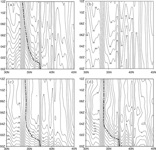
A cold front is passing over the Intermountain West (complex terrain) during the study period. Figure 16 shows the time-latitude cross-section of temperature averaged over the main frontal area (6° longitude ranging from 114°W to 108°W) at 500 m AGL. In contrast to the nature run, the control run missed the major cold front. With both 3DVAR and EnKF, the frontal system is reproduced although the temperature over the frontal region in both the 3DVAR and EnKF experiments is higher than that in the nature run. However, compared with 3DVAR, the temperature in the EnKF experiment is closer to that in the nature run over the frontal area.

Fig. 16.  Time-latitude cross-section of temperature averaged over the main front zone in 6° longitude ranging from 114°W to 108°W at 500 m AGL for nature run (a), control run (b), 3DVAR analysis (c), and EnKF analysis (d). The dashed bold lines denote the cold front.

To further compare the 3DVAR and EnKF experiments during the analysis and forecast period, Fig. 17 illustrates the differences in the root-mean-square errors (data assimilation experiments against the nature run) between the EnKF and 3DVAR for both the temperature and wind fields (the negative numbers indicate that the analysis or forecast errors in the EnKF are less than those in 3DVAR). Here, the root-mean-square errors are calculated over all observation stations in the key frontal region over a box of [20°N–45°N; 120°W–100°W]. The figure clearly reveals that the EnKF performs better than 3DVAR at all height levels in both the analysis and forecast periods.

Fig. 17.  The time-height differences of the root-mean-square (RMS) errors (against the nature run) between EnKF and 3DVAR for (a) temperature (K) and (b) wind speed (m s⁻¹), calculated over all stations in the key front region as marked in Fig. 1b. The negative numbers imply EnKF has smaller RMS errors, relative to 3DVAR.

6. The impact of terrain representation on surface data assimilation

Terrain mismatch – namely, the discrepancy between model and realistic terrain heights – is common in numerical models over complex terrain due to the limitation of model resolution in resolving detailed terrain features. In order to test the impact of this type of terrain mismatch on surface data assimilation, we perform an additional set of experiments, in which terrain heights are perturbed by using coarser resolution terrain (2-degree vs. 10-minute resolution) in the control and data assimilation experiments. In addition, a common way to deal with the terrain misrepresentation is to reject the data over the area where discrepancies between the model and realistic terrain are large. Therefore, another set of experiments is conducted, in which we reject the data when terrain differences between the experiments and nature run are greater than 25 m. Figure 18 shows the stations where the surface data are rejected in data assimilation. Since observations at many stations are rejected in mountainous region as seen in Fig. 18, the length scale in 3DVAR and the horizontal localisation scale in EnKF need to be adjusted to adapt to changes of the density of observations being assimilated. Sensitivity experiments are conducted with increased length scales in 3DVAR and localisation scales in EnKF to determine the new optimal scales. By comparing the RMS errors from these sensitivity experiments, the length (localisation) scale that produced the smallest RMS errors in 3DVAR (EnKF) is chosen as a new optimal scale to produce data assimilation results for further comparison.

Fig. 18.  Same as Fig. 2, except triangle signs denote rejected stations.

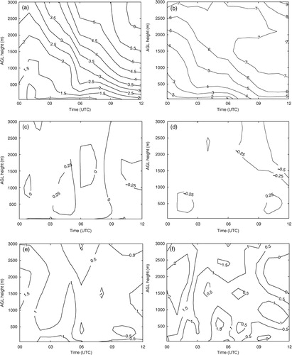
Figure 19 illustrates results from the EnKF. Compared with the RMS errors of temperature and wind in the boundary layer over the key frontal region (complex terrain) in the original (default) experiment (as mentioned in Section 5, without perturbing the terrain heights and data rejection; Fig. 19a and b), the EnKF analysis and subsequent forecasts with perturbed terrain heights achieve very similar accuracy, as the discrepancies in RMS errors between two experiments (Fig. 19c and d) are almost negligible. This result indicates that the EnKF has a good ability to handle the terrain mismatch. However, when the data are rejected over the areas of terrain mismatch, the data assimilation and forecast results are degraded (Fig. 19e and f). Since there are fewer observation stations over complex terrain in the western US than in the eastern US, the degraded analysis and forecast here can be attributed to the lack of data over complex terrain.

Fig. 19.  Time-height root-mean-square (RMS) errors (against the nature run) of temperature (K; left column) and wind speed (m s⁻¹; right column) for EnKF analysis and subsequent forecast in the key front region as marked in Fig. 1b. For the default experiment without terrain perturbation and data rejection (a and b); RMS error differences between the experiment with terrain perturbation and default experiment (c and d; positive numbers denote the degraded analysis and forecast from the experiment with terrain perturbation); and the RMS error differences between the experiment with data rejection and the default experiment (positive numbers mean the degraded analysis and forecast from the data rejection experiment).

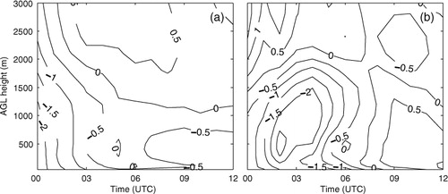
Outcomes from the 3DVAR experiments show that the data assimilation results were degraded under mismatched terrain, compared with the results before perturbing the terrain (figure not shown), indicating that 3DVAR has less ability to handle the mismatched terrain than the EnKF does. In addition, under the data rejection case, 3DVAR results are even worse than those from the EnKF (Fig. 20).

Fig. 20.  Same as Fig. 17, except for the data rejection experiment.

7. Concluding remarks

Although surface observations are the main source of conventional observations and have been very important for weather forecasting, their use in modern NWP, especially over complex terrain, remains a unique challenge. In this study, a series of OSSEs is performed with two popular data assimilation methods, a 3DVAR and an EnKF. The problems and advantages of both methods in assimilating near-surface observations are examined.

Even with a single case study, results from this study reproduce many details that explain the differences between the 3DVAR and the EnKF in the context of surface data assimilation. Results from the assimilation of surface 2-m temperature and 10-m wind from a single observation station demonstrate that there are fundamental problems in assimilating surface observations over complex terrain using 3DVAR. Specifically, the analysis increments from a valley station can unrealistically spread over the mountain areas even with a reasonable specification of the horizontal background length-scale. The EnKF can overcome some of these limitations through its flow-dependent background error term. Overall, major discrepancies between 3DVAR and the EnKF in the single observation influence can be attributed to their different ways of defining the background error term. Since 3DVAR uses a fixed background term, analysis increments from a single observation tend to be similar in various cases as they depend heavily on the prescribed correlation functions. Owing to its flow-dependent background error covariance term, the EnKF enables observations to have more influence on areas where the ensemble spreads are larger. In addition, due to sampling errors with limited ensemble size, data assimilation results from the EnKF are sensitive to the choice of the horizontal and vertical localisation scales.

More comprehensive comparisons are conducted using a synoptic case with two severe weather systems: a front over complex terrain in the western US and a low-level jet over the Great Plains. It is found that both 3DVAR and the EnKF are capable of extending information from surface observations to the atmospheric boundary layer. Over flat terrain, the EnKF does better in terms of the analysis and forecast of the low-level jet system while the 3DVAR also simulates the low-level jet system generally well. Over complex terrain, the EnKF performs much better than 3DVAR in general. Specifically, the EnKF has a better ability to handle surface data under terrain misrepresentation. Since a common way to deal with terrain misrepresentation is to reject data over the area where discrepancies between the model and the actual terrain are large, a data-rejection experiment is performed. However, since data are sparse over complex terrain, data rejection results in degraded analyses and forecasts, suggesting that this may not be the best solution for dealing with errors due to model terrain representation.

It should be noted that the OSSEs performed in this paper are in idealised settings in order to isolate various factors that affect the assimilation of near-surface observations. In addition, the terrain data used in OSSEs are all from model terrain, which is much smoother than the actual terrain. Therefore, while the results in this study can help us understand what factors limit our ability to assimilate surface data, the real data assimilation and prediction problems are expected to be more complicated. Future work will further investigate the problems and challenges in assimilating surface observations over complex terrain with real observations and realistic terrain with many cases. Additional experiments will also be performed at high-resolution in nested domains, as significant surface analysis and forecast improvements are found when the EnKF grid spacing is reduced (e.g. Ancell et al., 2011).

In addition, hybrid 3DVAR and EnKF data assimilation schemes (e.g. Hamill and Snyder, 2000; Wang et al., 2008) have been developed in both research and operational communities. There are hopes that these hybrid data assimilation systems could overcome some deficiencies of the 3DVAR method. Meanwhile, a four-dimensional variational data assimilation (4DVAR) method is also widely used for operational prediction. Future work will evaluate the ability of the hybrid data assimilation systems and 4DVAR in assimilating near-surface observations.

Furthermore, model errors from land-atmosphere thermal coupling could be another issue in near-surface data assimilation. In a recent study with a single column model, Hacker and Angevine (2012) suggest that the parameterisation error that accounts for the inaccurate representation of thermal coupling between land and atmosphere is difficult to estimate. They also pointed out that soil and flux measurements have large impacts on near surface variables. Therefore, future studies should also pay attention to the role of model errors in near-surface data assimilation.

8. Acknowledgments

The authors are grateful to the NCAR WRF model development group and Data Assimilation Research Testbed (DART) team. Specifically, they would like to thank Glen Romine, Nancy Collins and Hui Liu for their help in the use of the DART/WRF. The first author (ZP) would also like to express thanks to Prof Eugenia Kalnay at the University of Maryland and Dr Geoff DiMego at NCEP for their early encouragement in working on the surface data assimilation. Review comments from Dr Joshua Hacker and two anonymous reviewers are highly appreciated, as they are helpful for improving the manuscript. This study is supported by Office of Science (BER), U.S Department of Energy Grant No. DE-SC0007060, National Science Foundation Grant AGS-08339856 and AGS-1243027, and the Office of Naval Research Award No. N00014-11-1-0709. The computer support from the Centre for High Performance Computing (CHPC) at the University of Utah is also gratefully acknowledged.

References

- Ancell B. C. Mass C. F. Hakim G. J. Evaluation of surface analyses and forecasts with a multiscale ensemble Kalman filter in regions of complex terrain. Mon. Wea. Rev. 2011; 139: 2008–2024. 10.3402/tellusa.v65i0.19620.
- Anderson J. L. An ensemble adjustment Kalman filter for data assimilation. Mon. Wea. Rev. 2001; 129: 2884–2903.
- Anderson J. L. A local least squares framework for ensemble filtering. Mon. Wea. Rev. 2003; 131: 634–642.
- Anderson J. L. An adaptive covariance inflation error correction algorithm for ensemble filters. Tellus A. 2007; 59: 210–224. 10.3402/tellusa.v65i0.19620.
- Anderson J. L. Localization and sampling error correction in ensemble Kalman filter data assimilation. Mon. Wea. Rev. 2012; 140: 2359–2371. 10.3402/tellusa.v65i0.19620.
- Anderson J. L. Hoar T. Raeder K. Liu H. Collins N. co-authors. The data assimilation research testbed: A community facility. Bull. Amer. Meteor. Soc. 2009; 90: 1283–1296. 10.3402/tellusa.v65i0.19620.
- Barker D. M. Huang W. Guo Y. R. Bourgeois A. J. Xiao Q. N. A three dimensional data assimilation system for use with MM5: Implementation and initial results. Mon. Wea. Rev. 2004b; 132: 897–914.
- Barker, D. M, Lee, M.-S, Guo, Y.-R, Huang, W, Xiao, Q.-N and Rizvi, R. 2004a. WRF variational data assimilation development at NCAR. In: WRF/MM5 Users’ Workshop. June 22–25, 2004. Boulder: CO. Online at: http://www.mmm.ucar.edu/mm5/workshop/workshop-papers_ws04.html.
- Benjamin S. G. Devenyi D. Weygandt S. Brundage K. J. Brown J. co-authors. An hourly assimilation-forecast cycle: the RUC. Mon. Wea. Rev. 2004; 132: 495–518.
- Benjamin, S. G, Weygandt, S, Smirnova, T, Alexander, C, Hu, M. and co-authors. 2011. Progress in NOAA hourly-updated models – Rapid Refresh, HRRR. A presentation to Alaska Weather Symposium, March 15, 2011, Fairbanks: AK.
- Bishop C. H. Etherton B. J. Majumdar S. J. Adaptive sampling with the ensemble transform Kalman filter. Part I: theoretical aspects. Mon. Wea. Rev. 2001; 129: 420–436.
- Buehner M. Evaluation of a spatial/spectral covariance localization approach for atmospheric data assimilation. Mon. Wea. Rev. 2012; 140: 617–636. 10.3402/tellusa.v65i0.19620.
- Chen Y. Snyder C. Assimilating vortex position with an ensemble Kalman filter. Mon. Wea. Rev. 2007; 135: 1828–1845. 10.3402/tellusa.v65i0.19620.
- Courtier P. Thépaut J.-N. Hollingsworth A. A strategy for operational Implementation of 4D-Var, using an incremental approach. Q. J. Roy. Meteor. Soc. 1994; 120: 1367–1387. 10.3402/tellusa.v65i0.19620.
- Daley R. Atmospheric Data Analysis. Cambridge University Press, Cambridge, UK, 457.1991
- De Pondeca M. S. F. V. Manikin G. S. DiMego G. Benjamin S. G. Parrish D. F. co-authors. The real-time mesoscale analysis at NOAA's National Centers for Environmental Prediction: current status and development. Wea. Forecasting. 2011; 26: 593–612. 10.3402/tellusa.v65i0.19620.
- DiMego, G. 2006. Implementation brief: real-time mesoscale analysis (RTMA), Presentation on 9 August 2006, NOAA/NWS [Powerpoint file available upon request].
- Dong, J, Xue, M and Droegemeier, K. 2007. The impact of high-resolution surface observation on convective storm analysis with ensemble Kalman filter. In: 22nd Conference on Weather Analysis and Forecasting/18th Conference on Numerical Weather Prediction. Park City: UtahAMS, CDROM P1.42.
- Evensen G. Sequential data assimilation with a nonlinear quasi-geostrophic model using Monte Carlo methods to forecast error statistics. J. Geophys. Res. 1994; 99: 10143–10162. 10.3402/tellusa.v65i0.19620.
- Evensen G. Data Assimilation – The Ensemble Kalman Filter. Springer-Verlag, Berlin, Heidelberg, 279.2007
- Fujita T. Stensrud D. J. Dowell D. C. Surface data assimilation using an ensemble Kalman filter approach with initial condition and model physical uncertainties. Mon. Wea. Rev. 2007; 135: 1846–1868. 10.3402/tellusa.v65i0.19620.
- Gandin, L. S. 1963. Objective analysis of meterological fields, Gidrometerologicheskoe Izdatelstvo, Leningrad. English translation by Israeli program for scientific translation, Jerusalem, 1965.
- Gustafsson, N. 1981. A review of methods for objective analysis. In: Dynamic Medeorology: Data Assimilation Methods. L.Bengtsson, M.Ghil and E.Källen, Springer-Verlag: New York, pp. 17–76.
- Hacker J. P. Anderson J. L. Pagowski M. Improved vertical covariance estimates for ensemble-Filter assimilation of near-surface observations. Mon. Wea. Rev. 2007; 135: 1021–1036. 10.3402/tellusa.v65i0.19620.
- Hacker, J. P and Angevine, W. M. 2012. Ensemble data assimilation to characterize land-atmosphere coupling errors in numerical weather prediction models. Mon. Wea. Rev. (in press).
- Hacker J. P. Snyder C. Ensemble Kalman filter assimilation of fixed screen-height observations in a parameterized PBL. Mon. Wea. Rev. 2005; 133: 3260–3275. 10.3402/tellusa.v65i0.19620.
- Hamill T. M. Snyder C. A hybrid ensemble Kalman filter–3D variational analysis scheme. Mon. Wea. Rev. 2000; 128: 2905–2919.
- Hamill T. M. Whitaker J. Snyder C. Distance-dependent filtering of background error covariance estimates in an ensemble Kalman filter. Mon. Wea. Rev. 2001; 129: 2776–2790.
- Houtekamer P. L. Mitchell H. L. Data assimilation using an ensemble Kalman filter technique. Mon. Wea. Rev. 1998; 126: 796–811.
- Houtekamer P. L. Mitchell H. L. A sequential ensemble Kalman filter for atmospheric data assimilation. Mon. Wea. Rev. 2001; 129: 123–137.
- Kalnay E. Atmospheric Modeling, Data Assimilation and Predictability. Cambridge University Press, Cambridge, UK, 341.2003
- Kalnay E. Kanamitsu M. Kistler R. Collins W. Deaven D. co-authors. The NCEP/NCAR 40-year reanalysis project. Bull. Amer. Meteor. Soc. 1996; 77: 437–471.
- Lee, S.-J, Parrish, D. F, Wu, W.-S, De Pondeca, M, Keyser, D. and co-authors. 2005. Use of surface mesonet data in NCEP regional grid statistical-interpolation system. Preprints. In: AMS 17th Conference on Numerical Weather Prediction. American Meteorological Society: Washington, DC, 1–5 August, 2005.
- Lewis J. M. Lakshmivarhan S. Dhall S. K. Dynamic Data Assimilation: A Least Squares Approach. Cambridge University Press, Cambridge, UK, 654.2006
- Lorenc A. Analysis methods for numerical weather prediction. Q. J. R. Meteorol. Soc. 1986; 112: 1177–1194. 10.3402/tellusa.v65i0.19620.
- Meng Z. Zhang F. Tests of an ensemble Kalman filter for mesoscale and regional-scale data assimilation. Part IV: comparison with 3DVAR in a month-long experiment. Mon. Wea. Rev. 2008a; 136: 3671–3682. 10.3402/tellusa.v65i0.19620.
- Meng Z. Zhang F. Tests of an ensemble Kalman filter for mesoscale and regional-scale data assimilation. Part III: comparison with 3DVAR in a real-data case study. Mon. Wea. Rev. 2008b; 136: 522–540. 10.3402/tellusa.v65i0.19620.
- Mesinger F. DiMego G. Kalnay E. Mitchell K. Shafran P. C. co-authors . North American regional reanalysis. Bull. Amer. Meteor. Soc. 2006; 87: 343–360. 10.3402/tellusa.v65i0.19620.
- Miyoshi T. The Gaussian approach to adaptive covariance inflation and its implementation with the local ensemble transform Kalman filter. Mon. Wea. Rev. 2011; 139: 1519–1535. 10.3402/tellusa.v65i0.19620.
- Parrish D. F. Derber J. C. The National Meteorological Center's spectral statistical interpolation analysis system. Mon. Wea. Rev. 1992; 120: 1747–1763.
- Rogers, E, Ek, M, Ferrier, B. S, Gayno, G, Lin, Y. and co-authors. 2005. The NCEP North American Mesoscale Modeling System: Final Eta model/analysis changes and preliminary experiments using the WRF-NMM. In: 17th Conference on Numerical Weather Prediction. Washington: DCAMS, August 1–5, 2005.
- Simmons, A. J, Jones, P. D, Bechtold, V. D, Beljaars, A. C. M, Kallberg, P. W. and co-authors. 2004. Comparison of trends and low-frequency variability in CRU, ERA-40, and NCEP/NCAR analyses of surface air temperature. J. Geophys, Res. 109, D24115., 10.3402/tellusa.v65i0.19620.
- Skamarock, W. C, Klemp, J. B, Dudhia, J, Gill, D. O, Barker, D. M. and co-authors. 2008. A Description of the Advanced Research WRF Version 3. NCAR Tech. Note NCAR/TN-475+STR, 113. pp.
- Stensrud D. Yussouf N. Dowell D. Coniglio M. Assimilating surface data into a mesoscale model ensemble: Cold pool analyses from spring 2007. Atmos. Res. 2009; 93: 207–220. 10.3402/tellusa.v65i0.19620.
- Tippett M. K. Anderson J. L. Bishop C. H. Hamill T. M. Whitaker J. S. Ensemble square root filters. Mon. Wea. Rev. 2003; 131: 1485–1490.
- Torn R. D. Performance of a mesoscale ensemble Kalman filter (EnKF) during the NOAA high-resolution hurricane test. Mon. Wea. Rev. 2010; 138: 4375–4392. 10.3402/tellusa.v65i0.19620.
- Torn R. D. Hakim G. J. Snyder C. Boundary conditions for limited-area ensemble Kalman filters. Mon. Wea. Rev. 2006; 134: 2490–2502. 10.3402/tellusa.v65i0.19620.
- Wang X. Barker D. M. Snyder C. Hamill T. M. A Hybrid ETKF–3DVAR Data Assimilation Scheme for the WRF Model. Part II: Real Observation Experiments. Mon. Wea. Rev. 2008; 136: 5132–5147. 10.3402/tellusa.v65i0.19620.
- Whitaker J. S. Hamill T. M. Ensemble data assimilation without perturbed observations. Mon. Wea. Rev. 2002; 130: 1913–1924.
- Whiteman C. D. Bian X. Zhong S. Low-level jet climatology from enhanced rawinsonde observations at a site in the southern Great Plains. J. Appl. Meteor. 1997; 36: 1363–1376.
- Wu W.-S. Purser R. J. Parrish D. F. Three-dimensional variational analysis with spatially inhomogeneous covariances. Mon. Wea. Rev. 2002; 130: 2905–2916.
- Xie, Y, Koch, S. E, McGinley, J. A, Albers, S and Wang, N. 2005. A sequential variational analysis approach for mesoscale data assimilation. In: AMS 21st Conference on Weather Analysis and Forecasting/17th Conference on numerical weather prediction. Paper 15B.7. Online at: https://ams.confex.com/ams/WAFNWP34BC/techprogram/programexpanded_299.htm.