Effective assimilation of global precipitation: simulation experiments

Abstract

Past attempts to assimilate precipitation by nudging or variational methods have succeeded in forcing the model precipitation to be close to the observed values. However, the model forecasts tend to lose their additional skill after a few forecast hours. In this study, a local ensemble transform Kalman filter (LETKF) is used to effectively assimilate precipitation by allowing ensemble members with better precipitation to receive higher weights in the analysis. In addition, two other changes in the precipitation assimilation process are found to alleviate the problems related to the non-Gaussianity of the precipitation variable: (a) transform the precipitation variable into a Gaussian distribution based on its climatological distribution (an approach that could also be used in the assimilation of other non-Gaussian observations) and (b) only assimilate precipitation at the location where at least some ensemble members have precipitation. Unlike many current approaches, both positive and zero rain observations are assimilated effectively.

Observing system simulation experiments (OSSEs) are conducted using the Simplified Parametrisations, primitivE-Equation DYnamics (SPEEDY) model, a simplified but realistic general circulation model. When uniformly and globally distributed observations of precipitation are assimilated in addition to rawinsonde observations, both the analyses and the medium-range forecasts of all model variables, including precipitation, are significantly improved as compared to only assimilating rawinsonde observations. The effect of precipitation assimilation on the analyses is retained on the medium-range forecasts and is larger in the Southern Hemisphere (SH) than that in the Northern Hemisphere (NH) because the NH analyses are already made more accurate by the denser rawinsonde stations. These improvements are much reduced when only the moisture field is modified by the precipitation observations. Both the Gaussian transformation and the new observation selection criterion are shown to be beneficial to the precipitation assimilation especially in the case of larger observation errors. Assigning smaller horizontal localisation length scales for precipitation observations further improves the LETKF analysis.

• ensemble Kalman filter
• data assimilation
• precipitation
• non-Gaussianity
• anamorphosis

1. Introduction

Precipitation has long been one of the most important and useful meteorological quantities to observe. The traditional rain gauge measurement of precipitation can be traced back to the 19th century before the rawinsonde network was established (e.g. Jones and Bradley, 1992). In recent years, more advanced precipitation estimations from a variety of remote-sensing platforms, such as satellite and ground-based precipitation radar, have also become available. For example, the Tropical Rainfall Measuring Mission (TRMM) has been used to produce a set of high-quality, high-resolution global (50S–50N) precipitation estimates (Huffman et al., 2007) that have been widely used in many research areas. The Global Precipitation Measurement (GPM; Hou et al., 2008) mission is scheduled for launch in 2014 as the successor to TRMM. Because of the large impact that effective assimilation of precipitation could have in forecasting severe weather (Bauer et al., 2011), many efforts to assimilate precipitation observations have been made.

Both nudging and variational methods have been used previously to assimilate precipitation by modifying the model's moisture and sometimes temperature profiles as well, in order to either enhance or reduce short-term precipitation according to the model parameterisation of rain (e.g. Tsuyuki, 1996, 1997; Falkovich et al., 2000; Davolio and Buzzi, 2004; Koizumi et al., 2005; Mesinger et al., 2006). They are generally successful in forcing the forecasts of precipitation to be close to the observed precipitation during the assimilation, but the resulting forecast perturbations quickly decay. For example, a nudging method was applied to the North American Regional Reanalysis (NARR), and achieved the objective of making the Eta NARR 3-h forecasts essentially identical to the observed precipitation used to nudge the model (Mesinger et al., 2006). However, the Eta forecasts from the NARR were not superior to the operational forecasts beyond a few hours. Nudging the moisture was not effective presumably because it is not an efficient way to update the potential vorticity field, which is the ‘master’ dynamical variable that primarily determines the evolution of the forecast in NWP models.

There are other important issues for precipitation assimilation in the variational framework. Precipitation processes parameterised by the model physics are usually very non-linear and even discontinuous at some ‘thresholds’ (Zupanski and Mesinger, 1995). Therefore, it is problematic to create and use the linearised version of the forward model as required in the 4D-Var assimilation of precipitation variables (Errico et al., 2007). An inaccurate tangent linear model and adjoint model would yield a poor estimate of the evolution of finite perturbations and degrade the 4D-Var analyses. Considerable efforts have been made on improving the model's moist physics in order to improve the assimilation of precipitation remotely sensed by satellite or radar (e.g. Treadon et al., 2003; Li and Mecikalski, 2010, 2012). Alternative moist physical parameterisation schemes that are more linear and continuous have been used to reduce the non-linearity problem (e.g. Zupanski and Mesinger, 1995; Lopez and Moreau, 2005). In addition, the highly non-Gaussian distribution of the precipitation observations seriously violates the basic assumption of normal error statistics made in most data assimilation schemes. The flow-independent background error covariance that is usually used in variational methods cannot describe the relationship between precipitation and other state variables. All of these problems have contributed to the difficulties of the precipitation assimilation, leading to a widely shared experience that forecasts starting from analyses with precipitation assimilation lose their extra skill in forecasts of precipitation or other dynamical variables after just a few forecast hours (e.g. Davolio and Buzzi, 2004; Errico et al., 2007; Tsuyuki and Miyoshi, 2007). One notable exception is Hou et al. (2004) who used forecast tendency corrections of temperature and moisture as control variables in variational data assimilation in the assimilation of hurricane observed precipitation. They were able to show that large changes in precipitation had long-lasting positive impacts on a hurricane forecast, presumably because the release of latent heat corrected the potential vorticity.

Bauer et al. (2011) recently reviewed the current status of precipitation assimilation and concluded that there are still major difficulties related to (1) the moist physical processes in NWP models and their linear representation and (2) the non-Gaussianity of both precipitation observations and model perturbations. Here, we propose to use the ensemble Kalman filter (EnKF) method to address these critical issues. It is noted that an accurate moist physical parameterisation scheme is essential for effective precipitation assimilation. The EnKF method does not require linearisation of the model or any other modification of the model physics as required in variational methods. Instead, we use the original model parameterisation scheme in the ensemble forecast step. Furthermore, an accurate precipitation parameterisation should result in useful error covariances between the diagnostic precipitation and the state variables in the background forecast ensemble, and a useful assimilation of precipitation. The ensemble approach should be able to more efficiently change the potential vorticity field by allowing ensemble members with better precipitation (due to presumably better dynamics) to locally have greater influence (i.e. receive higher weights) in the analysis step. Several pioneering experiments of precipitation assimilation using EnKF methods have already been conducted (Miyoshi and Aranami, 2006; Zupanski et al., 2011; Zhang et al., 2013) with encouraging results.

The non-Gaussianity issue has also been a critical problem. Bocquet et al. (2010) provided a comprehensive review of the methods to deal with the non-Gaussianity in various data assimilation schemes. Previously, transformations such as a logarithmic transformation have been applied to the precipitation assimilation (e.g. Hou et al., 2004; Lopez, 2011). Although the logarithmic transformation is expected to alleviate the non-Gaussianity of positive precipitation, it is not necessarily optimal. In this study, we propose to use a general variable transformation algorithm (i.e. Gaussian anamorphosis; Wackernagel, 2003), which can transform any continuously distributed variable into a Gaussian distribution based on its empirical (climatological) distribution. In addition, we also address the use of observations of zero precipitation. Past studies have shown that it is very difficult to achieve improvement by assimilation of zero-precipitation observations in the usually used methods (e.g. Tsuyuki and Miyoshi, 2007). However, as shown in Weygandt et al. (2008), the forced suppression of convection in areas with no radar echoes did show the importance of zero-precipitation observations in correctly analysing a convection system. We propose here a new criterion based on the model background that allows some zero-precipitation observations to be assimilated. The only condition required in order to assimilate precipitation observations is that at least several background ensemble members have positive precipitation, regardless of the observed values. Our results suggest this criterion is useful in order to exploit the value of zero-precipitation observations, probably in areas of scattered precipitation or at the edge of large-scale areas of precipitation.

In this article, we use a relatively simple but realistic system to test the above ideas. Identical-twin observing system simulation experiments (OSSEs) with a simplified global circulation model (GCM) are the framework of this study. Previously, using the same OSSE framework, but without introducing the Gaussian transformation (GT) of precipitation and the new criterion for precipitation assimilation, analysis and forecast errors became significantly larger when precipitation was assimilated. Therefore, success demonstrated here using a simple forecast model provides motivation to apply our approach in more complicated systems.

This article is organised as follows. The methodology including the GT and special treatment of zero-precipitation observations are introduced in Section 2. Section 3 describes the model, the local ensemble transform Kalman filter (LETKF) used in this study, and the detailed settings of the OSSEs. Section 4 presents the results of the precipitation assimilation. Section 5 contains concluding remarks and further discussions.

2. Methodology for an effective assimilation of precipitation with an EnKF

2.1. Gaussian transformation

In order to satisfy the basic assumption of Gaussian distribution and error statistics in data assimilation, we seek a general transformation algorithm to transform any variable y with a known arbitrary distribution into a standard Gaussian variable y _trans. This can be achieved through the connection between the two cumulative distribution functions (CDFs) of y and y _trans:1 where F(y) represents the CDF of y (by definition having values from 0 to 1), and G ⁻¹ is the inverse CDF of a normal distribution with zero mean and unit standard deviation such as y _trans is designed to be. Here,2

where erf⁻¹ is the inverse error function. The CDF of y can be determined empirically. In this study, we first run the Simplified Parametrisations, primitivE-Equation DYnamics (SPEEDY) model for 10 yr and in order to compute the CDF of precipitation variables (6-h accumulated precipitation) at each grid point and at each season based on this 10-yr model climatology. Transformations of both observation and model precipitation variables are thus made in terms of their spatial location and season during the assimilation process. This technique is called ‘Gaussian anamorphosis’ (e.g. Wackernagel, 2003) and has been also used in some geophysical data assimilation studies (e.g. Simon and Bertino, 2009; Schöniger et al., 2012). Note that this method transforms the climatological distribution of the original variable into a Gaussian distribution as a whole, but not its error distribution at every measurement and model background. Nevertheless, we assume that the error distribution in a more Gaussian variable would also have more Gaussian error statistics, and test whether this method is actually beneficial in the experimental results.

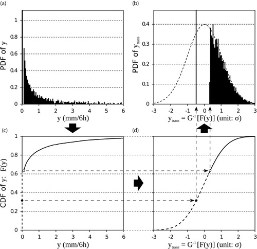
The transformation ensures a simple one-to-one relationship between the original variable and the transformed variable if their CDFs are continuous. Figure 1 illustrates how the transformation works for the precipitation distribution at a grid point near Maryland in the winter season. The probability density function (PDF) and CDF [i.e. F(y)] of the original precipitation variable are shown in Fig. 1a and c, respectively. Using the inverse CDF of normal distribution G ⁻¹, the F(y) is converted back to the transformed variable y _trans, with the CDF shown in Fig. 1d and the PDF in Fig. 1b. It is apparent that the precipitation is not a continuous variable since it contains a large portion of zero values so that the CDF is discontinuous at zero. The dashed parts of lines in Fig. 1b–d are associated with those zero-precipitation values. This issue will be addressed and the figure will be further discussed in the next section. Note that multimodal distributions would not pose any difficulty in defining the transformation.

Fig. 1 The PDF and CDF of (a, c) the original precipitation and (b, d) the transformed precipitation at a grid point near Maryland (38.967°N, 78.75°W) in winter season (December–February) based on the 10-yr nature run. The procedure of the GT is from (a) to (c), to (d), and to (b) as indicated by the arrows.

PDF = probability density function; CDF = cumulative distribution function; GT = Gaussian transformation.

In addition, G ⁻¹ will transform zero and one to −∞ and +∞ respectively, suggesting that the outliers of precipitation values will cause problems. In order to avoid problems transforming those outliers, we set all precipitation values with cumulative distribution less than 0.001 and greater than 0.999 to the values 0.001 and 0.999, respectively. This only affects very few values that are close to the tails of the model climatological distribution or that may even fall outside the distribution. Consequently, they will be transformed into −3.09 and 3.09.

2.2. Treatment of zero precipitation

As mentioned in the previous section, precipitation variables contain a large portion of zero values, which is manifested as a delta function in the PDF (Fig. 1a). As any deterministic transformation of a delta function will still result in a delta function, it would be impossible to obtain a transformed precipitation variable with perfect normal distribution if all precipitation values are considered. A naïve approach would be to only transform the non-zero part of precipitation data. However, this is not practical in data assimilation because even if all zero-precipitation observations are discarded, in the background forecast there may be zero values at the corresponding observation location which still need to be transformed (via the observation operator) before they are passed into the assimilation calculation. In ensemble data assimilation framework, this problem is even more apparent than in variational data assimilation since it is very likely that a random ensemble member would have zero precipitation at an observation location. Therefore, a heuristic solution to the transform of zero-precipitation values is necessary.

In our proposed algorithm, the CDF F(y) is discontinuous at y=0, thus the problem with zero precipitation in this algorithm is equivalent to assigning a value of cumulative probability F for zero precipitation (y=0). In the absence of an ideal solution, a reasonable choice is to assign the middle value of zero-precipitation cumulative probability to F(0). In the example shown in Fig. 1c and d, the probability of zero precipitation is about 63.4% (CDF=0.634 for minimum positive precipitation; open circles), thus F(0) = 0.317 is assigned for all zero precipitation (solid circles) at that grid point. In this way, the zero precipitation in the transformed variable is still a delta function in its PDF (Fig. 1b), but it is located at the median of the zero-precipitation part of the normal distribution. Therefore, though not perfectly Gaussian, it is more reasonable than the original skewed distribution. We tested other more sophisticated approaches, including one that assigned uniformly distributed random values to fill up the zero-precipitation cumulative probability so that a perfect Gaussian variable could be generated, but their experimental impacts in the assimilation experiments were no better than that of the simple median approach.

We note that traditional precipitation assimilation systems in the variational framework usually discard the zero-precipitation observations (e.g. Koizumi et al., 2005) because those observations are difficult to use. Nevertheless, zero-precipitation observations should contain valuable (and accurate) information about the atmospheric state. With our current transformation algorithm handling the zero precipitation and an ensemble data assimilation system, zero-precipitation observations are, indeed, assimilated. Instead of discarding zero observations, a different criterion is used in this study: assimilation is conducted at all grid points where at least some members of prior ensemble are precipitating (regardless of the observed values). This is because if the ensemble spread is zero (i.e. all forecasts have zero precipitation), it is not possible to assimilate precipitation using an EnKF. In Section 4.1, we will show that assimilating precipitation observations at locations with only a few precipitating members does not show improvements so that the criterion we have chosen is to require that at least half of the forecasts have positive precipitation, which controls the assimilation quality and saves computational time. We will also show that while this model background-based criterion only allows us to assimilate a small portion of the zero-precipitation observations, this portion of observations seems to contain the crucial data which are really useful in the EnKF data assimilation.

3. Experimental design

3.1. The SPEEDY model

The SPEEDY model (Molteni, 2003) is a simple, computationally efficient, but realistic general circulation model widely used for data assimilation experiments. The version of SPEEDY model used in this study is run at a T30 resolution with seven vertical sigma levels. It has five state variables: the zonal (U) and meridional (V) components of winds, temperature (T), specific humidity (Q), and surface pressure (Ps). In addition to those state variables, the previous 6-h accumulated precipitation (PP) is a diagnostic variable that is also calculated by the model, which allows easy implementation of the precipitation assimilation in the LETKF system. Note that the diagnostic PP in the analyses plays no role in the subsequent forecasts, and all improvements in model forecasts are achieved by the update of the state variables.

The convective parameterisation scheme is a simplified mass-flux scheme activated whenever conditional instability is present, and humidity in the planetary boundary layer (PBL) exceeds a prescribed threshold. The cloud-base mass flux (at the top of the PBL) is computed in such a way that the PBL humidity is relaxed towards the threshold value on a time-scale of 6 h. The large-scale condensation is created by relaxing the humidity above saturation towards a sigma-dependent threshold value on a time scale of 4 h. Although the model resolution is very low and the parameterisation scheme is simple, the SPEEDY model produces realistic precipitation (Molteni, 2003) and responds realistically to anomalous SST forcing (Kucharski et al., 2013). Therefore, we believe the model is appropriate for preliminary precipitation assimilation studies.

3.2. The LETKF

The LETKF (Hunt et al., 2007) is an EnKF scheme that performs most of the analysis computations in ensemble space and in a local domain around each grid point. An EnKF finds an optimal analysis in a ‘subspace’ of the forecasts (in local regions depending on the localisation settings). For example, if a member produces a (locally) better precipitation field in the background forecast compared to the observations, it will be (locally) weighted more in creating the ensemble mean analysis. The ‘weight’ is calculated explicitly in the ensemble transform Kalman filter (ETKF) and as detailed below in the LETKF, but this interpretation is also valid in other ensemble data assimilation schemes such as the ensemble square-root filter (EnSRF) where the computation of the weights is implicit.

As all other ensemble data assimilation schemes, the LETKF flow-dependent background error covariance P ^b is inferred from the sample covariance among ensemble members. The background error covariance can be written as3

where is the matrix whose columns are background ensemble perturbations (i.e. the departure of members from the ensemble mean), and K is the ensemble size. The dimension of P ^b is exceedingly large in modern NWP models, thus it is not computed explicitly. Instead, when performing the LETKF analysis, , the analysis covariance in ensemble space is computed first (Hunt et al., 2007):4 After that, the mean weight vector and the weight matrix for the ensemble perturbation W ^a are computed from5 6 where is the matrix that consists of columns of background observation perturbations, R is the observation error covariance, and y ^o is the observation. The background (forecasted) observation values are calculated through the observation operator: y ^b(i)=H(x ^b(i) ). Finally, the analysis ensemble mean and perturbations can be computed by applying the weights to the background ensemble7 8

In the LETKF, eqs. (4)–(8) are computed locally for every model grid point with its nearby observations, which allows easy implementation of covariance localisation and parallelisation (Hunt et al., 2007). A computationally efficient code for the LETKF is available at the public Google Code platform from Miyoshi (http://code.google.com/p/miyoshi/), including the SPEEDY-LETKF system that couples the SPEEDY model with the LETKF codes.

When applying the GT, the precipitation observations in y ^o are replaced by the transformed observations, and the transformation algorithm is also included in the observation operator H to get the transformed precipitation values from the background. In addition, the observation errors associated with each observation also have to be transformed. Conceptually,9

where is the observation error and is the transformed observation error whose squares appear in the diagonal elements of R. This means that the observation error is rescaled based on the differences between the transformed observation value and its adjacent values (i.e.±one observation error). In this study, we calculate both and , requiring them be at least 0.1 (unitless in the transformed variable), and then regarding their average as the transformed observation error; namely,10

Note that the statistics of the error of precipitation observations, , is known in the current OSSE framework, but their estimation will be a harder problem with real precipitation.

3.3. The observing system simulation experiment

The SPEEDY model is first run for a 1-yr spin-up, arbitrarily denoted year 1981, and then for 10 yr, from 1 January 1982 to 1 January 1992 forced by the climatological sea surface temperature. These 10 yr of simulation are used to compute the precipitation CDF at each grid point and at each season in preparation for the GT as introduced in the previous section. The same run in the period from 1 January 1982 to 1 January 1983 is also regarded as the nature run, or the ‘truth’ in the OSSEs. Simulated observations are taken from this nature run by adding random noise corresponding to the designated observation errors. The basic observing system used in this study is just conventional rawinsonde observations that are assimilated in the control run. The rawinsonde locations are distributed realistically as shown by open circles in Fig. 2. Variables assimilated include u, v winds, temperature, specific humidity and surface pressure, whose observation errors are listed in Table 1. Additional precipitation observations are assimilated in other experiments to estimate the impact of the precipitation assimilation. The 6-h accumulated precipitation data are obtained from the nature run every 2×2 model grid points (i.e. every 7.5×7.5°) simulating satellite retrievals (indicated with ‘ + ’ signs in Fig. 2). The observation errors of precipitation observations are set to be either 20% or 50% of the observed values for the non-zero-precipitation (i.e. Gaussian random errors with standard deviation 20% or 50% of the true values are added when generating the precipitation observations) and no error when zero precipitation is observed in the nature run, based on the assumption that clear air observations have no uncertainty. Covariance localisation is computed adjusting the observation errors by their distance (the ‘R localisation’ in Greybush et al., 2011), with a horizontal length scale L=500 km and a vertical length scale of 0.1 in natural logarithm of pressure for all observations with two exceptions:

1. No vertical localisation is applied for precipitation observations because of the expected correlation between precipitation and model variables in deep layers.

2. Reduced horizontal localisation lengths for precipitation observations are used in two experiments (‘0.5L’ and ‘0.3L’) in order to test the sensitivity of the results to precipitation localisation.

In addition, the adaptive inflation scheme of Miyoshi (2011) is used.

Fig. 2 The spatial distribution of conventional rawinsonde observations (open circle) and global precipitation observations (plus sign) used in the OSSEs.

OSSE = observing system simulation experiments.

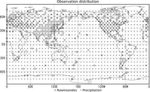
Table 1 The observation errors for the simulated observations

Variables	Observation error
U	1.0 m s^−1
V	1.0 m s^−1
T	1.0 K
Q (specific humidity)	1.0×10^−3 kg kg^−1
Ps (surface pressure)	1.0 hPa
PP (previous 6-h accumulated precipitation)	20% or 50% (in different experiments)

Twenty ensemble members are used in our assimilation experiments. Starting from 1 January 1982, all experiments are initialised with the same initial ensemble created by a random choice of model conditions at an unrelated time in the nature run, so they are very different from the ‘truth’. Observation data are then assimilated into the model with a 6-h cycle. All experiments are run for 1 yr until 1 January 1983. The differences among experiments are summarised in Table 2. First, in ‘RAOBS’, only the rawinsonde observations are assimilated. We denote the control experiment showing the effectiveness of precipitation assimilation as ‘PP_CTRL’, in which precipitation is assimilated, the GT is performed, and the criterion to assimilate precipitation requires at least 10 members of the ensemble (half of the total ensemble size) to have positive precipitation at the analysis grid point (‘10mR’ criterion hereafter). All prognostic variables in the SPEEDY model are updated during the assimilation as in the standard formulation of LETKF. The observation error of precipitation observations in this experiment is rather accurate, 20%, and the localisation length of precipitation observations is the same as RAOBS (i.e. L=500 km). In ‘Qonly’, only the specific humidity Q is updated during the LETKF assimilation of precipitation observations. This is analogous to the conventional ‘nudging’ methods using precipitation observations to only modify the moisture field in the model. The other experiments are as follows: ‘noGT’ does not use the GT; ‘ObsR’ uses the traditional criterion that precipitation is only assimilated when at least a trace of rain (>0.1 mm 6 h⁻¹) is observed. Experiments ‘50%err’ and ‘50%err_noGT’ are conducted to test the impact of lower observation accuracy on the precipitation assimilation, using higher precipitation observation errors of 50% rather than 20%. In addition, several experiments are conducted to test the sensitivity to the criteria for assimilation, and to the localisation lengths of precipitation observations. These are experiments ‘1mR’, ‘5mR’, and ‘15mR’, which vary the critical number of precipitating members in the precipitation assimilation criterion to 1, 5 and 15 from 10 in PP_CTRL, and experiments ‘0.5L’ and ‘0.3L’, which vary the localisation length to 250 and 150 from 500 km in PP_CTRL. Furthermore, for some of the experiments (‘RAOBS’, ‘PP_CTRL’, and ‘Qonly’), we also conduct 5-d free forecasts based on each 6-hourly ensemble mean analysis over the year in order to quantify the forecast impacts of the assimilation of precipitation.

Table 2 Design of all experiments

	Observations
Experiment	Raobs.	Prcp.	Gaussian transf.	Criteria for prcp. assimilation	Obs. error of prcp. obs. (%)	Loc. lengths of prcp. obs.
RAOBS	X
PP_CTRL	X	X	X	Prcp. members≥10	20	1L (=500 km)
Qonly	X	X (only updating Q)	X	Prcp. members≥10	20	1L
noGT	X	X		Prcp. members≥10	20	1L
ObsR	X	X	X	Obs. prcp.>0.1 mm 6h^−1	20	1L
50%err	X	X	X	Prcp. members≥10	50	1L
50%err_noGT	X	X		Prcp. members≥10	50	1L
1mR	X	X	X	Prcp. members≥1	20	1L
5mR	X	X	X	Prcp. members≥5	20	1L
15mR	X	X	X	Prcp. members≥15	20	1L
0.5L	X	X	X	Prcp. members≥10	20	0.5L
0.3L	X	X	X	Prcp. members≥10	20	0.3L

4. Results

4.1. Effect of global precipitation assimilation

Figure 3a shows the evolution of the global root-mean-square (RMS) analysis errors (verified against the nature run) of the u-winds over 1 yr. We only show this variable because the impacts are remarkably similar for all model variables, indicating that the assimilation of precipitation approach is indeed able to influence the full dynamical evolution of the model and not just the moist thermodynamics. Different time intervals are used to show the spin-up stage in the first month and for the remaining 11 months after the spin-up. The average values of RMS analysis errors in the last 11 months are also listed in Table 3. Note that the spin-up takes about 1 month because the ensemble initial states were chosen to be very different from the nature run at the initial time. In the LETKF (or any EnKF) a long spin-up is required in order to estimate not only the truth (with the ensemble mean), but also the ‘errors of the day’ with the ensemble perturbations (Yang et al., 2012).

Fig. 3 The global RMS (a) analysis and (b) forecast errors (verified against the nature run) of u-winds in experiments RAOBS, PP_CTRL, and Qonly. For the analysis errors, the evolution over 1 yr is shown. Different scales on the time axis are used for the spin-up period (the first month) and the remaining 11 months. For the forecast errors, the 11-month (after the spin-up) average values are shown versus the forecast time.

RMS = root-mean-square.

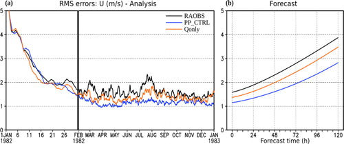
Table 3 Impact of precipitation assimilation on the last 11-month averaged analysis errors of u-wind

	Last 11-month averaged RMSE of U (m s^−1) (percentage changes relative to RAOBS)
Experiments	Globe	NH	TR	SH
RAOBS	1.58	0.67	1.64	2.03
PP_CTRL	1.15 (−27.2%)	0.53 (−20.6%)	1.45 (−11.2%)	0.91 (−55.2%)
Qonly	1.37 (−13.6%)	0.58 (−13.1%)	1.51 (−7.4%)	1.59 (−21.8%)

NH = Northern Hemisphere; SH = Southern Hemisphere; TR = tropics.

It is clear that when all variables (and therefore the full potential vorticity) are modified (PP_CTRL; blue line in Fig. 3a), the improvement introduced by precipitation assimilation is quite large (27.2% reduction in the mean global analysis error) after the first month of spin-up. Not only is the long-term averaged RMS error reduced, but the temporal variation of analysis accuracy is also reduced (e.g. the error jump observed in the RAOBS experiment during July is not seen in PP_CTRL). This result is very encouraging because it clearly shows that assimilating precipitation does bring significant benefits to the LETKF analysis. In contrast, when precipitation observations only modify the moisture field (Qonly; orange line in Fig. 3a), the improvement is much smaller (only 13.6% reduction in the mean global analysis error after the spin-up), even though this approach also uses the GT and the model background-based observation selection criterion of precipitation.

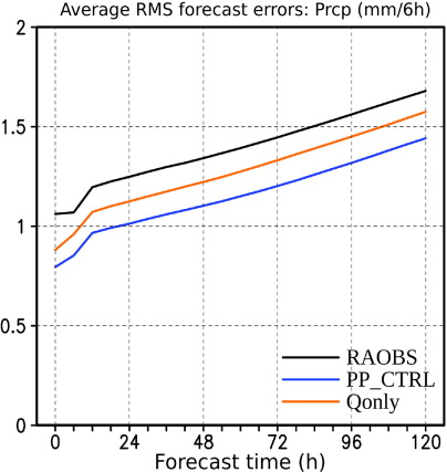
In addition to the LETKF analysis, the impact of precipitation assimilation on model forecasts is also shown on Fig. 3b. The global RMS forecast errors of u-wind are averaged over the last 11 months (i.e. after the spin-up). It is evident that the improvements last throughout the 5-d forecasts, so that the effect of precipitation assimilation is not ‘forgotten’ by the model during the forecast, as experienced with nudging. Contrary to our expectations, the improvement by LETKF modifying only moisture (Qonly) also lasts throughout the forecast, which seems more effective than nudging possibly because of the use of the GT with an EnKF and/or the idealised OSSE framework. However, the improvement in Qonly is much smaller than that in PP_CTRL, and its error growth rate (i.e. the slope) is close to that in RAOBS whereas the error growth rate in PP_CTRL is smaller than for the other two experiments. As indicated before, similar improvements in the analysis and 5-d forecast errors are also observed in all other model variables, including the very important precipitation forecasts. Figure 4 shows that the precipitation forecasts are improved as well by assimilating the precipitation observations. Starting from 12 forecast hours, the error growth rates are stable, and the forecast improvement on precipitation in PP_CTRL relative to RAOBS is more than 2 d.

Fig. 4 As in Fig. 3b, but for precipitation forecast errors.

The effects of GT and the criterion requiring at least 10 members to rain in order to use an observation (10mR) are examined assuming accurate precipitation (20% errors) by comparing the results of PP_CTRL, noGT and ObsR (Fig. 5). As shown in the figure, during the spin-up stage, the LETKF analysis without transforming the precipitation variable (noGT; red line in Fig. 5) is worse than that when the GT is applied. However, with very accurate observations, the GT does not make a significant difference after the spin-up period (Table 4; 26.1% vs. 27.2% reduction in the mean global analysis errors). It is possible that the proposed GT is especially useful to the LETKF assimilation when the model background is less accurate and the difference between model background and the precipitation observations is large. Therefore, when the analysis is accurate enough after the first month of spin-up, the GT does not offer a major advantage. The impact of the GT in experiments with less accurate precipitation observations is, however, much larger as discussed in a later section.

Fig. 5 As in Fig. 3a, but for experiments RAOBS, PP_CTRL, noGT, and ObsR.

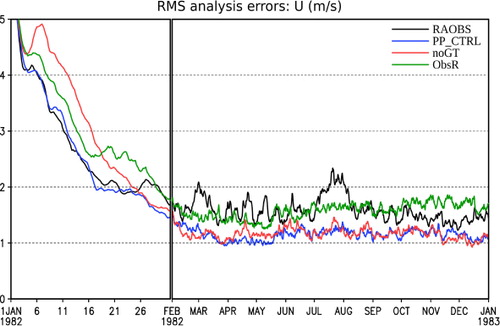
Table 4 Impact of the Gaussian transformation (GT) and accuracy of precipitation observations

	Last 11-month averaged RMSE of U (m s^−1) (percentage changes relative to RAOBS)
Experiments	Globe	NH	TR	SH
RAOBS	1.58	0.67	1.64	2.03
PP_CTRL (20%err)	1.15 (−27.2%)	0.53 (−20.6%)	1.45 (−11.2%)	0.91 (−55.2%)
noGT (20%err)	1.17 (−26.1%)	0.52 (−22.0%)	1.47 (−10.3%)	0.95 (−53.0%)
50%err	1.28 (−19.2%)	0.59 (−12.5%)	1.52 (−6.9%)	1.26 (−38.1%)
50%err_noGT	1.87 (+17.8%)	0.79 (+18.2%)	2.00 (+22.0%)	2.29 (+12.9%)

NH = Northern Hemisphere; SH = Southern Hemisphere; TR = tropics.

In addition, Fig. 5 also shows the impact of the criteria for assimilation of precipitation. We compare the results with the traditional criterion of assimilating only positive rain observations (ObsR) and our newly proposed criterion for assimilating an observation of precipitation that requires at least half of the background members to rain, regardless of whether the observed precipitation is zero or greater than zero (PP_CTRL). The 10mR criterion seems to be essential in order to have effective precipitation assimilation. The analysis of ObsR (green line in Fig. 5), assimilating only positive rain, is obviously degraded from PP_CTRL (Table 5; giving only a 0.3% reduction relative to RAOBS in the mean global analysis error). In particular, the degradation comes mainly from the tropical region (30S–30N; Table 5; 18.7% increase in the mean analysis error), which indicates that this observation-based criterion is not useful in our experimental setup in areas dominated by convective precipitation. Additional experiments with different minimum numbers (1, 5 and 15 out of 20) of precipitating ensemble members required to assimilation precipitation observations are also conducted. As shown in Table 5, with a criterion that is too lenient (requiring only one or five precipitating members), the improvement by precipitation assimilation is also degraded. This indicates that assimilating precipitation observations at locations where precipitating members are rare can hurt the analysis. If stricter criteria (10mR or even 15mR) are used as we do in most experiments in this study, the results are better. Note that this type of criteria also automatically allows some zero-precipitation observations to be assimilated, provided that there are enough precipitating members at the observation location. These locations will probably be in areas of scattered precipitation or near the edges of large-scale precipitation. Average numbers (and percentages) of observations in four different classes in terms of the observation-based criterion and the model background-based criterion in PP_CTRL experiment after the spin-up are shown in Table 6. It is shown that the current 10mR criterion only allows a small portion of the zero-precipitation observations (bold; 48.9 out of 542.6, the average number of zero-precipitation observations) to be assimilated in our control experiment. As the results are significantly improved by using this criterion, it is clear that this small portion of precipitation observations is crucial and really useful in the EnKF data assimilation. Given the fact that the observation data in the upper-right corner of the table (i.e. precipitation observed but no enough precipitating members in the background) are not used in our ‘10mR’ method, and physically this part of data is also expected to have valuable information, it would be worth exploring other ways to exploit information from these data. In our future study with real observations, we will test modifying the criterion so that the observations are also assimilated when precipitation is strong, and at least some ensemble members also show significant precipitation.

Table 5 Impact of assimilation criteria of precipitation observations

	Last 11-month averaged RMSE of U (m s^−1) (percentage changes relative to RAOBS)
Experiments	Globe	NH	TR	SH
RAOBS	1.58	0.67	1.64	2.03
ObsR	1.58 (−0.3%)	0.69 ( +3.4%)	1.94 (+18.7%)	1.40 (−31.0%)
1mR	1.29 (−18.6%)	0.57 (−14.3%)	1.62 (−0.9%)	1.04 (−48.6%)
5mR	1.19 (−25.2%)	0.52 (−22.3%)	1.50 (−8.5%)	0.94 (−53.6%)
PP_CTRL (10mR)	1.15 (−27.2%)	0.53 (−20.6%)	1.45 (−11.2%)	0.91 (−55.2%)
15mR	1.13 (−28.9%)	0.52 (−23.0%)	1.42 (−13.4%)	0.89 (−56.0%)

NH = Northern Hemisphere; SH = Southern Hemisphere; TR = tropics.

Table 6 The average numbers and percentages (in parentheses) of observations in four classes in terms of the observation-based criterion and the model background-based criterion in PP_CTRL experiment after the spin-up

	Observed precipitation rate < 0.1 mm 6 h^−1	Observed precipitation rate ≥ 0.1 mm 6 h^−1
Background precipitation members < 10	493.7 (49.0%)	134.5 (13.3%)
Background precipitation members≥10	48.9 (4.9%)	330.9 (32.8%)

Classes in bold are assimilated into the model and the others are rejected. The total number of observations is 1008 at every cycle.

4.2. Regional dependence

The regional dependence of the impact of precipitation assimilation is considered now. The RMS errors are computed for three regions: the Northern Hemisphere extratropics (30–90N; NH), the tropics (30S–30N; TR), and the Southern Hemisphere extratropics (30–90S; SH). Figure 6 shows the RMS errors of u-wind in 0–5 d forecasts averaged over the last 11 months for main experiments as in Fig. 3b, but shows them for each region. Average RMS analysis errors in the same 11 months in terms of separate regions are also listed in Tables 3–5 and 7 for all experiments.

Fig. 6 As in Fig. 3b, but the RMS forecast errors are calculated separately for the NH extratropics (30–90N; NH), the tropics (30S–30N; TR), and the SH extratropics (30–90S; SH), indicated by different marks on the lines.

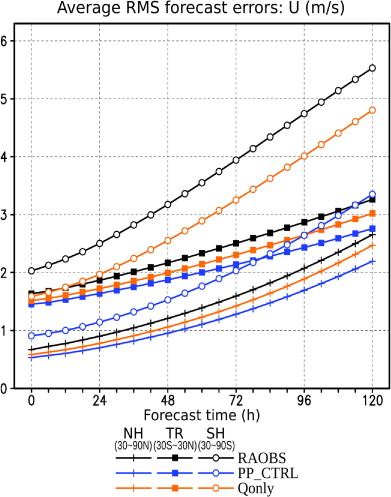
Table 7 Impact of horizontal localization lengths of precipitation observations

	Last 11-month averaged RMSE of U (m s^−1) (percentage changes relative to RAOBS)
Experiments	Globe	NH	TR	SH
RAOBS	1.58	0.67	1.64	2.03
PP_CTRL (1L)	1.15 (−27.2%)	0.53 (−20.6%)	1.45 (−11.2%)	0.91 (−55.2%)
0.5L	1.07 (−32.7%)	0.48 (−28.0%)	1.31 (−20.0%)	0.95 (−53.4%)
0.3L	1.14 (−27.8%)	0.53 (−20.2%)	1.37 (−16.2%)	1.08 (−46.6%)

NH=Northern Hemisphere; SH=Southern Hemisphere; TR=tropics.

It is clear that, as in operational forecasts, these three regions have distinct characteristics of analysis errors, error growth rate and the impact of precipitation assimilation. With only rawinsonde observations (RAOBS), the analysis (0 h) in the NH region is already quite accurate, while the TR analysis is less accurate and the SH analysis is the least accurate. As a result, the precipitation assimilation only has a small effect on the NH region (20.6% reduction in PP_CTRL) but a large effect on the SH region (55.2% reduction in PP_CTRL). The effect on the TR region is even smaller (11.2% reduction in PP_CTRL), which could be due to differences in dynamical instabilities and precipitation mechanisms between the tropical and extratropical regions. The prevailing convective precipitation in the tropics tends to maintain small-scale features and thus would be more difficult to capture in this low-resolution global model implementing only the large-scale mass-flux parameterisation scheme and by low-resolution observations. During the 5-d forecasts, the RMS errors in both NH and SH regions grow with similar rates, faster than that in the TR region, as observed in operational forecasts (Bengtsson et al., 2005), due to the stronger growth rates of mid-latitude baroclinic instabilities. The RMS errors in the NH region are then close to those in the TR region at the end of the 5-d forecasts. The improvement by precipitation assimilation in the SH region is so large that the RMS analysis and most forecast errors in the SH region in PP_CTRL are even better than those in the TR region even though without precipitation assimilation the SH analyses and forecasts are much less accurate. The difference between the LETKF modifying all variables and only modifying moisture is also emphasised in the SH region with the difference in RMSE between Qonly and PP_CTRL increasing with forecast time. Note that in spite of different dynamical nature of error growth in the three regions, precipitation assimilation does lead to positive impacts in all regions.

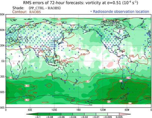
Global maps of (temporally averaged) RMS errors and error reduction of the mid-level vorticity (σ=0.51) for the 72-h forecasts during the last 11 months are shown in Fig. 7. As expected, the error in RAOBS (contours) is large in the SH since the conventional rawinsonde network is quite sparse in that region. The Southern Ocean near the southern end of South America has the largest error in the world presumably because it is the least observed. In contrast, the RAOBS vorticity forecast error is generally small in the NH, especially over the Euro-Asian continent with the densest rawinsonde observations. By including the precipitation observations in LETKF assimilation, the vorticity error reduction (i.e. the RMS error of PP_CTRL – the RMS error of RAOBS; shaded) is large in the SH extratropical region, smaller in the NH extratropical region, and smallest in the tropical region. Once again, the dynamical impact of assimilation of precipitation on the evolution is shown by the fact that the largest error reduction is almost collocated with the regions with the largest error in RAOBS, where the room for improvement is large, and yet the error is still reduced even in rawinsonde-rich NH. The tropical region, instead, shows the smallest improvement, and the eastern equatorial Pacific and the central Africa are the only two areas that show slightly negative impacts. We can conclude that precipitation assimilation in the EnKF has a profound impact on vorticity through the dynamical impact of giving higher weights to the ensemble members with more accurate precipitation. This improvement is observed almost everywhere.

Fig. 7 The global map of RMS 72-h forecast errors of the vorticity at σ=0.51 during the 11 months after the spin-up in RAOBS (brown contour) and the corresponding error reduction from PP_CTRL to RAOBS (shading). The rawinsonde observation locations are also shown in blue open circles.

RMS=root-mean-square.

4.3. Sensitivity to accuracy of the precipitation observations

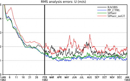
As mentioned in Section 4.1, with accurate precipitation observations of 20%, the application of the GT to the precipitation variable has only a minor impact on the LETKF analysis accuracy after the spin-up (Fig. 5). However, this is not the case when we use more realistic precipitation observation errors of 50%. Figure 8 and Table 4 shows the impact of both larger observation errors as well as the use of the GT. The observation error of precipitation observations is increased to 50% both in the observations and in the LETKF estimation of observation errors. When the GT is used (50%err vs. PP_CTRL which uses 20%err), the analysis becomes only slightly worse (shown as a green line in Fig. 8). However, without the GT and with 50% errors (50%err_noGT; red line in Fig. 8), the precipitation assimilation fails. The LETKF analysis in 50%err_noGT is worse than not assimilating precipitation in each region, as well as globally (Table 4). In other words, without the GT the precipitation assimilation hurts the analysis, whereas 50%err with the GT is almost as good as that obtained with the much smaller 20% errors. This sensitivity test demonstrates the importance of the GT. Less accurate observations will tend to have larger differences from the model background and may not be able to make the analysis accurate enough, so that the non-Gaussian effects become more important for large errors. Note that the errors of real satellite or radar precipitation estimates depend strongly on the degree of spatial and/or temporal averaging applied to the data (Huffman et al., 2007), and that a 50% error in precipitation observations would be considered quite good for such products (Bowman, 2005). Therefore, the GT proposed in this study seems essential for the practical assimilation of precipitation.

Fig. 8 As in Fig. 3a, but for experiments RAOBS, PP_CTRL, 50%err and 50%err_noGT.

4.4. Sensitivity to the localisation lengths of precipitation observations

In all experiments so far, we have used the same horizontal localisation length scale for precipitation assimilation as for rawinsonde observations (500 km, denoted as 1L). As dense global precipitation observations are assimilated in our OSSEs, and precipitation has more local characteristics than the dynamical variables, we speculate that the optimal horizontal localisation length scale for precipitation observations could be smaller than that for rawinsonde observations. Two additional experiments, 0.5L and 0.3L, with 250 and 150 km localisation lengths for precipitation observations, respectively, are conducted. It is observed in Table 7 that the smaller length scales improve the LETKF analyses, and the 0.5L (250 km) length scale would be close to optimal under our current experimental design. The averaged RMS analysis error after the spin-up can be reduced by 32.7% relative to RAOBS when the 0.5L length scale is used, compared with 27.2% when using the original length scale. This suggests that the optimal localisation length could vary with different observation data sets and experimental settings and should be tuned appropriately. It would be interesting to try localisation length scales that vary geographically, for example smaller length in tropics or wherever precipitation is mostly dominated by convection.

5. Conclusions and discussion

Past attempts to assimilate precipitation observations into NWP models have found it difficult to improve model analyses and, especially, model forecasts. In the experience with nudging or variational methods, the forecasts starting from analyses with precipitation assimilation lose their extra skill in forecasts of precipitation or other dynamical variables after a day or less (e.g. Errico et al., 2007). The linear representation of moist physical processes required in the variational data assimilation and the non-Gaussianity of precipitation observations and model perturbations are both major problems in precipitation assimilation (e.g. Bauer et al., 2011).

The EnKF does not require linearisation of the model, thus addressing the first problem. The ensemble can give the ‘error correlation of the day’, essential to produce optimal analyses. In precipitation assimilation, the EnKF can take advantage of the original non-linear precipitation parameterisation to establish useful finite amplitude perturbation covariances between the diagnostic precipitation output and all other state variables without additional computational cost. In this way, the EnKF is expected to more efficiently improve the potential vorticity field compared to nudging or variational approaches. Since potential vorticity is the variable that primarily determines the evolution of the forecast in NWP models, it is not surprising that the analysis improvement due to precipitation used in an EnKF is not so quickly ‘forgotten’ in the forecasts.

In addition to using the EnKF, we introduce two important changes in the data assimilation procedure that contribute to improving the performance of precipitation assimilation. As EnKF (like Kalman filtering) assumes that variables and observations have Gaussian distributions, we first introduce a general algorithm to transform the precipitation variable into Gaussian distribution based on its climatological distribution. To handle the problem that the CDF of precipitation is discontinuous at zero, the middle value (median) of the zero-precipitation cumulative probability is chosen to transform all zero-precipitation values. Second, we propose a forecast-based criterion in the ensemble data assimilation: precipitation observations are assimilated only at grid points where at least some members of the forecast ensemble are precipitating. This automatically allows zero-precipitation observations to be assimilated.

To prove these concepts, we conduct identical-twin OSSEs of global precipitation assimilation with the SPEEDY model and the LETKF. The SPEEDY model is a relatively simple GCM, but able to simulate a realistic climatology (Molteni, 2003). The results in our OSSEs are extremely encouraging. By assimilating global precipitation, the globally averaged RMS analysis errors of u-winds after the spin-up stage are reduced by 27% as compared to only assimilating rawinsonde observations. The improvement is not ‘forgotten’ and persists throughout the entire 5-d forecasts. All model variables show similar impacts of the precipitation assimilation. The improvement is much reduced when only the moisture field is modified by the precipitation observations. By separating the globe into three verification regions, that is the NH extratropics, the tropics, and the SH extratropics, it is shown that the effect of precipitation assimilation is larger in the SH region than that in the NH region since the NH analyses are already accurate due to the denser rawinsonde network. The tropical region shows the least relative improvement probably because of the slower dynamical instabilities and the prevailing convective precipitation type with small-scale features. Reducing the localisation scale in these regions may improve the impact in the tropics.

In addition, a number of comparisons among experiments are made in order to assess the impact of the GT and the observation selection criteria, and the sensitivity to the precipitation error level and to the localisation length scale used for the precipitation observations. Applying the GT does not have a large impact on the analysis errors when precipitation observation errors are at an accurate 20% level, but it is very beneficial when observation errors are at a much higher 50% level. The proposed 10mR data selection criterion (assimilating precipitation at the location where at least half of the members are precipitating) allows using some zero-precipitation observations, and gives much better results than the traditional observation-based criterion of only assimilating positive precipitation, and better than assimilating more observations with a looser criteria (1mR and 5mR criteria).

Although these results are promising, it is important to recognise that the SPEEDY model is simple, that model errors, especially in precipitation parameterisation, are neglected in the current identical-twin OSSE setting, and that the simulated observations might be too idealised. In a real system with model errors, a good precipitation parameterisation scheme would be very important to the precipitation assimilation. We still expect the EnKF to show advantages in this case because the original well-tuned nonlinear moist physics can be directly used for the data assimilation. Besides, the dimensionality of the employed system, a T30 horizontal resolution with seven vertical levels, is very low compared to current operational systems. This low resolution prevents us from addressing some aspects of precipitation assimilation such as the strong and small-scale convective precipitation in tropical regions. In addition, with a real system, the difficulty of estimating errors of precipitation observations will emerge as another critical issue that is absent in the current OSSE framework.

Nevertheless, this study is an essential first step to understand the feasibility and potential of the precipitation assimilation using an ensemble data assimilation method. The results suggest that, in our relatively simple system, the EnKF provides advantages for precipitation assimilation beyond the traditional nudging or variational methods. We plan to carry out follow-up experiments using a more realistic model and assimilating real observations. In the realistic setting, other issues could emerge, such as model errors resulting from the precipitation parameterisation, and the estimation of observation errors including representativeness errors. As precipitation is tightly related to the recent history of moist physics, using a 4D-LETKF that deals with observations at multiple time frames, or some more sophisticated methods such as ‘Running in Place’ (Kalnay and Yang, 2010; Yang et al., 2012), could also be helpful in precipitation assimilation.

Acknowledgements

George Huffman provided invaluable guidance on the characteristics of the satellite precipitation TRMM/TMPA data base. Three reviewers provided valuable comments and suggestions. Reviewer Ross Hoffman made a number of suggestions that helped to improve the manuscript presentation and clarity. This study was partially supported by NASA grants NNX11AH39G, NNX11AL25G, NNX13AG68G and NOAA grants NA100OAR4310248 and CICS-PAEK-LETKF11. The authors gratefully acknowledge support from the Office of Naval Research (ONR) grant N000141010149 under the National Oceanographic Partnership Program (NOPP).

Notes

¹In this study, we define 6-h accumulated precipitation less than 0.1 mm as ‘zero precipitation’.

²In the traditional logarithmic transformation, an arbitrary constant is usually added to the original precipitation value before the transformation, [e.g., ] in order to avoid the singularity at zero precipitation.

³This approach to transforming zero precipitation does not maintain the properties of zero mean and unit standard deviation. However, this does not create problem in the data assimilation because such properties are essentially not required in the climatological distribution.

References

- Bauer P. , Ohring G. , Kummerow C. , Auligne T . Assimilating satellite observations of clouds and precipitation into NWP models. Bull. Am. Meteorol. Soc. 2011; 92: ES25–ES28.
- Bengtsson L. , Hodges K. I. , Froude L. S. R . Global observations and forecast skill. Tellus. A. 2005; 57: 515–527.
- Bocquet M. , Pires C. A. , Wu L . Beyond Gaussian statistical modeling in geophysical data assimilation. Mon. Wea. Rev. 2010; 138: 2997–3023.
- Bowman K. P . Comparison of TRMM precipitation retrievals with rain gauge data from ocean buoys. J. Clim. 2005; 18: 178–190.
- Davolio S. , Buzzi A . A nudging scheme for the assimilation of precipitation data into a mesoscale model. Weather. Forecast. 2004; 19: 855–871.
- Errico R. M. , Bauer P. , Mahfouf J.-F . Issues regarding the assimilation of cloud and precipitation data. J. Atmos. Sci. 2007; 64: 3785–3798.
- Falkovich A. , Kalnay E. , Lord S. , Mathur M. B . A new method of observed rainfall assimilation in forecast models. J. Appl. Meteorol. 2000; 39: 1282–1298.
- Greybush S. J. , Kalnay E. , Miyoshi T. , Ide K. , Hunt B. R . Balance and ensemble Kalman filter localization techniques. Mon. Wea. Rev. 2011; 139: 511–522.
- Hou A. Y. , Skofronick-Jackson G. , Kummerow C. D. , Shepherd J. M . Michaelides S. C . Chapter 6: global precipitation measurement. Precipitation: Advances in Measurement, Estimation and Prediction. 2008; Berlin, Germany. 113–169.
- Hou A. Y. , Zhang S. Q. , Reale O . Variational continuous assimilation of TMI and SSM/I rain rates: impact on GEOS-3 hurricane analyses and forecasts. Mon. Wea. Rev. 2004; 132: 2094–2109.
- Huffman G. J. , Bolvin D. T. , Nelkin E. J. , Wolff D. B. , Adler R. F. , co-authors . The TRMM Multisatellite Precipitation Analysis (TMPA): quasi-global, multiyear, combined-sensor precipitation estimates at fine scales. J. Hydrometeorol. 2007; 8: 38–55.
- Hunt B. R. , Kostelich E. J. , Szunyogh I . Efficient data assimilation for spatiotemporal chaos: a local ensemble transform Kalman filter. Physica. D. 2007; 230: 112–126.
- Jones P. D. , Bradley R. S . Bradley R. S. , Jones P. D . Chapter 13: climatic variations in the longest instrumental records. Climate Since A.D. 1500. 1992; London: Routledge. 246–268.
- Kalnay E. , Yang S.-C . Accelerating the spin-up of ensemble Kalman filtering. Q. J. Roy. Meteorol. Soc. 2010; 136: 1644–1651.
- Koizumi K. , Ishikawa Y. , Tsuyuki T . Assimilation of precipitation data to the JMA mesoscale model with a four-dimensional variational method and its impact on precipitation forecasts. SOLA. 2005; 1: 45–48.
- Kucharski F. , Molteni F. , King M. P. , Farneti R. , Kang I.-S. , co-authors . On the need of intermediate complexity general circulation models: a “SPEEDY” example. Bull. Am. Meteorol. Soc. 2013; 94: 25–30.
- Li X. , Mecikalski J. R . Assimilation of the dual-polarization Doppler radar data for a convective storm with a warm-rain radar forward operator. J. Geophys. Res. 2010; 115: D16208.
- Li X. , Mecikalski J. R . Impact of the dual-polarization Doppler radar data on two convective storms with a warm-rain radar forward operator. Mon. Wea. Rev. 2012; 140: 2147–2167.
- Lopez P . Direct 4D-Var assimilation of NCEP stage IV radar and gauge precipitation data at ECMWF. Mon. Wea. Rev. 2011; 139: 2098–2116.
- Lopez P. , Moreau E . A convection scheme for data assimilation: description and initial tests. Quart. J. Roy. Meteorol. Soc. 2005; 131: 409–436.
- Mesinger F. , DiMego G. , Kalnay E. , Mitchell K. , Shafran P. C. , co-authors . North American regional reanalysis. Bull. Am. Meteorol. Soc. 2006; 87: 343–360.
- Miyoshi T . The Gaussian approach to adaptive covariance inflation and its implementation with the local ensemble transform Kalman filter. Mon. Wea. Rev. 2011; 139: 1519–1535.
- Miyoshi T. , Aranami K . pplying a four-dimensional Local Ensemble Transform Kalman Filter (4D-LETKF) to the JMA Nonhydrostatic Model (NHM). SOLA. 2006; 2: 128–131.
- Molteni . Atmospheric simulations using a GCM with simplified physical parametrizations. I: model climatology and variability in multi-decadal experiments. Clim. Dyn. 2003; 20: 175–191.
- Schöniger A. , Nowak W. , Hendricks Franssen H.-J . Parameter estimation by ensemble Kalman filters with transformed data: approach and application to hydraulic tomography. Water. Resour. Res. 2012; 48: W04502.
- Simon E. , Bertino L . Application of the Gaussian anamorphosis to assimilation in a 3-D coupled physical-ecosystem model of the North Atlantic with the EnKF: a twin experiment. Ocean. Sci. 2009; 5: 495–510.
- Treadon R. E. , Pan H.-L. , Wu W.-S. , Lin Y. , Olson W. S. , co-authors . Global and regional moisture analyses at NCEP. Proceedings of the ECMWF/GEWEX Workshop on Humidity Analysis. 2003; UK, ECMWF: Reading. 33–48.
- Tsuyuki T . Variational data assimilation in the tropics using precipitation data. Part II: 3D model. Mon. Wea. Rev. 1996; 124: 2545–2561.
- Tsuyuki T . Variational data assimilation in the tropics using precipitation data. Part III: assimilation of SSM/I precipitation rates. Mon. Wea. Rev. 1997; 125: 1447–1464.
- Tsuyuki T. , Miyoshi T . Recent progress of data assimilation methods in meteorology. J. Meteorol. Soc. Jpn. 2007; 85B: 331–361.
- Wackernagel H . Multivariate Geostatistics. 2003; Springer, Berlin, Germany. 408.
- Weygandt S. S. , Benjamin S. G. , Smirnova T. G. , Brown J. M . Assimilation of radar reflectivity data using a diabatic digital filter within the Rapid Update Cycle. 12th Conference on IOAS-AOLS. 2008. 88th Annual Meeting, New Orleans, American Meteorological Society. Online at: https://ams.confex.com/ams/88Annual/techprogram/paper_134081.htm .
- Yang S.-C. , Kalnay E. , Hunt B. R . Handling nonlinearity in an ensemble Kalman filter: experiments with the three-variable Lorenz model. Mon. Wea. Rev. 2012; 140: 2628–2646.
- Zhang S. Q. , Zupanski M. , Hou A. Y. , Lin X. , Cheung S. H . Assimilation of precipitation-affected radiances in a cloud-resolving WRF ensemble data assimilation system. Mon. Wea. Rev. 2013; 141: 754–772.
- Zupanski D. , Mesinger F . Four-dimensional variational assimilation of precipitation data. Mon. Wea. Rev. 1995; 123: 1112–1127.
- Zupanski D. , Zhang S. Q. , Zupanski M. , Hou A. Y. , Cheung S. H . A prototype WRF-based ensemble data assimilation system for dynamically downscaling satellite precipitation observations. J. Hydrometeorol. 2011; 12: 118–134.