Observation impact in data assimilation: the effect of non-Gaussian observation error

Abstract

Data assimilation methods which avoid the assumption of Gaussian error statistics are being developed for geoscience applications. We investigate how the relaxation of the Gaussian assumption affects the impact observations have within the assimilation process. The effect of non-Gaussian observation error (described by the likelihood) is compared to previously published work studying the effect of a non-Gaussian prior. The observation impact is measured in three ways: the sensitivity of the analysis to the observations, the mutual information, and the relative entropy. These three measures have all been studied in the case of Gaussian data assimilation and, in this case, have a known analytical form. It is shown that the analysis sensitivity can also be derived analytically when at least one of the prior or likelihood is Gaussian. This derivation shows an interesting asymmetry in the relationship between analysis sensitivity and analysis error covariance when the two different sources of non-Gaussian structure are considered (likelihood vs. prior). This is illustrated for a simple scalar case and used to infer the effect of the non-Gaussian structure on mutual information and relative entropy, which are more natural choices of metric in non-Gaussian data assimilation. It is concluded that approximating non-Gaussian error distributions as Gaussian can give significantly erroneous estimates of observation impact. The degree of the error depends not only on the nature of the non-Gaussian structure, but also on the metric used to measure the observation impact and the source of the non-Gaussian structure.

• mutual information
• relative entropy
• sensitivity

1. Introduction

In assimilating observations with a model, the assumptions made about the distribution of the observation errors are very important. This can be seen objectively by measuring the impact the observations have on updating the estimate of the true state, as given by the data assimilation scheme.

Many data assimilation (DA) schemes are derivable from Bayes’ theorem, which gives the updated estimate of the true state in terms of a probability distribution, p(x|y).1

In the literature, the probability distributions p(y|x), p(x) and p(x|y) are known as the likelihood, prior and posterior, respectively. p(y|x) and p(x) must be known or approximated in order to calculate the posterior distribution, while p(y) is generally treated as a normalisation factor as it is independent of x. The mode of the posterior distribution is then the most likely state given all available information and the mean is the minimum variance estimate of the state.

This paper aims to give insight into how the structure of the given distributions, p(x) and p(y|x), affect the impact the observations have on the posterior, p(x|y). It is known from previous studies that non-Gaussian statistics change the way observations are used in data assimilation (e.g. Bocquet, 2008). This paper presents analytical results to explain this change in observation impact. We begin by presenting the case of Gaussian statistics.

1.1. Gaussian statistics

An often useful approximation for p(y|x) and p(x) is that they are Gaussian distributions, this allows the distributions to be fully characterised by a mean and covariance. The mean of p(y|x) is the value of the observations, y, measuring the true state and the mean of p(x) is our prior estimate of the true state, x _b. The covariances represent the errors in these two estimates of the truth and are given by and for the observations and prior estimate, respectively. In the case when the observations and state are represented in different spaces, it is necessary to transform the likelihood into state space in order to apply Bayes’ theorem. However, if the transform is linear the likelihood continues to be Gaussian in the observed subspace of the state.

In assuming the likelihood and prior (and subsequently posterior) are Gaussian the DA problem is greatly simplified. As such, these assumptions have been used in the development of operational DA schemes for use in numerical weather prediction (NWP). For example, the Gaussian assumption has been used in the development of variational techniques such as 4D-Var used at the Met Office and ECMWF (Rabier et al., 2000; Rawlins et al., 2007), and Kalman Filter techniques such as the ensemble Kalman filter used at Environment Canada (Houtekamer and Mitchell, 1998). In these operational settings, a measure of the impact of observations has been used for

• Improved efficiency of the assimilation by removing observations with a comparatively small impact, e.g. Peckham (1974); Rabier et al. (2002); Rodgers (1996).

• Highlighting erroneous observations or assumed statistics, e.g. Desroziers et al. (2009).

• Improving the accuracy of the analysis by adding observations which should theoretically have a high impact. For example, by defining targeted observations (Palmer et al., 1998) or the design of new observing systems (e.g. Wahba, 1985; Eyre, 1990).

In this work we will concentrate on three measures of observation impact: the sensitivity of the analysis (to be defined) to the observations; mutual information; and relative entropy. Below, these three measures are briefly introduced and interpreted for Gaussian error statistics. For a more in depth study of these measures see relevant chapters within the following books: Cover and Thomas (1991); Rodgers (2000); and Bishop (2006).

1.1.1. The sensitivity of the analysis to the observations.

In Gaussian data assimilation the mode and mean of the posterior distribution are the same and unambiguously define the analysis. In this case the analysis, x _a , is a linear function of the observations and prior estimate:2

where is known as the Kalman gain and is a function of , and . is the observation operator, a (linear) map from state to observation space (See Kalnay, 2003 for an introduction to Gaussian data assimilation.)

The sensitivity of the analysis to the observations has an obvious interpretation in terms of observation impact (Cardinali et al., 2004). It is defined as:3

This is a m×m matrix where m is the size of the observation space.

From eq. (2) we can see that (superscript G refers to the Gaussian assumption) is simply4

The Kalman gain can be written in many different forms including where is the analysis error covariance matrix given by5

Therefore, the sensitivity is inversely proportional to and proportional to . Hence it can be concluded from eqs. (4) and (5), that the analysis has greatest sensitivity to independent observations with the smallest error variance which provide information about the region of state space with the largest prior error.

The diagonal elements of give the self-sensitivities and the off-diagonal elements give the cross-sensitivities. The trace of can be shown to give the degrees of freedom for signal, , that is , where is the i ^th eigenvalue of (Rodgers, 2000).

The analysis sensitivity has proven to be a useful diagnostic of the data assimilation system (Cardinali et al., 2004). It is possible to approximate eq. (4) during each analysis cycle giving a valuable tool for assessing the changing influence of observations and monitoring the validity of the error statistics.

1.1.2. Mutual information.

Mutual information is the change in entropy (uncertainty) when the observations are assimilated (Cover and Thomas, 1991). It is given in terms of the prior, p(x), and posterior, p(x|y), distributions:6

For Gaussian statistics it is unsurprisingly a function of the analysis and background error covariance matrices, and . In this case it is given by7

(Rodgers, 2000), where |*| represents the determinant. As with degrees of freedom for signal, mutual information can be written in terms of the eigenvalues of the sensitivity matrix: . Therefore, the observations which have the greatest contribution to mutual information should also be the observations which the analysis is most sensitive to.

Mutual information has been used in many studies of new observing systems. Eyre (1990) demonstrated its benefits over measuring the change in error variances alone as this measure incorporates information about the change in the covariances too [see eq. (7)].

1.1.3. Relative entropy.

Relative entropy measures the relative uncertainty of the posterior compared to the prior (Cover and Thomas, 1991).8

For Gaussian statistics it is given by9

(see Bishop, 2006). This is the only measure that depends on the value of the analysis, x_a, and so is sensitive not only to how the covariance of the analysis error is affected by the observations but also how the observations affect the actual value of the analysis. Therefore the observations which result in the greatest relative entropy do not necessarily give the largest mutual information or analysis sensitivity if the signal term in eq. (9), , is dominant. However, in a study of the measures, d _s, MI and RE by Xu et al. (2009), it was found that for defining an optimal radar scan configuration the result had little dependence on which of these measures were used.

Relative entropy has received little attention in operational DA due to its dependence on the observation values. However, the shift in the posterior away from the prior, not just the reduction in uncertainty, is clearly an important aspect of observation impact. For this reason, this measure has been included in our current study.

1.2. Non-Gaussian statistics

Although Gaussian data assimilation has proven to be a powerful tool, in some cases a Gaussian distribution gives a poor description of the error distributions. For example, it is found that describing the observation minus background differences (known as innovations) as a Gaussian distribution often underestimates the probability of extreme innovations (the tails are not fat enough) and so the associated observations are assumed to be unlikely rather than providing valuable information about extreme events, and so removed in quality control. Following on from Ingleby and Lorenc (1993), non-Gaussian likelihoods such as the Huber function (Huber, 1973), are being used in operational quality control to make better use of the available observations. Another study of innovation statistics performed by Pires et al. (2010) found significant deviations from Gaussian distributions in the case of quality controlled observations of brightness temperature from the High Resolution Infrared Sounder (HIRS). Pires et al. (2010) concluded that incorrectly assuming Gaussian statistics can have a large impact on the resulting estimate of the state. In this case, the magnitude of the effect on the estimate of the state was seen to depend upon the size of the innovation and the non-Gaussian structure in the likelihood relative to that in the prior.

From eq. (1), we see that there are no restrictions on our choice of p(y|x) or p(x) when calculating the posterior and the more accurately these distributions are defined the more accurate our posterior's representation of our knowledge of the state will be. This simple fact has led to a recent surge in research into non-Gaussian DA methods which are applicable to the geosciences, see van Leeuwen (2009) and Bocquet et al. (2010) for a review of a range of possible techniques.

This work follows on from Fowler and van Leeuwen (2012), in which the effect of a non-Gaussian prior on the impact of observations was studied when the likelihood was restricted to a Gaussian distribution. The main conclusions from that paper are summarised below.

In Fowler and van Leeuwen (2012) a Gaussian mixture was used to describe the prior distribution to allow for a wide range of non-Gaussian distributions. It was shown that, in the scalar case, the sensitivity of the analysis to observations was still given by the analysis error variance divided by the observation error variance as in the Gaussian case [see eq. (4)]. However, the sensitivity could become a strong function of the observation value because the analysis error variance is no longer independent of the observation value. Therefore, when the prior and observation error distributions are fixed but the position of the likelihood, given by the observation value, is allowed to change, the analysis is most sensitive to observations which also result in the largest analysis error variance. This is not a desirable property for a measure of observation impact. Fowler and van Leeuwen (2012) concluded that comparing the analysis sensitivity to the sensitivity when a Gaussian prior was assumed eq. (4), showed that the Gaussian assumption could lead to both a large overestimation and a large underestimation depending on the value of the observation relative to the background and the structure of the prior.

The error in the Gaussian approximation to relative entropy was also seen to give a large range of errors as a function of the observation value relative to the background. However, for a particular realisation of the observation value, the errors in the Gaussian approximation to relative entropy and the Gaussian approximation to the sensitivity did not necessarily agree in sign or magnitude. This highlighted the fact that care is needed when making conclusions about the influence of a non-Gaussian prior on the observation impact.

Mutual information is independent of the realisation of the observation error [as seen in eq. (6)] and so as a measure of the influence of a non-Gaussian prior it provides a more consistent result. Mutual information was also seen in Fowler and van Leeuwen (2012) to be affected a relatively small amount by a non-Gaussian prior.

To summarise: allowing for non-Gaussian prior statistics has a significant effect on the observation impact. The choice of metric is more important than in the Gaussian case as the consistency between the different measures breaks down.

Within this current paper we shall compare these previous findings to the case when it is the likelihood that is non-Gaussian. A non-Gaussian prior or likelihood may result from the properties of the state variable. For example, if the variable has physical bounds then we know, a priori, that the probability of the variable being outside of these bounds is zero which is inconsistent with the infinite support of the Gaussian distribution. This is a particular issue when the variable is close to these bounds. The non-Gaussian prior may also result from a non-linear forecast providing our prior estimate of the state. In this case a wide variety of non-Gaussian distributions are possible and techniques such as the particle filter (van Leeuwen, 2009) allow for the non-linear model to implicitly give the prior distribution. A non-Gaussian likelihood may similarly result from a non-linear map between the observation and state space. However, within this paper we shall only give consideration to linear observation operators. Non-linear observation operators greatly complicate the problem, as not only do they create non-Gaussian likelihoods out of Gaussian observation errors, the structure of the non-Gaussian PDF depends on the value of the observation.

The observation error in this case is defined as:

Possible contributing factors to include:

• Random error associated with the measurement.

• Random errors in the observation operator, for example due to missing processes or linearisation. This is often distinguished from representivity error which deals with the additional error source due to the observations sampling scales which the model is unable to resolve (Janjić and Cohn, 2006).

• Systematic errors are also possible, which may have synoptic, seasonal or diurnal signals some of which can be corrected. There are also gross errors which need to be identified and rejected by quality control (e.g. Gandin et al., 1993; Qin et al., 2010; Dunn et al., 2012).

These sources of random error could all potentially lead to a non-Gaussian structure in the observation errors. Errors associated with the observation operator will in general be state dependent (Janjić and Cohn, 2006). For this reason, within this paper, we will focus on the case of perfect linear observation operators so that the non-Gaussian structure is a characteristic of the instrument error or pre-processing of the observations before they are assimilated. It is assumed that this error source is independent of the state.

In analysing the impact of the non-Gaussian likelihood (rather than a non-Gaussian prior) we shall follow a similar methodology to that in Fowler and van Leeuwen (2012). We shall first derive some general results for the sensitivity of the analysis to the observations. We will then look at a scalar example when the likelihood is described by a Gaussian mixture with two components each with identical variances, GM₂. This will allow for direct comparison to the results in Fowler and van Leeuwen (2012). Finally we will look at the case when the measurement error is described by a Huber function which cannot be described well by the GM₂ distribution.

2. The effect of non-Gaussian statistics on the analysis sensitivity

In non-Gaussian data assimilation the analysis must be explicitly defined. In this work we define the analysis as the posterior mean giving the minimum variance estimate of the state rather than the mode which can be ill-defined when the posterior is multi-modal. In extreme bimodal cases this does lead to the possibility of the analysis having low probability.

The sensitivity of the analysis to the observations can be calculated analytically when either the prior or likelihood is Gaussian, see appendix A. It can be shown that in the case of an arbitrary likelihood and Gaussian prior that the sensitivity is given by10

where µ _a is the analysis (mean of the posterior). When the likelihood is Gaussian, and the expression given in eq. (10) is equal to [see Section 1.1.1, eq. (4)]. However, a non-Gaussian likelihood means that becomes a function of the observation value and hence the sensitivity is also a function of the observation value.

From eq. (10) it is seen that increases as decreases and so for a fixed prior and likelihood structure, the realisation of y for which the analysis has maximum sensitivity also gives the smallest analysis error covariance. In other words, the analysis is most sensitive to observations which improve its accuracy.

This is in contrast to when the prior is non-Gaussian and the likelihood is Gaussian. In this case the sensitivity is given by (see Appendix A)11

This has the same form as eq. (4) in Section 1.1.1. In this case, it is seen that is proportional to the analysis error covariance. Therefore for a fixed prior and likelihood structure, the analysis is most sensitive to observations which reduce its accuracy.

The analysis error covariance is an important aspect in DA in which it is desirable to find a minimum value. Therefore, from eqs. (10) and (11), we can conclude that the influence of a non-Gaussian likelihood on the analysis sensitivity is of a fundamentally different nature to the influence of a non-Gaussian prior. This is demonstrated for a simple scalar example in the next section.

3. A simple example

For comparison to the results in Fowler and van Leeuwen (2012) in which the effect of a skewed and bimodal prior on the observation impact was studied we shall look at the scalar case when the likelihood can be described by a Gaussian mixture with two components each with identical variance, GM₂.12

In this example it is assumed that we have direct observations of the state, x, and so the observation operator, , is simply the identity. From eq. (12) we see that as a function of x, the means of the Gaussian components are and . To ensure that eq. (12) is non-biased, i.e. , we have the constraint , effectively making our observation, y, the mean of the likelihood. This could be restrictive, particularly in the case of a strongly bimodal likelihood when the observation would have a low probability. However, as long as the observation value is chosen to be the likelihood mean plus a constant, the analysis sensitivity presented below remains unchanged.

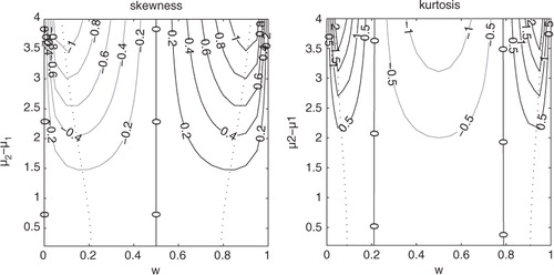
The likelihood in eq. (12) is described by four parameters: the relative weight of the Gaussian components, w, the means of the Gaussian components, µ ₁ and µ ₂, and the variance of the Gaussian components, σ ². These four parameters give rise to a large variety of non-Gaussian distributions, this can be seen from expressions for the skewness and kurtosis.

The variance of the likelihood, p(y|x) as a function of x, is:

Using this expression for the variance we can give the following expression for the skewness of p(y|x):

And the kurtosis of p(y|x):

The values of skewness and kurtosis are plotted in Fig. 1 as a function of w and µ ₂–µ ₁ when σ ²=1. It is clear that for a fixed value of µ ₂–µ ₁, the skewness increases as |w–0.5| increases until it reaches a maximum (indicated by the dotted line in Fig. 1), then the skewness sharply returns to zero as |w–0.5| approaches 0.5 and GM₂ returns to a Gaussian distribution. When the weights are equal (w=0.5) only negative values of kurtosis are possible, increasing as µ ₂–µ ₁ increases. This results in a likelihood with a flatter peak than the Gaussian distribution becoming bimodal as w(1–w)(µ ₁–µ ₂)² exceeds σ ². Positive values of kurtosis are possible when the distribution is also highly skewed. Note that a Gaussian distribution has zero kurtosis.

Fig. 1 Skewness (left) and kurtosis (right) of the GM2 distribution as a function of w and µ ₂–µ ₁ when σ ²=1.

Non-Gaussian structure such as skewness could result from bounds on the observed variable or as a result of non-linear pre-processing. In such a case it should be possible to construct a model of the errors associated with the measurement, such as the GM₂ distribution introduced in this section, through comparison to other observations and prior information for which we have a good estimate of the errors. It is difficult to think of a situation when the likelihood may be strongly bimodal without accounting for a non-linear observation operator. For example, an ambiguity in the observation could result in a bimodal error such as in the use of a scatterometer to measure wind direction from waves (Martin, 2004). Modelling y=|x| results in a likelihood with a GM₂ distribution with equal weights, if the error on the observation, y, is Gaussian. In this case the means of the two Gaussian components would be µ ₁=y and µ ₂=−y. However, the general results provided in Section 2 do not hold. As such in the following analysis the emphasis is not on the extreme bimodal case but the smaller deviations from a Gaussian distribution that the GM₂ distribution allows.

When the prior is given by a Gaussian , the posterior will also be given by a GM₂ distribution [refer to Bayes’ theorem, eq. (1)] with updated parameters. These updated parameters are given by13

where .

for i=1,2.

Note that these have the same form as in Fowler and van Leeuwen (2012) due to the symmetry of Bayes’ theorem.

Given this expression for the posterior distribution we can calculate its mean as: . The sensitivity of the posterior mean to the observations can then be expressed in terms of the parameters of the likelihood distribution as:14

This expression has a striking resemblance to the sensitivity in the case of the non-Gaussian prior, . In eq. (13) of Fowler and van Leeuwen (2012), when the prior has the same form as the likelihood described in eq. (12), was shown to be15

In this case and α_i =((y – μ_i )²)/. Note the distinction between k and ; these parameters are used to define the ratio of the Gaussian variances to the Gaussian component variance for the non-Gaussian likelihood case and the non-Gaussian prior case, respectively.

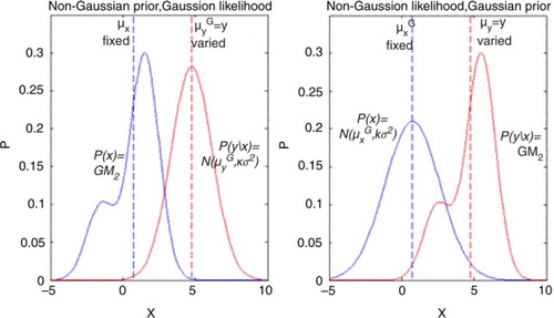
An example of the setup of this simple scalar example is shown in Fig. 2. In the left-hand panel the non-Gaussian prior case which was the focus of Fowler and van Leeuwen (2012) is illustrated and in the right-hand panel the non-Gaussian likelihood case is illustrated. The values of k and have been chosen such that is fixed in the two setups, where is the variance of the likelihood (either Gaussian or not) and is the variance of the prior (which also may or may not be Gaussian).

Fig. 2 Schematic of experimental setup in section 3. Left hand panel: Non-Gaussian prior and Gaussian likelihood as in Fowler and van Leeuwen (2012). Right hand panel: Non-Gaussian likelihood and Gaussian prior, which is the focus of this paper. In each case the non-Gaussian parameters are given by , , . The variance of the Gaussian distributions are chosen such that in each case , for agreement with Fowler and van Leeuwen (2012), giving k=1849/512 and .

We see in eq. (14) that the sensitivity tends towards an upper bound of as the likelihood becomes Gaussian (µ ₁–µ ₂ tends to zero) with no lower bound when the likelihood has two distinct modes (i.e. is large). In contrast, in eq. (15), the sensitivity tends towards a lower bound of as the prior becomes Gaussian with no upper bound when the prior has two distinct modes. The lack of lower and upper bounds for the non-Gaussian likelihood case and non-Gaussian prior case, respectively, has an important consequence for the analysis error variance. From the relationship between the sensitivity and posterior variance given in Section 2 we can conclude that when that and similarly when that . In theory this should never be the case for purely Gaussian data assimilation. The potential for the analysis error variance to be greater than the observation and prior error variances was similarly demonstrated for the case of errors following an exponential law in Talagrand (2003) and when a particle filter is used to assimilate observations with a non-linear model of the Agulhas Current in van Leeuwen (2003).

As a function of the innovation, d=y–µ _x , the shape of is similar to although inverted. In each case the sensitivity is a symmetrical function of d about a central value. In the non-Gaussian likelihood case, this value of d, d ₁, marks a minimum value of . In the non-Gaussian prior case, this value of d, d _p, marks a maximum value of . In general unless all parameters are identical with w=1/2. Away from d ₁ and d _p the sensitivity tends to for the non-Gaussian likelihood case and for the non-Gaussian prior case, as could be expected from the symmetry between k and . When the parameters describing the non-Gaussian distribution are the same, the relative speed at which the sensitivity asymptotes to or depends on the values of k and _, respectively, if then it is the same.

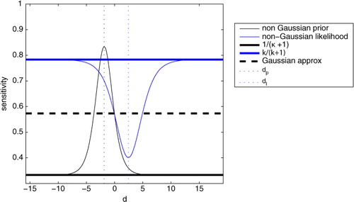
An example of this is shown in Fig. 3, where σ ²=1, w=0.25, µ ₁–µ ₂=3 for both the non-Gaussian likelihood and non-Gaussian prior. for comparison to the example in Fowler and van Leeuwen (2012) and k is chosen to be 1849/512 so that in each case the Gaussian approximation to the sensitivity is the same, that is stays constant even though and are not identical in the two cases, in fact the error variances for the prior and likelihood are larger in the non-Gaussian likelihood case than in the non-Gaussian prior case (see Fig. 2). From eq. (12) and (13) implies that is a broader function of d (thin blue line) than (thin black line) and there is less variance in the sensitivity. This illustrates, that unlike the Gaussian case, the sensitivity is now dependent on the actual values of the error variances rather than just their ratio. The Gaussian approximation to the sensitivity, , is given by the bold dashed line.

Fig. 3 Comparison of as a function of d when the likelihood is non-Gaussian (prior is Gaussian) (thin blue line) and when the prior is non-Gaussian (likelihood is Gaussian) (thin black line). In each case the non-Gaussian distribution is a two component Gaussian mixture with identical variances with parameter values as in Fig. 2. The variance of the Gaussian distributions, also given in Fig. 2, are chosen such that the Gaussian estimate to the sensitivity is the same in each case (bold, dashed line). Also marked on is (bold blue line) and (bold black line), and d _p (black dashed line) and d _l (blue dashed line).

As |d| increases tends to 0/1 in both cases, in effect rejecting one of the modes. In other words the posterior asymptotes to a Gaussian with variance given by in the case of a non-Gaussian likelihood and in the case of a non-Gaussian prior. This explains why the sensitivity, which is given by eq. (10) in the non-Gaussian likelihood case and by eq. (11) in the non-Gaussian prior case, tends to a non-zero constant value as |d| increases. It also explains (with some extra thought) why in the non-Gaussian likelihood case this constant sensitivity is greater than the Gaussian approximation and vice versa when the prior is non-Gaussian.

The value of d, which results in a peak value of , was given in Fowler and van Leeuwen (2012) in terms of the parameters of the non-Gaussian prior.16

We may similarly find an expression for d ₁, which results in a minimum value of , when the likelihood is non-Gaussian. From eq. (10) we know that as the sensitivity increases the analysis error variance decreases. Therefore when the posterior is of the same form as eq. (12), the posterior variance is at a maximum, and hence the sensitivity is at a minimum, when the posterior weights are equal, i.e. the posterior is symmetric. This insight allows us to find the observation value for which the analysis has least sensitivity by finding the d which satisfies .17

Note that in deriving eq. (17) we have made use of the fact that for the terms , w and µ ₁–µ ₂ are considered to be fixed. Therefore we only need to find an expression for µ ₂ which satisfies . This can then be substituted back into the expression for d.

When the weights are equal in the non-Gaussian prior (i.e. ) d _p=0. Similarly when in the non-Gaussian likelihood, . Therefore, when the prior is symmetric but with negative kurtosis the analysis is most sensitive when the mean of the (Gaussian) likelihood is equal to the mean of the prior. Conversely when the likelihood is symmetric but with negative kurtosis the analysis is least sensitive when the mean of the likelihood is equal to the mean of the (Gaussian) prior.

The results illustrated by the example of Fig. 3 can be shown for a range of non-Gaussian distributions described by eq. (12). In Fig. 4, contour plots of (left column) and (right column) are given as a function of d and µ ₂–µ ₁ (top row) and w (bottom row). In all cases k and are varied such that remains the same value as in Fig. 3. In practice this means that as the variance of the non-Gaussian distribution is increased as a result of the parameters describing the distribution changing, the variance of the Gaussian distribution is similarly increased. Indicated in Fig. 4 is the increasing negative kurtosis as increases and the increasing skewness as increases, see Fig. 1 for comparison.

Fig. 4 Comparison of S normalised by its Gaussian approximation when the likelihood is non-Gaussian (prior is Gaussian) (a, c) and when the prior is non-Gaussian (likelihood is Gaussian) (b, d). In the top two panels the effect of separating the Gaussian components (y-axis) is given when the weights are equal. In the bottom two panels the effect of varying the weights of the Gaussian components (y-axis) is given when . In all cases σ ²=1 and is kept constant at by varying the values of k and .

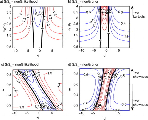
As expected the error in the Gaussian approximation to the sensitivity becomes larger as the skewness and kurtosis of the likelihood/prior increases. The magnitude of the error in the Gaussian approximation to the sensitivity is larger when the prior is non-Gaussian, because in this case leading to a narrower function of sensitivity than when the likelihood is non-Gaussian, as explained previously. If then the error in the Gaussian approximation to the sensitivity would be larger when the likelihood is non-Gaussian. The gradient in the maximum/minimum sensitivity as a function of w (see Figs. 2c and 2d) can be derived from eqs. (16) and (17).

3.1. Comparison of sensitivity to other measures of observation impact

The focus of Fowler and van Leeuwen (2012) was to compare the effect of a non-Gaussian prior on different measures of observation impact. It was seen that like the sensitivity, the error in the Gaussian approximation to relative entropy was a strong function of the innovation. The strong dependence of both the error in the sensitivity and the error in the relative entropy on the innovation means that there is no consensus as to the effect of a non-Gaussian prior on the observation impact for a given observation value. A similar conclusion can be arrived at when the likelihood is non-Gaussian by comparing Figs. 4a and 4c to 5a and 5c, in which fields of and have been plotted, respectively.

Relative entropy [see eq. (8)] is loosely related to the sensitivity in two ways:

(1) As seen when relative entropy was first introduced, relative entropy is dependent on the shift of the posterior distribution away from the prior. The shift of the posterior distribution away from the prior, given by , is proportional to the sensitivity of µ _a to y due to the following relationship:18

  where is an identity matrix of size m (see Appendix A).

  As a function of d, the error in the Gaussian approximation to the shift in the posterior away from the prior will be smallest when . This is only approximate because, unlike in the purely Gaussian case, does not necessarily imply that In Fowler and van Leeuwen (2012) this was wrongly assumed to be true. However, as seen in the example given in Fig. 3, the sensitivities are almost equal to the Gaussian approximation of the sensitivity at d=0. Therefore when , µ _a is very close to µ _x when either the prior or likelihood is non-Gaussian. Away from this the Gaussian approximation will underestimate the shift when it underestimates the sensitivity and similarly overestimate the shift when it overestimates the sensitivity.

(2) Relative entropy also measures the reduction in the uncertainty between the prior and posterior. This is strongly linked to the posterior variance: the larger the posterior variance the smaller the reduction in uncertainty. The sensitivity's relationship to the posterior error variance is given by eqs. (10) and (11). Therefore when the likelihood is non-Gaussian the reduction in uncertainty is overestimated when the sensitivity is overestimated and when the prior is non-Gaussian the reduction in uncertainty is underestimated when the sensitivity is overestimated.

These two comments explain why in Fowler and van Leeuwen (2012) it was found that the error in relative entropy was generally of a smaller magnitude than the error in sensitivity as the two processes above cancel to some degree. It also explains why in this case, when it is the likelihood that it is non-Gaussian, that the error in relative entropy is generally of a greater magnitude than the error in sensitivity as the two processes above reinforce each other to some degree. This can be seen by comparing Figs. 4 and 5.

Fig. 5 As in Fig. 4 but for RE.

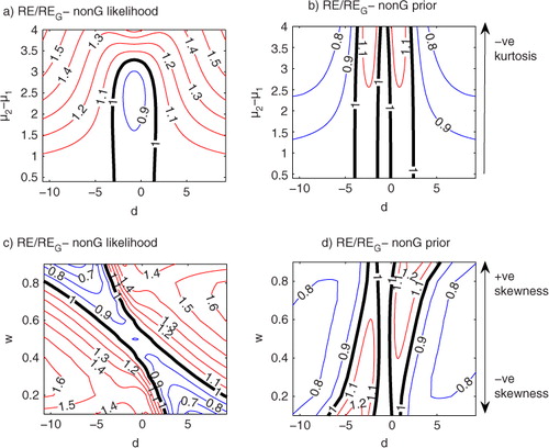
These two comments also explain the asymmetry in the error in relative entropy as a function of d when [see Figs. 5c and 5d]. When the minimum in error in the shift of the posterior at does not coincide with the maximum (minimum) in the reduction in the posterior variance at .

Because of the large variability in the sensitivity and relative entropy as a function of observation value it is useful to look at their averaged values, and . The latter is known as mutual information, a measure of the change in entropy when an observation is assimilated (see Section 1.1.1 and Cover and Thomas, 1991).

On average the Gaussian approximation to the non-Gaussian likelihood underestimates the observation impact [see Figs. 6a and 6c]. This is because the Gaussian estimate of the likelihood underestimates the structure and hence the information in the likelihood. This is analogous to the non-Gaussian prior case presented in Fowler and van Leeuwen (2012) where on average the Gaussian approximation to the non-Gaussian prior overestimated the observation impact due to it underestimating the structure in the prior (see Figs. 6b and 6d).

Fig. 6 Top: Comparison of MI normalised by its Gaussian approximation as a function of w (x axis) and µ ₂–µ ₁ (y axis) when (a) the likelihood is non-Gaussian (prior is Gaussian) and (b) when the prior is non-Gaussian (likelihood is Gaussian). Bottom: Comparison of normalised by its Gaussian approximation as a function of w (x axis) and (y axis) when (c) the likelihood is non-Gaussian (prior is Gaussian) and (d) when the prior is non-Gaussian (likelihood is Gaussian). In all cases σ ²=1 and is kept constant at by varying the values of k and . Red contours indicate values above 1 and blue contours indicate values below one. The contours are separated by increments of 0.02.

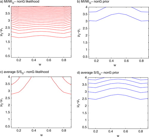
As expected from mutual information's relation to relative entropy and consequently relative entropy's relation to the sensitivity, the error in the Gaussian approximation to MI is greater than the error in the Gaussian approximation to when the true likelihood is non-Gaussian and vice versa when it is the prior that is non-Gaussian.

A summary of some of the key differences between observation impact when the likelihood and prior are non-Gaussian, as discussed in this Section are given in Table 1.

Table 1. Comparison of a non-Gaussian likelihood's and non-Gaussian prior's effect on the observation impact

non-Gaussian likelihood/Gaussian prior	non-Gaussian prior/Gaussian likelihood
in the scalar case.	in the scalar case
Sensitivity is bounded by and 1.	Sensitivity is bounded by 0 and ∞.
As a function of innovation the peak in sensitivity coincides with a minimum in analysis error covariance.	As a function of innovation the peak in sensitivity coincides with a maximum in analysis error covariance.
Variability (as a function of d) in the error of the Gaussian approximation to sensitivity is smaller than the error in the relative entropy.	Variability (as a function of d) in the error of the Gaussian approximation to sensitivity is larger than the error in the relative entropy.
On average Gaussian approximation underestimates observation impact.	On average Gaussian approximation overestimates observation impact.
The error in the Gaussian approximation to the average sensitivity is larger than the error in the Gaussian approximation to mutual information (the average relative entropy).	The error in the Gaussian approximation to the average sensitivity is smaller than the error in the Gaussian approximation to mutual information.

In this section we have studied the observation impact when a non-Gaussian distribution as described by a two-component Gaussian mixture with identical variances, given by eq. (10), is introduced. This has allowed us to understand how the source of non-Gaussian structure affects the different measures of observation impact when the distributions are skewed or have non-zero kurtosis. At the ECMWF, a mixed Gaussian and exponential distribution, known as a Huber function, has recently been introduced to model the observation error for some in-situ measurements (Tavolato and Isaksen, 2009/2010) during quality control. In the next section we will give a brief overview of the observation impact in this specific case.

4. The Huber function

The Huber function has been shown to give a good fit to the observation minus background differences seen in temperature and wind data from sondes, wind profilers, aircrafts, and ships (Tavolato and Isaksen, 2009/2010). From non-Gaussian observation minus background diagnostics it is difficult to derive the observations error structure alone (Pires et al., 2010). However, due to the difficulty in designing a data assimilation scheme around non-Gaussian prior errors, it is a pragmatic choice to assign the non-Gaussian errors to the observations only. The Huber function is described by the following19

where . The distribution is therefore characterised by the following four parameters: y, the observation value, σ ²; the variance of the Gaussian part of the distribution; and the parameters a and b which define the region and the extent of the exponential tails. Therefore as a and b are increased the Huber function relaxes back to a Gaussian distribution.

The Huber function (Huber, 1973), results in a mixture of the l ₂ norm traditionally used in variational data assimilation when the residual, δ, is small (analogous to a Gaussian distribution) and l ₁ norm when the residual is large. Compared to a Gaussian with the same standard deviation this distribution is more peaked and has fatter tails. As such this is poorly represented by the GM₂ distribution. In particular the Huber norm leads to distributions with positive kurtosis values, while the GM₂ distribution can only give negative kurtosis values for a symmetric distribution. As with the GM₂ distribution it is possible to model skewed distributions with the Huber function when .

Despite the differences between the Huber function and GM₂, the same general conclusions already made about observation impact can be applied:

1. The sensitivity can be a strong function of the innovation:

   This is illustrated in Fig. 7. In this example a=−0.5, b=1 and σ ²=2. It is seen that the analysis sensitivity reduces to zero as the observed value gets further from the prior (|d| increases), clear evidence that the Huber function robustly ensures that useful observations contribute to the analysis whilst observations inconsistent with the prior have no impact. This is in contrast to when the likelihood is assumed to be Gaussian and the sensitivity is constant (dashed line). From eq. (8) we can conclude that the peak in sensitivity close to high prior probability coincides with a minimum in the analysis error variance and as |d| increases the analysis error variance tends towards that of the background.

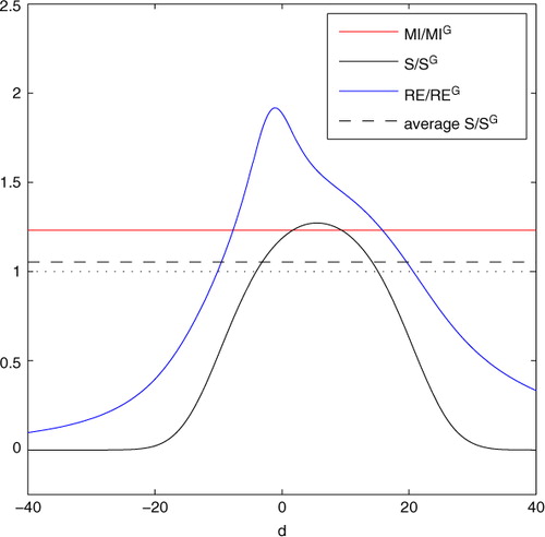
2. The error in the relative entropy assuming a Gaussian likelihood is of a greater magnitude than the error in the sensitivity:

   This is illustrated in Fig. 8. The error in the relative entropy is also asymmetric unlike the error in the sensitivity which is symmetric. This was explained in Section 3.

3. On average the observation impact is underestimated when a Gaussian likelihood is assumed:

   This is also illustrated in Fig. 8. As was seen in the previous section, the Gaussian approximation to mutual information (red) is much poorer that the Gaussian approximation to the averaged sensitivity (black dashed line).

Fig. 7 Left: Huber likelihood (black) , b=1 and σ ²=2, when . Gaussian prior (blue), µ _x =0, variance of prior chosen such that for the variance of the full likelihood ( not σ ²) is 32/43. Right: The sensitivity of the analysis to the observation.

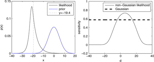
Fig. 8 Mutual information (red), sensitivity (black), relative entropy (blue) and the average sensitivity (black dashed) all normalised by their Gaussian approximations plotted as a function of d.

5. Conclusions and discussion

This work has followed on from the work of Fowler and van Leeuwen (2012), in which the effect of a non-Gaussian prior on observation impact was studied. Here we have compared this to the effect of a non-Gaussian likelihood (non-Gaussian observation error).

There has been much recent research activity in developing non-Gaussian data assimilation methods which are applicable to the Geosciences. It is assumed that by providing a more detailed and accurate description of the error distributions that the information provided by the observations and models will be used in a more optimal way. The aim of this work has been to understand how moving away from the Gaussian assumptions traditionally made in data assimilation will affect the impact that observations have. This analytical study differs from previous studies of observation impact in non-Gaussian DA, such as Bocquet (2008) and Kramer et al. (2012), in which particular case studies were considered.

In Gaussian data assimilation it is known that the impact of observations on the analysis, as measured by the analysis sensitivity to observations and mutual information, can be understood by studying the ratio of to . To use relative entropy to measure the observation impact, it is also necessary to know the values of the observation and the prior estimate of the state. When the assumption of Gaussian statistics are relaxed we have shown that the impact of the observations on the analysis becomes much more complicated and a deeper understanding of the metric used to measure the impact as well as the source of the non-Gaussian structure is necessary.

We have shown that there exists an interesting asymmetry in the relationship of the analysis sensitivity to the analysis error covariance between the two sources of non-Gaussian structure. This means that relaxing the assumption of a Gaussian likelihood has a very different effect on observation impact, as given by this metric, than relaxing the assumption of a Gaussian prior. The sensitivity's dependence upon the analysis error variance only also means that it does not measure the full influence of the observations and may erroneously indicate a degradation of the analysis due to the assimilation of the observations. From this we can conclude that the sensitivity of the analysis to the observations is no longer a useful measure of observation impact when non-Gaussian errors are considered. However the fact that it is possible to derive analytically its relationship with the analysis error covariance, has helped to give us insight into the different effects the two sources of non-Gaussian structure have on relative entropy and mutual information. These measures are much more suitable in the case of non-Gaussian error statistics because they take into account the effect of the observations on the full posterior distribution whilst still having a clear physical interpretation. Mutual information has the added benefit that it is independent of the observation value, and so provides a consistent measure of the observation impact as an experiment is repeated. It is also always positive by construction and so will always measure an improvement in our estimate of the state when observations are assimilated. However, as a consequence mutual information is more difficult to measure in non-Gaussian data assimilation because it involves averaging over observation space.

We have illustrated these findings in the case when the non-Gaussian distribution is modelled by a two component Gaussian mixture. This has allowed for an analytical study of the effect of increasing the skewness and bimodality on observation impact, and has helped to emphasise the differing effect of the source of the non-Gaussian structure on observation impact. The key conclusions from this analytical study have been shown to be applicable to other non-Gaussian distributions such as the Huber function.

The work presented here has been restricted to the case when the map between observation and state space is linear. However, there are many observation types which are not linearly related to state variables, for example, satellite radiances are a non-linear function of temperature, humidity, etc., throughout the depth of the atmosphere. In this case, even if the observation error were Gaussian, a non-linear observation operator would result in a non-Gaussian likelihood in state space. The results shown in this paper are not directly applicable to this source of non-Gaussianity, as the structure of the likelihood function in state space is now dependent on the observation value. This makes an analytical study much more difficult as shown in appendix A.3. A study of the effect of a non-linear observation operator is left for future work.

6. Acknowledgements

This work has been funded by the National Centre for Earth Observation (NCEO) part of the Natural Environment Research Council (NERC), project code H5043718, and forms part of the ‘ESA Advanced Data Assimilation Methods’ project, contract number ESRIN 4000105001/11/I-LG. We would also like to thank Carlos Pires and two anonymous reviewers for their valuable comments.

7. Appendix

A.1. The sensitivity of the analysis mean to the likelihood mean

Bayes’ theorem states that the probability of the state, x, given information y can be derived from the prior probability of x and the likelihood.20

where .

The analysis can be given by the mean of the posterior,21

Substituting eqs. (20) into (21) we see that the analysis is only dependent on the observation value through the likelihood, p(y|x). The sensitivity of the analysis in observation space to the observation value, , is then given by22

Recall that is the (linear) operator which transforms a vector from state to observation space.

It is also of interest to look at the sensitivity of the analysis to the mean of the prior, , in observation space. In this case it is only the prior, p(x), in eq. (20) which is sensitive to and so the sensitivity of the analysis to the mean of the prior is given by23

In the following subsections we will show that it is possible to evaluate these sensitivities when either the prior or likelihood are Gaussian.

A.2. Non-Gaussian prior, Gaussian likelihood

Let p(x) be arbitrary and p(y|x) be Gaussian with mean and error covariance .24

Here m is the size of observation space. Therefore25

A.2.1. Analysis sensitivity to observations.

Equation (25) can be substituted into eq. (22) to give26

Note that is the analysis error covariance matrix, . eq. (26) therefore simplifies to27

A.2.2. Analysis sensitivity to background.

In calculating the sensitivity with respect to the background (the mean of the prior), in this case, we do not have access to . However we do know as the change in the probability caused by perturbing the value of x is the same as perturbing by the same magnitude but in the opposite direction. Therefore we can utilise integration by parts, that is, .

First evaluate the first term of eq. (23):

Let and . Therefore . v can be found by noting , it then follows that .28

The first term of eq. (23) is then29

Likewise we may evaluate the second term of eq. (23):

Let and again. Therefore and v is unchanged.30

The second term of eq. (23) is then31

It then follows that32

A.3. Non-Gaussian likelihood, Gaussian prior

Let p(y|x) be arbitrary and p(x) be Gaussian with mean and error covariance .33

Therefore34

A.3.1. Analysis sensitivity to observations.

The derivation of is analogous to the derivation of in the previous section, as in this case is unknown and so we must make use of integration by parts.

It can be shown that in this case35

A.3.2. Analysis sensitivity to background.

The derivation of is analogous to the derivations of in the previous section as in this case is known.36

From this we can conclude that when either the prior or likelihood is Gaussian it is always the case that:37

A.4. Non-linear observation operator

Following a similar methodology as in Appendix A.2 and A.3, the analysis sensitivity to the observations when the observation operator is non-linear, represented by h(x), can be shown to be38

where is the observation operator linearised about the analysis. In this expression it has been assumed that the likelihood in observation space is Gaussian, i.e. but no assumptions about the prior have been necessary. When h(x) is non-linear there is no longer a clear relationship between the sensitivity and the analysis error covariance matrix.

References

- Bishop C . Pattern Recognition and Machine Learning. 2006; Springer Science+Business Media, LLC, New York.
- Bocquet M . Inverse modelling of atmospheric tracers: non-gaussian methods and second-order sensitivity analysis. Nonlinear Process. Geophys. 2008; 15: 127–143.
- Bocquet M , Pires C. A , Wu L . Beyond gaussian statistical modeling in geophysical data assimilation. Mon. Wea. Rev. 2010; 138: 2997–3023.
- Cardinali C , Pezzulli S , Andersson E . Influence-matrix diagnostics of a data assimilation system. Q. J. Roy. Meteorol. Soc. 2004; 130: 2767–2786.
- Cover T. M , Thomas J. A . Elements of Information Theory (Wiley Series in Telecommunications). 1991; John Wiley, New York.
- Desroziers G , Berre L , Chabot V , Chapnik B . A posteriori diagnostics in an ensemble of perturbed analyses. Mon. Wea. Rev. 2009; 137: 3420–3436.
- Dunn R. H. J , Willet K. M , Thorne P. W , Woolley E. V , Durre I , co-authors . HadISD: a quality-controlled global synoptic report database for selected variables at long-term stations from 1973–2011. Clim. Past. 2012; 8: 1649–1679.
- Eyre J. E . The information content of data from satellite sounding systems: a simulation study. Q. J. Roy. Meteorol. Soc. 1990; 116: 401–434.
- Fowler A. M , van Leeuwen P. J . Measures of observation impact in non-gaussian data assimilation. Tellus. 2012; 64: 17192.
- Gandin L. S , Monrone L. L , Collins W. G . Two years of operational comprehensive hydrostatic quality control at the national meteorological center. Weather. Forecast. 1993; 57: 57–72.
- Houtekamer P. L , Mitchell H. L . Data assimilation using an ensemble kalman filter technique. Mon. Wea. Rev. 1998; 126: 798–811.
- Huber P. J . Robust regression: asymptotics, conjectures, and monte carlo. Ann. Stat. 1973; 1: 799–821.
- Ingleby B , Lorenc A . Bayesian quality control using multivariate normal distributions. Q. J. Roy. Meteorol. Soc. 1993; 119: 1195–1225.
- Janjić T , Cohn S . Treatment of observation error due to unresolved scales in atmospheric data assimilation. Mon. Wea. Rev. 2006; 134: 2900–2915.
- Kalnay E . Atmospheric Modeling, Data Assimilation and Predictability. 2003; Cambridge University Press, New York.
- Kramer W , Dijkstra H. A , Pierini S , van Leeuwen P. J . Measuring the impact of observations on the predictability of the kuroshio extension in a shallow-water model. J. Phys. Oceanogr. 2012; 42: 3–17.
- Martin S . An Introduction to Ocean Remote Sensing. 2004; Cambridge University Press, Cambridge.
- Palmer T. N , Gelaro R , Barkmeijer J , Buizza R . Singular vectors, metric, and adaptive observations. J. Atmos. Sci. 1998; 55: 633–653.
- Peckham G . The information content of remote measurements of the atmospheric temperature by satellite ir radiometry and optimum radiometer configurations. Q. J. Roy. Meteorol. Soc. 1974; 100: 406–419.
- Pires C. A , Talagrand O , Bocquet M . Diagnosis and impacts of non-gaussianity of innovations in data assimilation. Pysica. D. 2010; 239: 1701–1717.
- Qin Z.-K , Zou X , Li G , Ma X.-L . Quality control of surface station temperature data with non-gaussian observation-minus-background distributions. J. Geophys. Res. 2010; 115
- Rabier F , Fourrié N , Chafai D , Prunet P . Channel selection methods for infrared atmospheric sounding interferometer radiances. Q. J. Roy. Meteorol. Soc. 2002; 128: 1011–1027.
- Rabier F , Jarvinen H , Klinker E , Mahfouf J.-F , Simmons A . The ECMWF operational implementation of four-dimensional variational data assimilation. I: experimental results and simplified physics. Q. J. Roy. Meteorol. Soc. 2000; 126: 1143–1170.
- Rawlins F , Ballard S. P , Bovis K. J , Clayton A. M , Li D , co-authors . The Met Office global four-dimensional variational data assimilation scheme. Q. J. Roy. Meteorol. Soc. 2007; 133: 347–362.
- Rodgers C. D . Information content and optimisation of high spectral resolution measurements. Proc. SPIE. 1996; 2830: 136–147.
- Rodgers C. D . Inverse Methods for Atmospheric Sounding. 2000; World Scientific, Singapore.
- Talagrand O . Bayesian Estimation. Optimal Interpolation. Statistical Linear Estimation in Data Assimilation for the Earth System, Volume 26 of NATO Science Series IV Earth and Environmental Sciences. 2003; , Netherlands: Springer.
- Tavolato C , Isaksen L . Huber norm quality control in the IFS. ECMWF Newsletter No. 122, 2009/2010.
- van Leeuwen P. J . A variance-minimizing filter for large-scale applications. Mon. Wea. Rev. 2003; 131: 2071–2084.
- van Leeuwen P. J . Particle filtering in geophysical systems. Mon. Wea. Rev. 2009; 137: 4089–4114.
- Wahba G . Design criteria and eigensequence plots for satellite-computed tomography. J. Atmos. Oceanic. Technol. 1985; 2: 125–132.
- Xu Q , Wei L , Healy S . Measuring information content from observations for data assimilation: connection between different measures and application to radar scan design. Tellus. 2009; 61A: 144–153.