Calibrating ensemble reliability whilst preserving spatial structure

Abstract

Ensemble forecasts aim to improve decision-making by predicting a set of possible outcomes. Ideally, these would provide probabilities which are both sharp and reliable. In practice, the models, data assimilation and ensemble perturbation systems are all imperfect, leading to deficiencies in the predicted probabilities. This paper presents an ensemble post-processing scheme which directly targets local reliability, calibrating both climatology and ensemble dispersion in one coherent operation. It makes minimal assumptions about the underlying statistical distributions, aiming to extract as much information as possible from the original dynamic forecasts and support statistically awkward variables such as precipitation. The output is a set of ensemble members preserving the spatial, temporal and inter-variable structure from the raw forecasts, which should be beneficial to downstream applications such as hydrological models. The calibration is tested on three leading 15-d ensemble systems, and their aggregation into a simple multimodel ensemble. Results are presented for 12 h, 1° scale over Europe for a range of surface variables, including precipitation. The scheme is very effective at removing unreliability from the raw forecasts, whilst generally preserving or improving statistical resolution. In most cases, these benefits extend to the rarest events at each location within the 2-yr verification period. The reliability and resolution are generally equivalent or superior to those achieved using a Local Quantile-Quantile Transform, an established calibration method which generalises bias correction. The value of preserving spatial structure is demonstrated by the fact that 3×3 averages derived from grid-scale precipitation calibration perform almost as well as direct calibration at 3×3 scale, and much better than a similar test neglecting the spatial relationships. Some remaining issues are discussed regarding the finite size of the output ensemble, variables such as sea-level pressure which are very reliable to start with, and the best way to handle derived variables such as dewpoint depression.

• Brier Skill Score
• climatological thresholds
• Ensemble Copula Coupling
• Local Quantile-Quantile Transform
• medium range
• multimodel ensemble
• rank histogram
• TIGGE

1. Introduction

Ensemble weather forecasts aim to improve decision-making by predicting the probability of each possible outcome. The quality of a probabilistic forecast can be split into two key attributes: First, the probabilities should be statistically reliable in the sense that an event assigned probability p should occur in a fraction p of such cases. This allows users to obtain the maximum benefit by acting when the forecast probability exceeds the ratio of the cost of taking action to the loss it would prevent (Richardson, 2000). Second, the ensemble should provide as much discrimination as possible between situations in which the event is more or less likely. This statistical resolution ensures the forecasts provide more information than always forecasting a probability equal to the climatological frequency of the event (which would be perfectly reliable). Measures of forecast performance such as the Brier Skill Score (BSS) can be decomposed in this way (Wilks, 2006).

Real forecasting systems run in constrained time with finite computing resources and imperfect models, observations, boundary conditions, data assimilation and perturbation schemes. These limit their fundamental ability to distinguish whether or not an event will occur. They also limit the statistical reliability of the forecast probabilities. Statistical calibration schemes use historic measurements of forecast performance to make adjustments which aim to improve upon the raw forecasts. One might expect limited scope for improving statistical resolution, since the calibration cannot introduce case-specific information that is not contained in the underlying forecast. However, the training data can provide a mapping from raw probabilities to actual observed frequencies, so one might hope to significantly reduce statistical unreliability whilst also preserving the resolution of the raw forecasts. This is the core aim of the calibration work presented in this paper.

A variety of ensemble calibration methods have been proposed in the literature. Examples include simple bias correction (e.g. Johnson and Swinbank, 2009), more detailed quantile mapping (Bremnes, 2007), inflation (Johnson and Swinbank, 2009; Flowerdew and Bowler, 2011), nearby locations and thresholds (Atger, 2001), direct mapping of forecast probabilities to past observed frequencies (Primo et al., 2009), forecast assimilation (Coelho et al., 2006), methods such as Bayesian Model Averaging (Raftery et al., 2005, Fraley et al., 2010) that dress each ensemble member with a kernel, methods such as Non-homogeneous Gaussian regression (NGR; Gneiting et al., 2005, Hagedorn et al., 2008) and logistic regression (Hamill et al., 2008; Wilks, 2009) that map raw forecast quantities to parameters of a fixed output distribution, analogue methods (Hamill and Whitaker, 2006; Stensrud and Yussouf, 2007) and neural networks. Applequist et al. (2002) compares a variety of similar methods applied to deterministic input. The various approaches differ in the properties targeted (bias, climatology, spread, reliability, …), the predictors used (ensemble members, raw probabilities, ensemble mean/spread, …), the form of the output (ensemble members, probabilities to exceed specific thresholds, a parameterised probability distribution, …), the extent of the training required (a few recent days/weeks through to years of reforecasts), and whether the method attempts to add high-resolution detail to low-resolution input.

Precipitation highlights a number of issues which need to be addressed by a generic calibration scheme. It has an awkward distribution, which is skewed, cannot be negative, and includes finite probability of zero precipitation. This last point prevents any direct transformation of precipitation into a Gaussian variable. Simple methods such as bias correction and perturbation scaling are also awkward to apply to variables with these characteristics.

Most calibration methods focus on one output at a time, without considering spatial, temporal, or inter-variable relationships. However, these relationships are required to produce fields and timeseries which are physically realistic, and to support the use of calibrated data in downstream systems. A hydrological model, for instance, depends on space–time integrals of rainfall, and its relationship to variables such as temperature. The importance of spatial relationships is particularly obvious when trying, as here, to apply calibration to gridded data, as opposed to predictions for a set of discrete sites.

This paper presents a calibration method that directly targets the statistical reliability of the forecast probabilities. This should implicitly calibrate both climatology and spread, since these involve integrals of the case-specific probability distributions. The scheme was originally developed for precipitation (Flowerdew, 2012), and makes minimal assumptions about the underlying statistical distributions. Instead, it tries to extract as much information as possible from the original dynamic ensemble forecasts. The implied probability distribution is mapped back onto the original ensemble in order to preserve its spatial, temporal and inter-variable structure. The net effect is to slightly adjust the original ensemble members so that the probabilities become statistically reliable. The present paper examines the extent to which this general approach is effective for a wider range of surface variables, including temperature, wind speed, pressure and dewpoint depression. It considers a wider European area than was possible with the UK-focussed dataset used in Flowerdew (2012), and explores performance for more extreme thresholds. Whilst reliability calibration (Primo et al., 2009) and the ensemble reconstruction method (Bremnes, 2007; Schefzik et al., 2013) have been considered by previous authors, the particular combination, the binned approach to reliability calibration, the way in which training data are aggregated over space, and the details of the verification all appear to be novel.

The rest of this paper is laid out as follows. Section 2 describes the reliability calibration method, and a generalised bias correction against which it is compared. Section 3 describes the forecast and observation data used to train and test the calibration schemes. The results are shown in section 4, including performance for moderate and more extreme thresholds, as well as the impact on spatial averages and a derived variable. Conclusions and suggestions for future work are given in section 5.

2. Calibration methods

This section describes the two calibration methods which are tested in this paper. The main reliability calibration method is presented in section 2.2. Before this, section 2.1 introduces a simpler, established method for mapping between the forecast and observed climatologies. This is used as a benchmark to ensure the reliability-based approach is competitive. The circumstances in which climatology calibration is more or less successful also help to illustrate the relative importance of biases as compared to other systematic errors in different situations. Some common issues regarding the organisation of training data are discussed in section 2.3.

2.1. Climatology calibration

One of the most basic systematic errors which a calibration scheme might attempt to correct is consistent over- or under-prediction of the observed value. For unbounded variables like temperature, one might simply consider the overall mean difference between forecast and observations (bias), as in Johnson and Swinbank (2009). For bounded variables such as precipitation, more elaborate approaches are needed to avoid unphysical negative values and leave finite probability at zero precipitation rather than some other value. More generally, there is no guarantee that the same shift is appropriate for all forecast values; indeed comparison of forecast and observed climatology along the lines of Flowerdew (2012) shows different offsets for different quantiles.

One could attempt to solve this problem by conditioning the bias on ranges of the forecast value. However, this convolves true bias with forecast uncertainty, due to the ‘regression to the mean’ effect. A more satisfactory non-parametric approach is to match quantiles of the forecast and observed climatology. This simply assumes that they should represent the same set of physical states and the mapping should be monotonic. If the 95th percentile of 12 h precipitation from the model was 6.2 mm, forecasts of 6.2 mm would be mapped to the corresponding quantile from observations, which might be 6.8 mm. This principle is known as the Local Quantile-Quantile Transform (Bremnes, 2007).

The specific ‘climatology calibration’ tested below is implemented as follows, based on a year of training data. Whilst this will not be enough to accurately estimate the outer quantiles of long-term climatology, it is hoped that the model and observations represent sufficiently similar sub-climatologies driven by the boundary conditions affecting this matched period that the mapping from forecast to observed values can be recovered. The training data is divided into 3-month blocks. Within each block, the 1,3,5,10,…,90,95,97,99th percentiles of the (2n+1)²-gridpoint domain around each gridpoint are identified, separately for each data source and lead time. The quantity n is referred to as the degree of spatial padding, and its optimal value is probed by the tests presented in section 4.3 below. It is important that the forecast climatologies be restricted to observed points, particularly with larger values of n. This ensures that results near the edges of the observation domain represent the same set of locations. On the other hand, no attempt is made to exclude forecast dates which lack corresponding observations, since these should not introduce any systematic difference in climatology, and one does not expect forecasts at longer lead times to precisely match the timing of observed events.

The final calibration at each gridpoint is based on the mean over the four 3-month blocks of the local quantile values. An average of 3-month quantiles was chosen over 12-month quantiles to make the result equally applicable to all seasons and avoid the sampling noise that might otherwise arise from results being dominated by the most extreme seasons. The forecast values are calibrated by linear interpolation/extrapolation between the matching percentiles of forecast and observed climatology [in the language of eq. (1) below, if these climatologies are given by vectors C _f and C _o respectively, and x is the raw forecast value, then the calibrated value is L(C _o ,C _f ,x)]. The percentile spacings were chosen to explore the resolved shape of the climatology mapping, whilst hopefully limiting noise sufficiently that extrapolation at the extremes remains plausible.

2.2. Reliability calibration

The reliability calibration scheme, which forms the main focus of this paper, is illustrated in Fig. 1. It consists of a series of steps which are described in the following subsections.

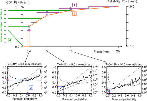
Fig. 1 An illustration of how the reliability calibration method modifies one gridpoint from a single forecast source. (1) The raw ensemble members imply a cumulative density function (CDF; stepped line in upper half). The training (lower half) provides reliability (solid) and sample count (dashed, using the logarithmic scale to the right of each subplot) for this forecast source against a fixed set of thresholds. (2) This allows the raw probability at each threshold (purple circles) to be mapped to the corresponding observed frequency (red crosses), as indicated by the blue arrows within each reliability diagram. (3) Replicated in the upper half of the diagram, these results form a calibrated CDF (red). Note the opposite sense in which reliability diagrams (probability to exceed a threshold) and CDFs (probability to be less than or equal to a threshold) are traditionally defined. (4) New members (green horizontal lines at top left) are assigned to equally divide the probability range, in the same order as the raw ensemble members.

2.2.1. Accumulation of training data.

The core of the calibration scheme constructs a series of mappings from raw forecast probability to observed event frequency, for a set of pre-specified thresholds appropriate to each variable. The criteria for choosing these thresholds are discussed in section 2.2.5 below. The training accumulates the sample count, mean forecast probability and observed event frequency for each gridpoint, lead time, threshold, and forecast probability bin. Splitting the training data by location and forecast probability provides a more situation-specific calibration. However, if the individual sample counts become too small, the adjustments will contain more noise than signal and thus make the forecasts worse rather than better. To reduce both statistical noise and memory usage, the standard configuration uses just five probability bins: three across the main probability range and one each for cases where zero or all members exceed the threshold. This partition was motivated by the observation that most reliability diagrams (including those shown in Fig. 1) are near-linear across the main probability range, but sometimes show jumps for the case where zero or all members forecast the event. This is particularly common at short lead times, presumably arising from underspread. Early tests showed a small benefit of this arrangement compared to five equally-spaced probability bins.

The reliability calibration scheme attempts to balance the remaining statistical noise against the locality of the training data through a procedure of dynamic spatial aggregation. The final statistics for each probability bin of each threshold are averaged over a square domain centred on each gridpoint, which is made just large enough to provide at least 200 cases where the forecast probability fell within that bin. This means that common situations are trained on locally relevant data, whilst rare situations draw data from a wider area, since a bland but relatively noise-free adjustment is much better than a local but noisy one. The standard configuration allows the use of data up to 20° away. Bins with fewer than 200 samples at the maximum padding are discarded (an improved scheme might combine them with neighbouring probability bins). The 20° limit was introduced out of concern that training which was too non-local might be detrimental. In most cases tested, the move from 20° to whole-domain maximum padding has little impact other than to increase the computational cost.

For n independent samples, the number of times an event with underlying probability φ would be observed follows a binomial distribution with variance nφ(1-φ). Expressed as a fraction of the expected number of events (nφ), the standard error is therefore . 200 samples thus give about a 7% error on φ=0.5 and a 20% error on φ=0.1, rising to as φ→0. A more elaborate scheme focussed on equalising the fractional error in the calibrated probabilities might derive the minimum sample count as a function of the forecast probability or observed event frequency.

Aside from locality, the spatial aggregation procedure takes no account of gridbox characteristics such as orography or whether they lie over land or sea. A more elaborate scheme might generalise the spatial distance to a gridbox similarity index that included such factors. Calibration would then be based on the most similar locations consistent with the required sample count, rather than relying on distance alone. Hamill et al. (2008) suggest some criteria for identifying ‘similar’ locations.

2.2.2. Calibrating univariate reliability.

Having obtained the spatially-aggregated training data, the calibration of the target forecast proceeds as follows. For each threshold, gridpoint and lead time, the training provides vectors S and R, respectively, giving the mean forecast probability and observed event frequency in bins defined by the forecast probability. This reliability diagram provides the required mapping from raw forecast probability to the actual frequency with which the event occurred in the training sample when that probability was forecast, as illustrated by the blue arrows inside the lower panels of Fig. 1. The raw probability, p, from the target forecast is calculated as the fraction of members which exceed the threshold. Where this coincides exactly with an element of S, the calibrated probability is just the corresponding element of R. Probabilities between and beyond the mean values in S are handled using interpolation/extrapolation, taking a linear approach for simplicity:1

The subscripts l and h denote the low and high bin indices upon which the interpolation/extrapolation is based. Where possible, these will be chosen so that S _l is the nearest available value below p and S _h the nearest larger value. Where extrapolation is required, the two bins with mean forecast probability closest to p (on whichever side) will be used, and the resulting probability capped at 0 or 1 if required. Where only one bin exceeded the minimum sample count, is simply set to that observed (approximately climatological) event frequency. For locations with insufficient observations to reach the minimum sample count in any bin, no calibrated forecast is produced.

Since each calibrated probability is based on observed event frequencies, the result should be reliable by construction, within the limits of stationarity and statistical noise. If the calibration process stopped at this point, one could produce maps of calibrated probabilities to exceed the pre-defined thresholds, but there would be no direct information on individual member values or spatial relationships.

2.2.3. Formation of calibrated CDF.

The rest of the process regards these calibrated probabilities as providing a calibrated cumulative density function (CDF) for each gridpoint and lead time. This is represented by the red line in the upper half of Fig. 1. Since each threshold is calibrated with a different set of predictors, it is possible for the calibrated probabilities to be non-monotonic as a function of threshold. In practice, the scheme appears to have sufficient control over statistical noise that this effect is small (with a mean probability decrease of about 0.015 across the approximately 5% of cases which were affected in early tests on precipitation). The current implementation sorts the probabilities to force them to be monotonic, though the detailed treatment seems to have negligible impact on probabilistic scores. This gives a vector of probabilities corresponding to the vector of training thresholds T.

2.2.4. Mapping back to ensemble members.

The next step identifies a set of ensemble member values to represent the calibrated CDF. These are chosen to lie at the series of quantiles, q, that divide the CDF into blocks of equal probability, following the theory behind rank histograms (Hamill and Colucci, 1997):2

where N is the number of ensemble members. These quantiles are marked by the green horizontal lines at the top left of Fig. 1. The corresponding forecast values, , are obtained by linear interpolation between the calibrated thresholds:3

using the formula, L, defined in eq. (1). This is indicated by where the green arrows meet the red line in Fig. 1. To provide a clean distinction between zero and non-zero precipitation, all results below the lowest threshold are mapped to zero for this variable. To close the remaining ends of the distribution, the cumulative probability is set to 0 or 1 as appropriate at outer boundaries which are pre-defined for each variable, and listed in Table 1 below. A more elaborate scheme might fit an extreme value distribution to close these ends of the CDF (e.g. Ferro, 2007).

Table 1. The number (nThresh) and values of the training thresholds, and the output value ranges used by the reliability calibration scheme for each variable considered in this paper

Variable	nThresh	Training thresholds	Value range	Units
12 h-accumulated precipitation	12	0.025, 0.05, 0.1, … 12.8, 25.6, 51.2	0, 102.4	mm
2 m temperature/dewpoint	73	−35, −30, −29, −28, … 38, 39, 40, 45	−40, 50	°C
2 m dewpoint depression	68	0, 0.1, … 0.9, 1.0, 1.5, … 9.5, 10, 11, … 48, 49	0, 50	°C
10 m wind speed	68	0, 0.1, … 0.9, 1.0, 1.5, … 9.5, 10, 11, … 48, 49	0, 50	ms^−1
Mean-sea-level pressure	91	960, 961, … 1049, 1050	940, 1070	hPa

The key to preserving spatial, temporal and inter-variable structure is how this set of values is distributed between ensemble members. One can always construct ensemble members by sampling from the calibrated probability density function (PDF), but this would produce spatially noisy fields lacking the correct correlations. Instead, eq. (3) assigns quantile q _i to the ensemble member with index s _i , which has the ith lowest value in the original forecast. The member with the locally highest rainfall remains locally highest, but with a calibrated rainfall magnitude. In this way, despite going via the intermediate formulation of probabilities to exceed thresholds, the overall calibration procedure amounts to a set of spatially coherent adjustments to the ensemble member values, preserving their order at each point. This is similar in appearance to what schemes like bias correction and inflation (which operate directly on ensemble member values) might produce, except that the adjustments are chosen to produce reliable probabilities. A similar ensemble reconstruction step was proposed by Bremnes (2007), and more recently by Schefzik et al. (2013), who related it to the mathematical theory of copulas. These applications typically use parametric approaches to the underlying univariate calibration. One attractive feature of the non-parametric, reliability-based approach presented here is that if the original forecasts are found to be perfectly reliable, they will be left unchanged by the calibration (apart from linear interpolation between the training thresholds), rather than being remapped to fit the distributional assumptions of a parametric calibration scheme.

2.2.5. Choice of training thresholds.

There are several factors affecting the choice of training thresholds for the reliability calibration scheme. A low number of thresholds reduces the memory and processing time required to accumulate, store, and apply the training data. Well-separated thresholds may also reduce the amount of statistical noise introduced into the calibrated CDF. On the other hand, the threshold spacing needs to be fine enough to resolve genuine changes in behaviour. A reasonable starting point for defining such thresholds might be suitably separated quantiles of climatology. Since reliability diagrams are expected to evolve smoothly as a function of threshold, the particular number and placement of thresholds should not be too critical to performance in most cases, and this expectation appears to be supported by limited experiments with, for instance, halving the number of wind speed thresholds.

In the current implementation, the training thresholds also define the control points from which the final CDF is interpolated. The sharpest transition which this approach can represent goes linearly from zero probability at one threshold to unit probability at the next. If this threshold spacing is wider than the true uncertainty, the calibrated ensemble will be overspread, degrading the statistical resolution of what would otherwise be very accurate forecasts at short lead times. To avoid this problem, the thresholds must be more finely spaced than the minimum forecast error (as measured, for instance, using graphs of root-mean-square (RMS) error as a function of lead time and/or spread). It is worth noting that a more elaborate implementation could separate the set of values on which the final CDF is formed from the set of thresholds on which the system is trained, interpolating the reliability diagrams from the latter to the former. So long as the training thresholds are spaced sufficiently finely to resolve genuine nonlinear changes in the reliability diagrams, there should be little or no loss of accuracy; indeed there may be a reduction in statistical noise, and certainly a saving in the memory and time required to accumulate the training data. One might also conceivably extrapolate reliability diagrams beyond the training data, as an alternative to the current fallback to a climatological probability.

Table 1 shows the set of thresholds and value ranges used for each variable in the tests presented below. These were manually chosen based on the above considerations, and seem to perform reasonably well. The precipitation thresholds were chosen in powers of two (linear in the logarithm of precipitation) to provide good resolution of low precipitation amounts whilst reducing statistical noise on higher amounts.

2.3. Training data

Although the focus of this paper is on the core calibration method, this is intertwined with the question of what training data should be used. Both of the methods presented above attempt to distinguish behaviour in normal and more extreme situations. This requires enough training data to probe such situations; preliminary diagnostics reported in section 4 of Flowerdew (2012) suggested about a year is needed to stabilise the climatology calibration signal. This is in contrast to simpler schemes such as running bias correction, which by calibrating just one or two parameters can make use of a shorter training period, but may apply this training inappropriately in new situations.

The tests presented here use training taken from a year of contemporary forecasts. Such data might reasonably be obtained for most forecasting and observation systems, and allows the construction of a calibrated multimodel ensemble, which may provide the best overall forecast. It provides a convenient data volume to work with, and should ensure that the training is reasonably representative of the target forecast configuration. Longer periods of homogeneous training data can be provided using reforecasts (e.g. Hagedorn et al., 2008; Hamill et al., 2008). However, these are relatively expensive, and only the European Centre for Medium Range Weather Forecasts (ECMWF) currently provides reforecasts which continuously mimic their latest operational system. There is also no long homogenous archive of the gridded observation dataset (described in section 3.3 below) used in this study. It is worth noting that a year of forecasts once per day contains four times more cases than the Hagedorn et al. (2012) ECMWF reforecast configuration (one forecast in each of 18 yr for each of the 5 weeks nearest the target date, giving 90 samples in total), although the reforecast cases will be more independent. Taking data from a single year in one block misses any seasonal dependence in the calibration parameters, but a method such as reliability calibration which differentiates by event severity and makes more detailed use of the underlying forecast may recover some of the seasonal dependence through these proxies.

Another advantage of training on historic forecasts is that it allows the full set of ensemble members to be used as predictors. ECMWF reforecasts, by contrast, limit the computational cost by running only four instead of the usual 50 perturbed members. Calibration schemes based on such data typically focus on summary parameters such as mean and spread. The hope is that calibration based on the full raw probabilities can make better use of the detailed atmospheric dynamics and physics included within each ensemble scenario, reducing the amount of work the statistical scheme has to do. Ultimately, the correctness or not of this idea would have to be demonstrated by comparison to calibration schemes based on alternative compromises, such as reforecasts. Early tests confirmed that the performance of the reliability calibration method is degraded when the training uses a subset of ensemble members.

An operational calibration scheme needs to be both scientifically beneficial and efficient to operate. In this regard, it is worth noting that both the climatology and reliability calibration schemes only require a single pass through the training data. It is also possible to group their training data in short blocks, which can be quickly added together to keep the training current as old blocks are dropped and new blocks are added. This is in contrast to schemes such as NGR and logistic regression, which have to iterate over the whole training period to optimise the calibration parameters.

As described in the following section, the tests presented below are based on forecasts made over a 2-yr period. The following procedure is used to keep the calibration of each forecast independent of the verification. The period is divided into blocks: 3 months long for climatology calibration as discussed above, and 6 months long for reliability calibration (to reduce computational cost since the block length has no direct scientific impact in this case). Each target date is calibrated using training data drawn from the year of ‘preceding’ blocks, wrapping so that forecasts early in the period involve training from the end of the period, which should still be independent. The use of the same training data for one block's worth of forecasts is simply a convenience to reduce the computational cost of processing 2 yr of data. An operational implementation might update the training data each day. For simple schemes such as bias corrections with short training periods, the training data needs to be as recent as possible. For the reliability calibration scheme, which needs more training data and uses the underlying dynamic forecast to apply it in a case-specific way, the data cannot all be recent, but this hopefully matters less.

3. Data sources

3.1. Single-model ensemble forecasts

Following Flowerdew (2012), the evaluation presented in this paper focusses on medium-range (15-d) global ensemble forecasting systems. This covers many useful applications, and allows a relatively large geographical area to be covered with manageable data volumes and reasonable observation coverage. The decay from relatively skilful forecasts at short range to little or no advantage over climatology at 15 d tests the performance of the calibration methods across this full range of input quality. It would be interesting to test the method on higher-resolution forecasts, since the underlying statistical logic of the calibration method is not tied to any particular scale, but this is left for future work.

The forecast data were obtained from the THORPEX Interactive Grand Global Ensemble (TIGGE; Bougeault et al., 2010) archive, http://tigge.ecmwf.int/. This allows the calibration to be tested on a range of models with different characteristics and levels of skill, providing evidence of its generality and robustness. As in Flowerdew (2012), three forecast centres are considered: the ECMWF, Met Office and United States National Centers for Environmental Prediction (NCEP). These are the three forecasts which the Met Office could most readily obtain in real-time for future operational products. They are also amongst the best performing models in the archive, helping to illustrate the best performance which might be obtained, and making sure that the calibration scheme is actually beneficial (or at least not harmful) for such systems.

For simplicity, the results presented here consider only perturbed forecast members, without the unperturbed control forecasts. This makes each ensemble a homogenous unit that ought to produce reliable probabilities if all the system assumptions were satisfied. Control forecasts do provide extra information, with lower RMS error than perturbed members, so an optimal forecasting system would probably want to make use of them. However, this raises further questions such as how to optimally weight the control forecast, and whether this weight should vary with lead time. In any case, early experiments suggested that the inclusion or exclusion of control members makes little difference to the verification scores; they are after all only a small fraction of the total member count.

The results presented in this paper cover forecasts made over a 2-yr period from April 2010 to March 2012. This was chosen as a period of relative stability in the system configurations following upgrades taking the ECMWF ensemble to a typical 32/63 km grid spacing for lead times before/after T+10 d and the Met Office to a typical 60 km. Two years was chosen to provide a reasonable sample covering all seasons equally with independent training and verification. To limit the data volume, only 00 UTC forecasts have been considered, evaluated in successive 12 h intervals from 0 to 15 d. For convenience, and to avoid downloading the full global fields, data were interpolated on the ECMWF computer system to a common 1° grid over Europe. This matches the archived resolution of the NCEP data, and is within a factor 2–3 of the ECMWF and Met Office grid resolutions quoted above, noting that the skilful resolution of numerical forecasts is typically several times the grid spacing.

3.2. Multimodel ensemble forecast

In addition to the three models individually, the use of TIGGE data provides the opportunity to test the calibration scheme applied to their combination in a multimodel ensemble (Park et al., 2008; Johnson and Swinbank, 2009; Fraley et al., 2010). Ensemble combination can provide similar benefits to calibration, but relies on the diversity of the source models rather than historic training data. It increases the number of members, samples over structural uncertainty and models that may do better or worse in different situations, and creates the potential for cancellation of systematic errors. There has been some debate in the literature over whether multimodel ensembles or calibration of the best single-model ensemble provide the optimum practical forecasting system (Park et al., 2008; Fraley et al., 2010; Hagedorn et al., 2012; Hamill, 2012). One might alternatively regard these techniques as complementary, and hope for extra benefit by applying both together.

In the context of the present paper, where the focus is on testing the reliability calibration method, the multimodel ensemble probes the performance of the calibration method for input that involves more ensemble members, is potentially more skilful, but is also less homogeneous than the individual forecasting systems. We therefore focus on calibration applied after combination, rather than the other way round. This order has particular advantages for the reliability calibration method. Firstly, it provides more members both to establish the raw probability and to project the calibrated CDF back on to. Secondly, it ensures the calibration directly controls the statistical characteristics of the final output, such as reliability, rather than this being additionally dependent on a combination process applied after calibration. The climatology calibration, on the other hand, is applied separately to each forecast model, since it only targets the forecast bias, and this might be expected to vary between models.

When combining ensembles, one also has to decide how to weight the members from different systems. For the purposes of testing the calibration method, we adopt the simple approach of weighting each individual forecast equally. This matches the output of the reliability calibration method, where the quantiles chosen from rank histograms should produce equally likely members. The main simple alternative (without requiring data on past performance) would be to weight each ensemble system equally. In practice, early tests on precipitation (not shown) produced very similar verification results from both approaches, with perhaps a slight preference for member-based weighting. Johnson and Swinbank (2009) also found little impact from more elaborate spatially varying weights derived from recent forecast performance and similarity. A detailed consideration of ensemble weighting is beyond the scope of this paper. In any case, restricting the combination to three relatively skilful systems should reduce the importance of such issues.

3.3. Observations

All of the results shown in this paper take their training and verification data from the Met Office European area post-processing system (EuroPP). This successor to the Nimrod system (Golding, 1998) produces high-resolution (5 km) analyses for a range of variables, to support the generation of very-short-range extrapolation-based ‘nowcasts’. They represent the Met Office ‘best guess’ for each variable, combining information from both observations and short-range limited-area forecasts. For precipitation, the analyses are dominated by radar data where it is available, with quality control and correction procedures (including a large-scale adjustment towards rain-gauge magnitudes) described in Harrison et al. (2000). A blend of satellite-derived precipitation and short-range forecasts are used for regions not covered by radar observations. For temperature, dewpoint, wind speed and sea-level pressure, the analyses use short-range forecasts with a physically based downscaling to the 5 km orography, adjusted towards surface observations where available.

As a source of ‘observations’, the EuroPP data has both advantages and disadvantages. As a ‘best guess’ combining both forecast and observational information, it should be close to the truth and thus provide a good target for calibration and verification. The involvement of model data does, however, compromise its independence, and may create some spurious preference for Met Office forecasts, particularly at short range. This issue is explored further in section 4.1, and would be important for a detailed evaluation of the relative performance of forecasts from different centres, or the magnitude of the advantage obtained by multimodel combination. However, it should matter less for the main purpose of the present paper, which is to evaluate the ability of a calibration method to draw forecasts towards reasonably good ‘observations’.

The gridded nature of EuroPP is a distinct advantage for the calibration of gridded ensemble forecasts, since it provides observations for every forecast gridpoint within the EuroPP domain. The calibration and verification use data from the 1532 1° gridboxes which are completely within the EuroPP domain. The model forecasts are compared to the mean of all EuroPP pixels whose centre lies within each gridbox, and rainfall is similarly integrated from hourly rates to 12 h accumulations. This approach should greatly reduce the error of representativeness (Liu and Rabier, 2002), since the model predictions of gridbox-average quantities are compared to a similar average of EuroPP data. Wind speed observations are formed as the vector magnitude of the gridbox-average wind components, to match the way it is calculated from the model forecasts. Whilst many of the techniques used in this paper might be applied to the problem of mapping gridbox-average predictions to individual stations, this is not considered here, and would likely result in lower predictive skill.

The calibration and verification presented in this paper assume the observations are perfect, so that the ensemble is expected to cover the entire difference between forecast and observations (compare Flowerdew and Bowler, 2011, and Saetra et al., 2004). This simplifies the algorithms, and avoids the tricky task of estimating observation errors. The focus on medium-range forecasts, and the use of gridbox averages to reduce the error of representativeness, should both reduce the importance of observation error in comparison to forecast error.

Whilst basic checks did not highlight any obvious artefacts in the EuroPP data for most variables, there were some precipitation fields containing ridiculously high values, hitting the maximum value of the integer encoding used by the underlying file format. These presumably arise from radar artefacts which were not removed by the automated quality control procedures. A crude filter was implemented to ignore all fields containing this value, given that slightly less extreme nearby data appeared suspect in a few example cases. This filter removed 52 out of the 1462 12-h periods in the whole 2 yr of data. By the nature of the scores, the filter has a rather limited impact on the threshold-based statistics which are the focus of the results presented below, but more impact on timeseries and maps of RMS error (not shown).

4. Results

4.1. Raw forecasts and probability verification technique

Whilst the focus of this paper is on the impact of calibration schemes, Fig. 2 briefly illustrates the performance of the raw forecasts for a selection of variables. Besides their interest for users, these variables expose different statistical characteristics and forecast deficiencies, which can affect the impact of the calibration schemes.

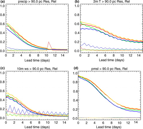
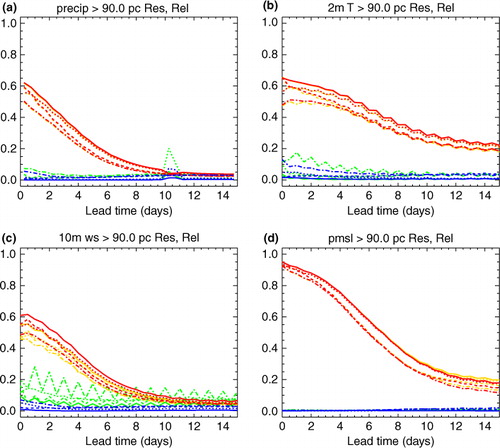
Fig. 2 The resolution (solid) and reliability (dotted) components of the Brier Skill Score (BSS) for the 90th percentile of the local ‘alternate month’ climatology as described in the text. Results are shown for the perturbed members of the raw ECMWF (red), Met Office (green) and NCEP (blue) ensemble systems, and the simple aggregation of all these members (orange). The variables are: (a) 12 h-accumulated precipitation, (b) two-metre temperature, (c) 10-metre wind speed and (d) pressure at mean sea level.

In this paper, the Brier Skill Score (BSS) is used as the main tool for measuring overall forecast performance. This considers the full PDF predicted by the ensemble (as opposed to, say, just the mean and spread), and allows performance for different types of event to be distinguished through the choice of threshold. Related tools such as the reliability and Relative Operating Characteristics (ROC) diagrams can be used to help understand the results. Details of all these verification techniques can be found in Wilks (2006). The overall BSS measures the proximity of the forecast probabilities to the ideal of 1.0 when the event occurs and 0.0 when it does not. This perfect forecast scores a BSS of 1.0, whilst a system no better than always forecasting a probability equal to the climatological frequency of the event scores 0.0. The plots show the BSS split into the two components mentioned in the Introduction. The ‘resolution’ (solid lines in Fig. 2) measures the fundamental ability to forecast different probabilities for situations where the event is more or less likely, regardless of their numerical value. The reliability penalty (dotted lines in Fig. 2) measures the weighted mean square difference between the forecast probabilities and the frequency with which the event occurs in each case. This decomposition is useful for probing the action of a calibration scheme, particularly one which aims to eliminate unreliability without harming statistical resolution. The overall BSS is the resolution minus the reliability penalty.

One could choose a set of fixed thresholds appropriate to each variable and find the BSS for each of these. However, this has a number of disadvantages. Since the thresholds are chosen separately for each variable, they do not provide a direct comparison of performance for ‘equivalent’ thresholds of different variables. Many fixed thresholds will only be ‘in doubt’ for particular locations or seasons, with the threshold outside the range of climatology in all other cases. This has two consequences. First, the model receives credit for knowing the spatial or seasonal variation in climatology (‘false skill’; Hamill and Juras, 2006). Second, the score is actually determined by performance for a few locations at particular times of year, resulting in a high level of noise.

To mitigate these problems, this paper presents results for thresholds which are chosen indirectly, via quantiles of a climatology which varies in both space and time. The forecast now has to beat this climatology to receive a positive skill score. The resulting lower scores help to emphasise the differences between systems. The approach tends to increase the magnitude of the reliability penalty compared to fixed thresholds, which is helpful when evaluating a scheme designed to eliminate unreliability. Since a given quantile should be equally likely to be exceeded at any location or time of year, the final score makes equal use of all locations and seasons, which should improve the signal-to-noise ratio. A separate climatology is also used for each time of day (00 and 12 UTC). Since the thresholds are effectively parameterised in terms of their local rarity, one can meaningfully compare system performance for the same quantile of different variables. One additional advantage for this particular study is that the continuously varying values of the climatological thresholds will explore all possible relationships with the fixed thresholds used for training the reliability calibration scheme.

Ideally, one would choose the thresholds based on a long-term climatology. However, this would require further data to be obtained which matched the spatial and temporal characteristics of the main observations. There is no long-term archive of EuroPP data, and in any case that system has not been designed for long-term stability. There is also little point evaluating performance for thresholds which are not reasonably well-sampled within the 2-yr verification period. Instead, a simple approach is used whereby the verification thresholds for a given month are taken from the 5×5-gridpoint region centred on the gridpoint of interest for the same month in the other year of the overall 2-yr period. By contrast, Flowerdew (2012) took the thresholds from the same month in the same year as the verification. This had the advantage that each quantile is exceeded exactly the specified number of times for each location and month. However, it gives the climatology an unfair advantage as a reference forecast, since it knows more precisely than an independent climatology exactly where the events will occur within the month. This leads to some very large and unreasonable reliability penalties for the outer quantiles of some variables. It is not clear whether or not the in-sample climatology actually gives an incorrect order of preference to the different forecasting systems, but in any case the independence of the ‘alternate month’ approach simplifies the interpretation of the reliability penalty.

Since the ‘alternate month’ thresholds are drawn from 25 nearby gridpoints over a single month, they do not provide a particularly good estimate of the long-term climatology. However, this is not essential: all that is needed is a prediction independent of the verification period that takes out much of the spatial and seasonal variation. The optimal degree of averaging can be estimated as that which minimises the apparent skill of the forecasts: averaging over too large an area increases apparent skill because it smoothes out some of the detectable climatological variations, whilst averaging over too small an area increases apparent skill because noise starts to dominate signal in the estimated climatology. The above configuration was chosen as that which approximately minimises the apparent skill scores for two-metre temperature at moderate quantiles. Since the climatology involves some noise, a good climatological forecast can still beat it, and so some false skill remains, e.g. in resolution scores not asymptoting to zero. There is also a tendency to underestimate outer quantiles by the following mechanism. In most cases, a given month will contain more extreme events in one year than the other. The thresholds derived from the less extreme year will let through a large number of events from the more extreme year, overpopulating the outer quantiles. The performance for more extreme events is considered in section 4.4 using thresholds drawn from the climatology of the whole ‘alternate year’, sacrificing seasonal variation in order to get the observed event frequency closer to the requested nominal quantile.

In the interests of brevity, Fig. 2 and most later plots only show results for a single quantile. Results for other quantiles are generally similar, with a gradual decline in skill towards more extreme quantiles in most cases (see also section 4.4 below). As expected, overall skill tends to decline with lead time. This is driven by the fundamental ability to distinguish events from non-events (resolution), whereas reliability often improves with lead time as the ensemble expands towards climatology. Results for temperature and wind speed show a marked diurnal cycle, with midnight harder to forecast than midday for high quantiles. Performance for precipitation and sea-level pressure is less dependent on the time of day.

Sea-level pressure is a far better forecast than any of the other variables, with higher initial scores, and the decline not starting to tail off until around T+10 d. Temperature has the next highest initial scores, with a relatively slow decline in skill. The skill for precipitation and wind speed decreases more quickly, particularly for higher quantiles.

The precipitation results for ECMWF (and thus to a lesser extent for the multimodel combination) show a dip in resolution and a spike in reliability penalty for the 12 h period just following the increase in grid spacing at T+10 d. This may be largely caused by the way accumulations across the grid change are handled within the TIGGE archive, rather than indicating a problem with the ECMWF forecast itself. However, it should be noted that the ECMWF performance is also below-trend for the second 12 h period following the transition, which is not subject to these technical issues. As one might expect, some results (such as ROC area for high precipitation amounts and some quantiles of sea-level pressure climatology, not shown) show a permanent drop in performance associated with the increase in grid spacing.

As might be expected from their respective grid spacings, ECMWF generally provides the best single-model forecast, followed by the Met Office and NCEP. Against EuroPP, the Met Office forecasts perform relatively well at short lead times. This may partly reflect a successful short-range focus for this system, but may also be unfairly enhanced by the contribution of related Met Office models to the EuroPP analyses themselves. Verification against Met Office or ECMWF analyses or short-range forecasts (not shown) results in a stronger preference for the corresponding system, as expected. Verification against truly independent observations would be needed to definitively establish the relative value of the different systems, but this is not the focus of the present paper. However, one robust result is worth noting: the multimodel combination is almost never worse than the best single model. Even against ECMWF analyses, it provides some small advantages. The true advantage against independent observations would presumably be larger than this, perhaps closer to the results shown here against EuroPP.

4.2. Reliability calibration

Figure 3 illustrates the performance of the reliability calibration method, for the same variables and quantiles as were shown in Fig. 2. The calibrated resolution/reliability are shown in red/blue respectively, with the corresponding raw results in orange/green for comparison. Since colour is used to highlight the impact of calibration, the different forecast sources are now denoted by linestyles as indicated in the caption.

Fig. 3 The resolution (orange/red) and reliability (green/blue) components of the BSS for the same events as Fig. 2, but showing results before (orange/green) and after (red/blue) application of the reliability calibration scheme. Results are shown for the ECMWF (dotted), Met Office (dashed) and NCEP (dot–dashed) ensemble systems, and the simple aggregation of all these members (solid). Panels (a)–(c) use the standard configuration. The calibration for panel (d) aggregates the training data with fixed 20-point spatial padding and re-projects onto four replicas of the original ensemble, with verification using 186 probability bins, as discussed in the text.

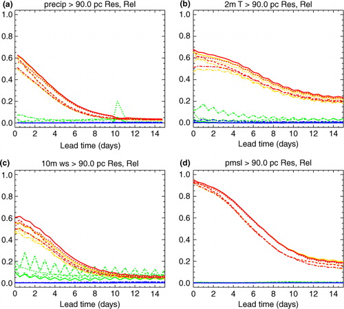
The calibration is generally very effective at its main objective of eliminating unreliability. The overall benefit in terms of skill thus depends on how reliable the raw forecasts were: the poorer systems will tend to improve more than the better systems. However, the better systems are generally still improved, or at least not harmed, and the calibrated multimodel ensemble generally remains superior to the best calibrated single-model results. Some improvements in statistical resolution are also evident. This might seem surprising, since an overall relabeling of probability values cannot change the resolution component of the BSS. When the precipitation results are regenerated using a calibration which is forced to always average the training over the whole domain, much of the resolution benefit is indeed removed (not shown). This suggests that the original resolution improvement results from the spatial variations in the mapping from raw to calibrated probabilities, which is improving the ability to distinguish cases in which the threshold is more or less likely to be exceeded. In other words, an improvement in local reliability is measured as an improvement in overall resolution.

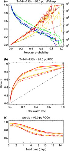
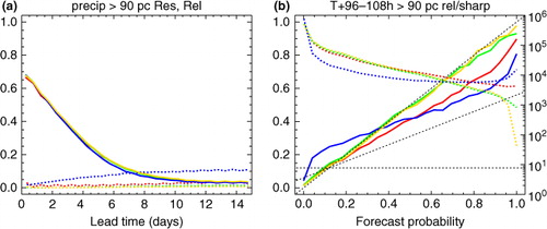
The one detrimental impact observed for the 1–99th nominal percentiles of variables other than sea-level pressure is some losses of the area under the ROC curve (and, to a lesser extent, BSS resolution) at long lead times for the outermost quantiles. ROC curves show the hit and false alarm rates which would be achieved by acting at each available probability threshold, providing an alternative measure of statistical resolution (Wilks, 2006). The problem is illustrated in Fig. 4 for the 99th percentile of precipitation, which shows a slight loss in ROC area for the NCEP and Met Office ensembles around T+4–9 d (bottom panel). As usual, the calibration is quite effective at diagonalising the corresponding reliability diagrams (top panel), bearing in mind the noise in the verification. However, this requires reducing the forecast probabilities for this rare event (green/blue lines). This reduces the number of ensemble members above the threshold, eliminating some cases in which just one member exceeded the threshold. This reduces the hit rate at the rightmost kink of the ROC curve (middle panel), and one can imagine a similar effect applying to the BSS resolution (less dramatically due to the weighting by frequency of occurrence which is built into the BSS). Thus, it seems that small losses of resolution such as these are an inevitable consequence of the twin requirements of statistical reliability and re-projection onto a finite number of equally weighted ensemble members. One simple remedy, employed in a few cases below, is to re-project the calibrated CDF onto not one but several replicas of the original raw ensemble. This provides more members which can thus represent more quantiles of the calibrated CDF, including extra detail in the tails. For the larger ensembles, the verification must use a correspondingly large number of probability bins to see the full benefit of this approach (this has negligible impact other than adding noise when verifying raw forecasts, compared to the 50 bins used for all other results). Replicating the raw ensemble is not a perfect solution, since the repeated patterns will introduce small spurious long-range correlations into the implied covariances. More independent extra members might be obtained by forming a ‘lagged’ ensemble including earlier cycles of each forecast system.

Fig. 4 The impact of reliability calibration on the 99th percentile of precipitation. Calibrated results are shown in red/blue, with the corresponding raw results in orange/green. Linestyles represent the different underlying forecast systems as in Fig. 3. The panels show: (a) reliability (orange/red) and forecast frequency (also known as sharpness, green/blue, using the logarithmic scale to the right of the plot) as a function of the forecast probability and (b) the relative operating characteristics (ROC) curve, both covering the 12 h accumulation period starting at T+6 d, and (c) the area under the ROC curve, as a function of lead time. Black dotted straight lines show the ideal, ‘no skill’ and ‘no resolution’ conditions.

The results for sea-level pressure (Fig. 3d) are less positive than for other variables. This variable is inherently large scale, so that there are fewer systematic errors arising from the limited spatial resolution of the medium-range models. This is reflected in the high statistical resolution and low reliability penalty of the raw forecasts, leaving little prospect for improvement by calibration. The reliability calibration is effective at removing what unreliability there is. It also slightly improves the resolution at short lead times. Two further steps have been taken to reduce the slight detriments at longer lead times. Firstly, the calibration has been forced to use 20° of spatial padding throughout, rather than the standard dynamic aggregation process. It seems that the 200 samples requirement which works well for other variables is not sufficient for the coherent features found in sea-level pressure, and that more averaging is needed to keep the signal-to-noise ratio sufficiently high. Secondly, the calibrated probabilities have been re-projected onto four replicas of the original ensembles, with 186 probability bins (twice the number of members in the multimodel combination) being used in the verification. This brings a small improvement to NCEP resolution, and a larger improvement to ROC area at higher quantiles (not shown). However, despite these improvements, the calibration remains slightly detrimental to the resolution of the better systems at long lead times. It may simply not be worth attempting to calibrate this variable. One of the attractive features of both calibration methods presented here is that they preserve relationships not only within the calibrated ensemble but also between the calibrated and raw ensembles. Thus, one can restrict calibration to just those variables for which it is beneficial, whilst maintaining coherence with the uncalibrated variables. Indeed, one could apply different calibration methods to different variables, provided they all preserve spatial structure through the member identity.

4.3. Climatology calibration

In this section, the reliability calibration results are compared to the climatology calibration introduced in section 2.1. Figure 5 shows the impact of climatology calibration in the same format as Fig. 3, with the raw results in orange/green. As explained in section 2.1, this method uses a pre-specified degree of spatial padding whose optimal value will be a compromise between the signal-to-noise ratio and the locality of the calibration. Flowerdew (2012) used two-point padding (giving 5×5-gridpoint local regions) for calibrating precipitation. When applied to two-metre temperature, this was beneficial for low and moderate quantiles at short lead times, but generally inferior to the raw forecasts for high quantiles and longer lead times (not shown). Experiments with 3, 5, 10, 20-point and whole-domain padding suggested that 20-point padding is approximately optimal for this variable, producing results that are generally not inferior to the raw forecasts, although not quite as effective as two-point padding for low and moderate quantiles at short lead times. Twenty-point padding was also better for sea-level pressure and the 50th percentile of precipitation, but two-point padding was superior for wind speed and the higher quantiles of precipitation. In each case, Fig. 5 shows the results from the most beneficial configuration tested.

Fig. 5 As Fig. 3, but showing the impact of the climatology calibration scheme. As discussed in the text, training data are aggregated with two-point spatial padding for panels (a) and (c), but 20-point padding for panels (b) and (d).

With these optimisations, the climatology calibration is slightly beneficial to reliability and resolution for precipitation and temperature, with a larger benefit for wind speed. However, the reliability penalty is not eliminated as effectively as direct reliability calibration (Fig. 3), and the resolution improvement is often smaller. For sea-level pressure, climatology calibration is detrimental at long lead times, and again worse than reliability calibration. In fact, reliability calibration is almost uniformly superior or equal to climatology calibration across the 1–99 percentile range tested. This supports the contention that reliability calibration is solving a more general problem than climatology calibration, improving the prediction of case-specific uncertainty in addition to generalised bias.

The climatology calibration is most effective for wind speed, where it significantly reduces the abnormally large reliability penalty of the raw forecasts, as well as improving statistical resolution. To probe the mechanism behind this improvement, Fig. 6 shows the evolution with lead time of the 95th percentile of the climatologies of EuroPP and the three single-model systems. Like the climatology calibration, this diagnostic finds the 95th percentile in each 3-month block for the 5×5 region centred on each gridpoint, excluding data outside the observation domain. It then takes the mean over the eight 3-month blocks, producing a single result for each gridpoint. The plot shows the 10th, 50th and 90th percentiles of this spatial field.

Fig. 6 The 10th (lower dotted lines), 50th (solid lines) and 90th (upper dotted lines) percentiles over space of the mean over 3-month blocks of the 95th percentile of 5×5-gridpoint climatologies for wind speed, presented as a function of lead time for the ECMWF (red), Met Office (green) and NCEP (blue) ensemble systems, and EuroPP (orange). Results are shown for: (a) the raw forecasts, (b) forecasts after climatology calibration, and (c) after reliability calibration.

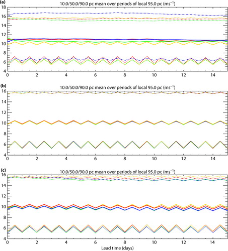
Figure 6a shows that the raw forecasts are generally biased high with respect to EuroPP, although this is not always true for the most windy gridpoints (top lines). The forecasts also disagree amongst themselves as to the climatology, and their relative positions vary as a function of quantile (not shown). These features are not just an artefact of looking at wind speed – they also apply to the gridbox averages of zonal or meridional wind.

The climatology calibration is very effective at homogenising the spatial average forecast climatologies about the observations, as illustrated in Fig. 6b. Correcting these deficiencies is presumably responsible for the relatively large improvement in probabilistic performance shown in Fig. 5c. The reliability calibration targets climatology less directly, as the sum of individually reliable forecast PDFs. It is nonetheless very effective at homogenising moderate quantiles about the observations (not shown). Fig. 6c shows an intermediate example. The calibrated forecasts behave more like the EuroPP climatology, with similar diurnal cycles, but there is some drift with lead time which is more pronounced for outer quantiles and smaller ensembles (Met Office and NCEP). As forecasts become more uncertain with lead time, the ensemble has to expand towards the overall climatology. Accurately representing this with reliable equally likely members placed at fixed quantiles of the calibrated CDF requires a large ensemble, such as a multimodel combination. In principle, more correct climatology might be obtained by distributing each member randomly within its assigned quantile range. However, such noise might harm more important skill measures and spatial relationships. Combining rather than discarding bins that have too few samples may also help to improve the calibrated climatologies. Nonetheless, even the smaller ensembles achieved very low reliability penalties with reliability calibration in Fig. 3c.

4.4. More extreme thresholds

Forecasting extreme weather events is a key responsibility of operational centres such as the Met Office. Ensembles are particularly suited to this task, since these events tend to be inherently unlikely. However, their rarity also increases the difficulty of obtaining sufficient data to calibrate and verify forecasts of such events.

Figure 7 illustrates the performance of the reliability calibration scheme for some rare events. Following the discussion in section 4.1, these plots take the threshold at each gridpoint from the 0.1 or 99.9th percentile of the local 5×5 region for the whole ‘alternate year’ of the 2-yr verification period. Although the observed frequencies (just over 0.3% for temperature and 0.1% for precipitation and wind speed) do not quite reach the nominal quantile values, they still correspond to the outermost one or two events per gridpoint in the 2-yr period. On the other hand, the availability of one or two events at each of the 1532 verification gridpoints helps to keep some control over the verification noise. Nonetheless, the verification for such rare events must be regarded as less certain than the results shown above for more frequent events.

Fig. 7 As Fig. 3, but considering more extreme thresholds taken from the local ‘alternate year’ climatology as described in the text. Panels show the 99.9th percentile of: (a) precipitation, (b) temperature and (c) wind speed, and (d) the 0.1th percentile of temperature. As discussed in the text, the precipitation calibration is allowed to use training data from the whole domain, whilst the temperature calibration is re-projected onto four replicas of the original ensemble, with verification using 186 probability bins.

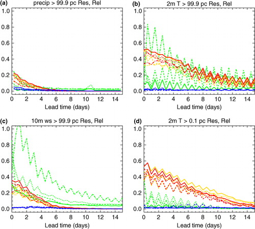
Figure 7 includes some modifications which were found to slightly improve the performance of the reliability calibration. The precipitation calibration has been allowed to gather training data from the whole domain (rather than the usual 20° limit), which slightly improves the BSS for the most extreme quantiles. As in section 4.2, the temperature forecasts have been re-projected onto four replicas of the original ensemble, and verified with 186 probability bins. This gives a slight improvement in BSS resolution, and larger improvements in ROC area, particularly for the smaller ensembles. The extra verification bins lead to a slight increase in the apparent reliability penalty for these rare events, but this is presumably just verification noise, both from the appearance of the reliability diagrams and the fact that the underlying calibrated probabilities are the same in both cases.

Figure 7 shows that some of the raw forecasts have very large reliability penalties, and the calibration is again very effective at almost eliminating these. Statistical resolution is also generally improved, particularly for high temperatures and wind speed. However, there is some loss of resolution for low temperature extremes, where there is also little reliability penalty to correct beyond the shortest lead times.

4.5. Spatial averages

One of the aims of the calibration schemes considered in this paper is to produce ensemble members that retain appropriate spatial, temporal and inter-variable structure. This should extend the benefits of calibration to derived quantities such as regional averages or the output of hydrological models which integrate rainfall in space and time. Whereas authors such as Berrocal et al. (2008) aim to model correlations statistically, the schemes considered in this paper rely on the raw ensemble. No attempt is made to calibrate towards observed correlations, but equally the raw ensemble could provide useful case-specific correlations.

A simple test of this feature can be performed by calibrating at the grid scale but verifying averages over a larger scale (here the 3×3 region centred on each gridbox). The error variance of this average, for example, is the average of the 9×9 matrix representing the error covariance between the individual gridpoints, incorporating both their error variances and the correlations between them. A similar verification technique is used by Berrocal et al. (2008).

The results are shown in Fig. 8a. To simplify the comparison, only results for the Met Office ensemble are shown; results for other systems are similar. The thresholds are derived from an ‘alternate month’ climatology as in section 4.1, except that the input samples are now the 3×3 averages centred on each gridpoint. Raw performance at 3×3 scale (red) is uniformly better than for the original 1° grid (Fig. 2a), perhaps because it gets closer to the effective resolution of the underlying models. Direct calibration at 3×3 scale (orange) produces a similar positive impact to calibration at 1° scale (Fig. 3a).

Fig. 8 The performance of forecasts derived from the Met Office ensemble for the 90th percentile of the 3×3 average of precipitation centred on each gridpoint. The panels show: (a) resolution (solid) and reliability (dotted) components of the BSS as a function of lead time, and (b) reliability (solid) and forecast frequency (dotted) for the 12 h accumulation period starting at T+4 d. Results are shown for the raw forecasts (red), direct reliability calibration of the 3×3 averages (orange), and the 3×3 averages implied by reliability calibration of 1° data with the standard member assignment following the raw ensemble (green) and random member assignment (blue).

The key question is whether the ensemble reconstruction method allows calibration at the grid scale to produce good 3×3 averages. These results are shown by the green lines. On the whole, these achieve similar performance to calibration at 3×3 scale, improving on the raw forecasts. In particular, the reliability penalty is reduced by almost the same extent as direct calibration at 3×3 scale. Indirect calibration does produce poorer BSS resolution and ROC area scores than direct calibration for the smaller ensembles at longer lead times. However, this effect is weak or absent for the larger ensembles (not shown), and indeed the indirect approach sometimes produces superior resolution at short lead times.

The blue lines show the performance of indirect reliability calibration when the members are assigned randomly to quantiles, rather than following the raw ensemble. This amounts to neglecting the spatial relationships embodied within the raw ensemble. It does not change the grid-scale probabilities, but at 3×3 scale it performs much worse than even the raw forecasts, particularly for the reliability of lower quantiles.

Figure 8b shows one of the reliability diagrams which contribute to Fig. 8a. This clearly illustrates the positive impact of both direct and indirect reliability calibration in drawing the raw forecasts towards the ideal diagonal. Random quantile assignment, whilst reliable at 1° scale, produces a sub-unit slope for the 3×3 average. This is consistent with the underspread which would be expected from neglecting the covariance terms in the 3×3 variance, which would in turn harm both reliability and resolution.

4.6. Derived variables

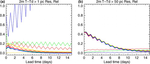
In addition to spatial and temporal structure, the ensemble reconstruction step employed by the reliability calibration scheme should preserve the relationships between variables. This property is briefly tested in this section using the physically motivated example of dewpoint depression (temperature minus dewpoint temperature). Whereas dewpoint temperature essentially measures specific humidity, dewpoint depression is more like relative humidity.

The results are shown in Fig. 9. The test uses the same four configurations as the previous section, and again only the Met Office ensemble is shown (the impact on other forecast sources is qualitatively similar). The raw forecasts for dewpoint depression (red) are much poorer than either of the input variables (e.g. Fig. 2b). Direct reliability calibration (orange) is effective at improving the resolution and largely eliminating the reliability penalty, particularly for low quantiles. Indirect calibration (green) via temperature and dewpoint improves on the raw forecasts for most quantiles, but is harmful to the very lowest quantiles (Fig. 9a), and quite a bit less effective than direct calibration. The difficulty with low quantiles may be related to the fact that these involve small differences between the calibrated forecasts of temperature and dewpoint. Random quantile assignment neglecting the inter-variable relationships (blue) is generally poor, leading to reliability penalties that rise with lead time, particularly for the outer quantiles. However, it does seem beneficial for the 50th percentile (Fig. 9b), where it achieves similar reliability to direct calibration. This may indicate that the raw ensemble correlations are too strong for this portion of the dewpoint depression climatology.

Fig. 9 The resolution (solid) and reliability (dotted) components of the BSS from the Met Office ensemble for the: (a) 1st and (b) 50th percentiles of two-metre dewpoint depression. Results are shown for the raw forecasts (red), direct reliability calibration of dewpoint depression (orange), and the dewpoint depression implied by reliability calibration of temperature and dewpoint temperature with the standard member assignment following the raw ensemble (green) and random member assignment (blue).

5. Discussion

Although ensemble forecasting systems are based on physical laws and the Monte Carlo principle, their finite grid spacing and other approximations lead to systematic errors in climatology and forecast probabilities which can be improved by statistical post-processing. This paper has presented a novel calibration framework, which directly targets statistical reliability whilst making minimal assumptions about the underlying distributions. Instead, it tries to make the greatest possible use of the original physically-based forecasts, including their spatial, temporal and inter-variable structure.

The calibration method has been applied to three leading medium-range ensemble forecasting systems, and their combination into a multimodel ensemble. The evaluation considered a range of surface variables over a European domain for a 2-yr period. Although explicit confidence intervals have not been calculated, the consistency of results as a function of lead time, threshold, variable, verification score and in particular across the different underlying forecasting systems suggests the conclusions are trustworthy. Particular attention has been paid to the BSS evaluated against climatological thresholds, and its decomposition into reliability and resolution components. The calibration largely eliminates the reliability penalty whilst generally preserving or enhancing statistical resolution. In most cases, this improvement seems to extend even to more extreme thresholds. The multimodel combination, being quite reliable to start with, is improved less, but remains almost uniformly competitive with or superior to the best single-model ensemble.

The reliability calibration was compared with a Local Quantile-Quantile Transform, an established calibration method which generalises bias correction. This ‘climatology calibration’ is generally very effective at homogenising the average forecast climatologies about the observations. Reliability calibration indirectly achieves similar results for moderate quantiles, but seems to require a large ensemble to limit drifts in the outer quantiles of some variables. Nevertheless, the probabilities remain statistically reliable throughout and the overall BSS are superior to climatology calibration.

Two main deficiencies were identified in the univariate aspects of the reliability calibration. The requirement to re-project onto a finite set of ensemble members can lead to some losses of ROC area, and to a lesser extent BSS resolution. This problem can be alleviated using several replicas of the original ensemble for the re-projection step. However, some loss of resolution remains for low temperature extremes. Sea-level pressure is also very challenging to calibrate, primarily because the raw forecasts are so good. A lot of averaging seems to be required to ensure the adjustment adds signal rather than noise. In practice, it may be better simply not to calibrate such variables.

A test based on spatial averages of precipitation suggests the ensemble reconstruction approach is effective at preserving useful spatial structure from the raw ensemble. A similar test deriving dewpoint depression from temperature and dewpoint showed more modest performance, generally improving on the raw forecasts, but not as much as direct calibration. Where products or downstream systems such as hydrological models require particular combinations of variables, it may be better to calibrate these directly rather than rely on inter-variable relationships. This should not be too great a burden, assuming the set of relevant variables is discrete and fairly small. It is much more important that the calibration preserves useful spatial and temporal structure, since deficiencies in these aspects cannot be so readily overcome by direct calibration.

Section 2.2 outlined various ways in which the reliability calibration method might be improved, including the details of spatial aggregation, the treatment of extremes, and the interpolation/extrapolation of reliability diagrams between/beyond the training thresholds. The key to obtaining reliable results is that every calibrated probability is interpolated from relevant observed event frequencies. In the initial implementation presented here, the predictor was the raw probability to exceed the same threshold, but this is not essential. One could, for example, add additional predictors such as the ensemble mean or the forecast probability for another threshold. This might help to improve resolution scores by indicating proximity to the target threshold, particularly for ensembles which are underspread. However, a balance would need to be struck with the statistical noise implied by more finely divided training data. Where the raw forecasts suffer from significant bias, statistical resolution might also be improved by preceding the reliability calibration with a climatology calibration, so that the intermediate members cross the observational threshold when the raw forecasts cross its model-world equivalent. This approach could be particularly beneficial for the multimodel combination, since it provides a way to correct model-specific biases in addition to the overall mean bias.

In the Met Office, the reliability calibration framework is being considered as a potential basis for future operational post-processing of gridded ensemble data. This holds the promise of a calibrated yet spatially and temporally consistent basis for mapped products, site-specific calibration and downstream systems such as hydrological models. In the future, we hope to benchmark the reliability calibration scheme against a wider variety of methods, and develop real-time demonstration products suitable for evaluation by operational forecasters.

6. Acknowledgements

The author thanks Stephen Moseley for information on the EuroPP dataset, and Neill Bowler and Richard Swinbank for useful discussions during the development of this work. Anonymous reviewers provided many constructive comments which helped to improve the clarity of the manuscript. The results presented in this paper were prepared using funding from the European Union FP7 project GEOWOW (grant agreement 282915).

References

- Applequist S. , Gahrs G. E. , Pfeffer R. L . Comparison of methodologies for probabilistic quantitative precipitation forecasting. Weather Forecast. 2002; 17: 783–799.
- Atger F . Verification of intense precipitation forecasts from single models and ensemble prediction systems. Nonlinear Processes Geophys. 2001; 8: 401–417.
- Berrocal V. J. , Raftery A. E. , Gneiting T . Probabilistic quantitative precipitation field forecasting using a two-stage spatial model. Ann. Appl. Stats. 2008; 2: 1170–1193.
- Bougeault P. , Toth Z. , Bishop C. , Brown B. , Burridge D. , co-authors . The THORPEX grand global ensemble (TIGGE). Bull. Am. Meteorol. Soc. 2010; 91: 1059–1072.
- Bremnes J. B . Improved calibration of precipitation forecasts using ensemble techniques. Part 2: Statistical calibration methods. 2007. met.no report 04/02007. Norwegian Meteorological Institute, Oslo, Norway.
- Coelho C. A. S. , Stephenson D. B. , Doblas-Reyes F. J. , Balmaseda M. , Guetter A. , co-authors . A Bayesian approach for multi-model downscaling: seasonal forecasting of regional rainfall and river flows in South America. Meteorol. Appl. 2006; 13: 73–82.
- Ferro C. A. T . A probability model for verifying deterministic forecasts of extreme events. Weather Forecast. 2007; 22: 1089–1100.
- Flowerdew J . Calibration and Combination of Medium-Range Ensemble Precipitation Forecasts. 2012. Forecasting Research Technical Report 567. Met Office, Exeter, UK.
- Flowerdew J. , Bowler N. E . Improving the use of observations to calibrate ensemble spread. Q. J. Roy. Meteorol. Soc. 2011; 137: 467–482.
- Fraley C. , Raftery A. E. , Gneiting T . Calibrating multimodel forecast ensembles with exchangeable and missing members using Bayesian Model Averaging. Mon. Weather Rev. 2010; 138: 190–202.
- Gneiting T. , Raftery A. E. , Westveld III A. H. , Goldman T . Calibrated probabilistic forecasting using ensemble model output statistics and minimum CRPS estimation. Mon. Weather Rev. 2005; 133: 1098–1118.
- Golding B. W . Nimrod: a system for generating automated very short range forecasts. Meteorol Appl. 1998; 5: 1–16.
- Hagedorn R. , Buizza R. , Hamill T.M. , Leutbecher M. , Palmer T. N . Comparing TIGGE multimodel forecasts with reforecast-calibrated ECMWF ensemble forecasts. Q. J. Roy. Meteorol. Soc. 2012; 138: 1814–1827.
- Hagedorn R. , Hamill T. M. , Whitaker J. S . Probabilistic forecast calibration using ECMWF and GFS ensemble reforecasts. Part I: two-metre temperatures. Mon. Weather Rev. 2008; 136: 2608–2619.
- Hamill T. M . Verification of TIGGE multimodel and ECMWF reforecast-calibrated probabilistic precipitation forecasts over the contiguous United States. Mon. Weather Rev. 2012; 140: 2232–2252.
- Hamill T. M. , Colucci S. J . Verification of Eta-RSM short-range ensemble forecasts. Mon. Weather Rev. 1997; 125: 1312–1327.
- Hamill T. M. , Hagedorn R. , Whitaker J. S . Probabilistic forecast calibration using ECMWF and GFS ensemble reforecasts. Part II: precipitation. Mon. Weather Rev. 2008; 136: 2620–2632.
- Hamill T. M. , Juras J . Measuring forecast skill: is it real or is it the varying climatology?. Q. J. Roy. Meteorol. Soc. 2006; 132: 2905–2923.
- Hamill T. M. , Whitaker J. S . Probabilistic quantitative precipitation forecasts based on reforecast analogs: theory and application. Mon. Weather Rev. 2006; 134: 3209–3229.
- Harrison D. L. , Driscoll S. J. , Kitchen M . Improving precipitation estimates from weather radar using quality control and correction techniques. Meteorol. Appl. 2000; 6: 135–144.
- Johnson C. , Swinbank R . Medium-range multimodel ensemble combination and calibration. Q. J. Roy. Meteorol. Soc. 2009; 135: 777–794.
- Liu Z. Q. , Rabier F . The interaction between model resolution, observation resolution and observation density in data assimilation: a one-dimensional study. Q. J. Roy. Meteorol. Soc. 2002; 128: 1367–1386.
- Park Y.-Y. , Buizza R. , Leutbecher M . TIGGE: preliminary results on comparing and combining ensembles. Q. J. Roy. Meteorol. Soc. 2008; 134: 2029–2050.
- Primo C. , Ferro C. A. T. , Jolliffe I. T. , Stephenson D. B . Calibration of probabilistic forecasts of binary events. Mon. Weather Rev. 2009; 137: 1142–1149.
- Raftery A. E. , Gneiting T. , Balabdaoui F. , Polakowski M . Using Bayesian model averaging to calibrate forecast ensembles. Mon. Weather Rev. 2005; 133: 1155–1174.
- Richardson D. S . Skill and relative economic value of the ECMWF ensemble prediction system. Q. J. R. Meteorol. Soc. 2000; 126: 649–667.
- Saetra Ø. , Hersbach H. , Bidlot J. , Richardson D. S . Effects of observation errors on the statistics for ensemble spread and reliability. Mon. Weather Rev. 2004; 132: 1487–1501.
- Schefzik R. , Thorarinsdottir T. L. , Gneiting T . Uncertainty quantification in complex simulation models using Ensemble Copula Coupling. Stat Sci. 2013; 28: 616–640.
- Stensrud D. J. , Yussouf N . Reliable probabilistic quantitative precipitation forecasts from a short-range ensemble forecasting system. Weather Forecast. 2007; 22: 3–17.
- Wilks D. S . Statistical Methods in the Atmospheric Sciences. 2006; 2nd ed, Elsevier, Amsterdam.
- Wilks D. S . Extending logistic regression to provide full-probability-distribution MOS forecasts. Meteorol. Appl. 2009; 16: 361–368.