Sensitivity of simulated regional Arctic climate to the choice of coupled model domain

Abstract

The climate over the Arctic has undergone changes in recent decades. In order to evaluate the coupled response of the Arctic system to external and internal forcing, our study focuses on the estimation of regional climate variability and its dependence on large-scale atmospheric and regional ocean circulations. A global ocean–sea ice model with regionally high horizontal resolution is coupled to an atmospheric regional model and global terrestrial hydrology model. This way of coupling divides the global ocean model setup into two different domains: one coupled, where the ocean and the atmosphere are interacting, and one uncoupled, where the ocean model is driven by prescribed atmospheric forcing and runs in a so-called stand-alone mode. Therefore, selecting a specific area for the regional atmosphere implies that the ocean–atmosphere system can develop ‘freely’ in that area, whereas for the rest of the global ocean, the circulation is driven by prescribed atmospheric forcing without any feedbacks. Five different coupled setups are chosen for ensemble simulations. The choice of the coupled domains was done to estimate the influences of the Subtropical Atlantic, Eurasian and North Pacific regions on northern North Atlantic and Arctic climate. Our simulations show that the regional coupled ocean–atmosphere model is sensitive to the choice of the modelled area. The different model configurations reproduce differently both the mean climate and its variability. Only two out of five model setups were able to reproduce the Arctic climate as observed under recent climate conditions (ERA-40 Reanalysis). Evidence is found that the main source of uncertainty for Arctic climate variability and its predictability is the North Pacific. The prescription of North Pacific conditions in the regional model leads to significant correlation with observations, even if the whole North Atlantic is within the coupled model domain. However, the inclusion of the North Pacific area into the coupled system drastically changes the Arctic climate variability to a point where the Arctic Oscillation becomes an ‘internal mode’ of variability and correlations of year-to-year variability with observational data vanish. In line with previous studies, our simulations provide evidence that Arctic sea ice export is mainly due to ‘internal variability’ within the Arctic region. We conclude that the choice of model domains should be based on physical knowledge of the atmospheric and oceanic processes and not on ‘geographic’ reasons. This is particularly the case for areas like the Arctic, which has very complex feedbacks between components of the regional climate system.

• regional climate model
• Arctic Ocean
• sea ice
• downscaling
• REMO
• coupled model

1. Introduction

The Arctic climate system has experienced dramatic changes during the past three decades. These changes include a prominent decrease in sea ice coverage (e.g. Screen and Simmonds, 2010; Stroeve et al., 2012) and thinning of the sea ice (Maslanik et al., 2011). Observed also are a temperature increase of the oceanic intermediate water layer (Polyakov et al., 2005; Dmitrenko et al., 2008), unprecedented accumulation of fresh water in the Beaufort Gyre (Proshutinsky et al., 2009; Morison et al., 2012) and the rise of the mean coastal sea level (Proshutinsky et al., 2004; Henry et al., 2012).

Large-scale atmospheric circulation is one of the main driving forces of the Arctic climate, at least on time scales from days to decades. The large-scale atmospheric variability over the mid- and high-latitudes is organised in so-called teleconnections (e.g. Wallace and Gutzler, 1981), linking different parts of the globe and particularly their ‘centres of action’. The leading pattern of variability over the Northern Hemisphere corresponds to the Arctic Oscillation (AO), also called Northern Annular Mode (NAM; Thompson and Wallace, 1998). This is related to the strength of the Northern Hemisphere polar vortex and thus to the temperature difference between the pole and mid-latitudes. The second leading mode of variability corresponds to the Pacific North American (PNA) pattern, a 3-center mode extending over most of the North Pacific and North America (Wallace and Gutzler, 1981). PNA variability is associated with changes of synoptic activity over the North Pacific and weather and climate conditions over most of the North American Continent (e.g. Archambault et al., 2008). Moreover, it has a downstream influence on the North Atlantic area, which may however vary in magnitude in decadal time scales (e.g. Pinto et al., 2011). Over the North Atlantic and Europe, the dominant mode of variability is the North Atlantic Oscillation (NAO; e.g. Hurrell et al., 2003), which is closely related to the AO. The NAO is a measure of the strength of the pressure gradient over the North Atlantic and thus also of the strength of the westerly winds. The NAO is associated with changes in latitude and intensity of the eddy-driven jet over the North Atlantic (e.g. Luo et al., 2007) and also of synoptic activity, temperature and precipitation fields over Europe (e.g. Hurrell et al., 2003; Pinto and Raible, 2012).

Recent studies have suggested that the last three decades have been characterised by changes in the above-mentioned large-scale atmospheric patterns (e.g. Overland and Wang, 2010), either due to multi-decadal natural variability, climate forcing or a combination of both. For example during the 2000s the Dipole Anomaly, which is defined either by the third principal component pattern based on mean sea level pressure (MSLP) data north of 20°N, or by the second principal component pattern based on data northward of 70°N, has apparently become more pronounced and important to many physical processes, such as sea ice variability (Wu et al., 2006; Overland and Wang, 2010). However, there is evidence that a reduction in Arctic sea ice may lead in turn to a negative NAO response and thus to a southward shift of synoptic activity over the North Atlantic (e.g. Strong and Magnusdottir, 2011). However, such a response is fairly weak under current climate conditions when compared to natural climate variability (Screen et al., 2013), and was found to be sensitive to the basic state of the model (Bader et al., 2011). Thus, the bi-directional influences between large-scale atmospheric patterns, Arctic climate and sea-ice variability must be seen as a coupled problem (Serreze and Barry, 2011).

Possible changes in climate over the Arctic simultaneously affect several components of the climate system, and therefore individual components (e.g. sea ice) should not be analysed independently. Numerical models have proven to be an effective tool for studying Arctic climate, and considering lack of in situ observations in this region, they are sometimes the only possibility to obtain comprehensive insights on the details and mechanisms of climate variability. Given the amount of feedbacks in the system, the best approach is to use coupled ocean–sea ice–atmosphere regional high resolution models (e.g. Koenigk et al., 2011, 2013). They are computationally less expensive to run than global setups, while retaining a high enough resolution to study mesoscale coupled processes in the region of interest.

One of the decisions that have to be made during the model setup process is what region the coupled area will cover. It should be large enough to include all regions that are important for simulation of coupled interactions between components of the system under consideration, but also small enough to reduce computational costs and to receive influence from the large-scale atmospheric circulation modes and teleconnection patterns. For the latter aspect, it may be important to include or exclude some of the key regions, in which generation of variability for a certain area is particularly relevant. Similar questions arise in models that use unstructured triangular meshes: in which regions must one increase the resolution of the mesh, and in what other regions is it reasonable to use lower resolution?

Recently, Mikolajewicz et al. (2005) and Döscher et al. (2010) used an ensemble of initial conditions of regional pan-Arctic coupled models to explore how strongly the Arctic variability is forced by large-scale conditions outside the region and how much of this variability is generated by internal processes and interactions in the Arctic Ocean, atmosphere and sea ice. Using the methodology developed by Mikolajewicz et al. (2005), they were able to separate the relative contributions of inter-annual ‘internal variability’ generated within the model domain, and ‘common variability’ generated outside the model domain. They found that common variability is stronger than internal variability for most of the climate variables in the Arctic during 1980s and 1990s, but internal variability can dominate in some areas. However they do not investigate influence of the coupled domain position, assuming that internal variability would just decrease with the domain size. The nudging technique (von Storch et al., 2000; Castro et al., 2005) could help to isolate the internal variability from the common variability. This technique has been proposed as a way of ensuring that the large-scale atmospheric circulation is not altered too much by the regional model, while allowing the regional scales to be developed exclusively by the regional model. However, it has been shown (Alexandru et al., 2008; Omrani et al., 2012) that the nudging parameters should be carefully chosen in order to avoid excessive control of the large-scale atmospheric variability and decrease of the internal variability.

The area of interest in this study is the Arctic Region including the northern part of the North Atlantic (Fig. 1). We investigate what effect inclusion or exclusion of certain regions has on the Arctic climate simulations and how it affects externally and internally generated variability. In particular we address three main questions:

• What is the influence of regional domain configuration on climate simulations over the Arctic region?

• What are the mechanisms responsible for differences between the coupled model simulations over different domains?

• Is it possible to estimate the contribution of internal modes to Artic climate variability?

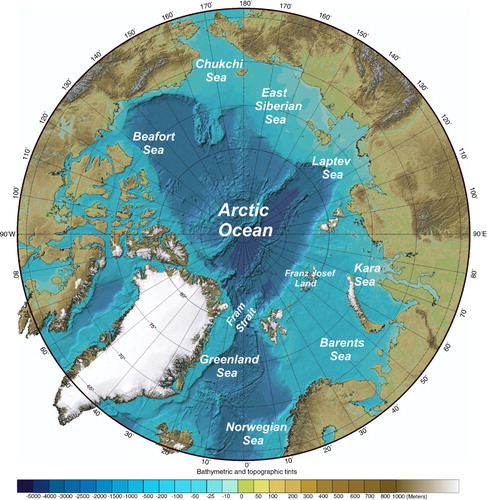
Fig. 1 Arctic Ocean.

The structure of the remaining paper is as follows: Section 2 describes the experimental setup and the datasets. The evaluation of the regional climate for the different setups is presented in Section 3, while the impact on climate variability is discussed in Section 4. A short discussion and conclusion follows.

2. Experimental setup

The REgional atmosphere MOdel (REMO; Jacob and Podzun, 1997; Jacob, 2001) is coupled to the global ocean–sea ice model MPIOM (Marsland et al., 2003) with increased resolution in the Arctic. The models are coupled via the OASIS (which stands for Ocean Atmosphere Sea Ice Soil) coupler (Valcke et al., 2003), which provides the exchange between the ocean and atmosphere models. The OASIS coupler receives sea surface temperature (SST), sea ice thickness (SIT) and concentration data at certain time intervals (the coupling time step) from MPIOM and send them to REMO. Simultaneously, the OASIS coupler receives from REMO heat, water and momentum flux data and transfers them to MPIOM. The simplified coupling procedure is schematically presented in Aldrian et al. (2005), where the authors used the same model components but the sea ice and terrestrial hydrology were not yet included into the coupling. The model validation for the Arctic Ocean is presented in Mikolajewicz et al. (2005).

Exchange between ocean and atmosphere was made using a 6-hour coupling time step. Lateral atmospheric boundary conditions and upper oceanic forcing outside the coupled domain were prescribed using NCEP/NCAR reanalysis (Kalnay et al., 1996) data (the total simulation period was 1948–2007). The global Hydrological Discharge model (HD, Hagemann and Dümenil Gates, 2001), which calculates river runoff, is coupled to both the atmosphere and ocean components. In the coupled model domain, it receives surface runoff and drainage from the atmospheric model and calculates river runoff into the ocean, which is delivered to the ocean model. In the uncoupled model domain, HD reads the same quantities from reanalysis data. The scheme in Fig. 2a illustrates the various interactions between different components of the coupled system.

Fig. 2 MPIOM/REMO/HD Coupling (a) and coupled setups (b). Coloured spherical rectangles on (b): Arctic (violet), Asia (green), Atlantic (red), Pacific (blue), Atlantic–Pacific (black). Domains are defined on REMO grid. Thin black lines – MPIOM grid (every 12th grid line).

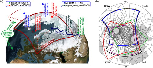
Five different coupled setups (Fig. 2b) were used for five ensemble simulations. The coupled model setups share the same ocean-model configuration. Each ensemble contained five ensemble members. In order to obtain four additional members of the ensemble, a short 4-month run with CO₂ concentration increased by 1 ppm was performed starting from initial conditions of the original run. Data obtained in the runs with increased CO₂ were used as initial conditions for ensemble members, with each of them starting with 1 month lag [i.e. 01 Feb. 1948 (2nd member), …, 01 May 1948 (5th member)]. After this initial perturbation, all the ensemble members were run with exactly the same model parameters and exactly the same boundary conditions.

The coupled domain of each setup includes the Arctic (Fig. 1) and additionally a specific region, that is, Asia, Atlantic, Pacific, in order to investigate the impact of this region on Arctic climate variability (Fig. 2b). The setup with the smallest domain covering the whole Arctic and the northern North Atlantic is called the ‘Arctic’ setup. The others are named according to region of extension. The Atlantic–Pacific (AP) setup was added after we obtained some surprising results from the ‘Pacific’ configuration. This AP setup is an extension of the one to the North Atlantic.

The ocean model has been started from climatological temperature and salinity distributions (Levitus et al., 1998) and run sequentially three times cycling through the period 1948–2000, using forcing data from the NCEP/NCAR reanalysis. Every next time the model was started again from 00:00 01.01.1948 and initialised with the ocean state obtained at the end of the previous cycle, that is, 24:00 31.12.2000. This ‘cyclic’ integration was performed because the ocean model spin-up needs several hundred years, but the longest available consistent reanalysis data set (NCEP/NCAR) is only about 60 yr long. The coupled model simulation for every one of the five setups was started from the end of the third repeat cycle of the uncoupled ocean model (setting the ocean state from 31.12.2000 to 01.01.1948) and from 00:00 01.01.1948 using NCEP/NCAR reanalysis data for the atmosphere.

With the ocean model running uncoupled (i.e. in standalone mode), an inconsistency in fresh water budget arises. On the one hand, precipitation and river runoff are prescribed from reanalysis or observational data. On the other hand, surface evaporation is calculated by the model. To avoid the model drift caused by this inconsistency, a salinity-restoring correction is applied additionally to the natural freshwater fluxes. This correction is implemented by adding to the advection-diffusion salinity equation an additional ‘source’ term of the form −(S−S _obs )/k, where S is the modelled salinity, S _obs is the ‘observed’ salinity to which the computed salinity should be restored, and k is a time constant regulating the restoring speed. The details of the salinity-restoring algorithm implemented in MPIOM are described in Marsland et al. (2003). In our simulations, restoring was performed for the surface layer (0–12 m) towards climatology with a time constant of 180 d. No salinity restoring is applied under sea ice. In the coupled model, inconsistencies in the freshwater budget over the ocean in the uncoupled model domain were also leading to a substantial drift of the model. To overcome this, salinity in the surface layer (0–12 m) was also restored in the first coupled integration towards climatology in the ice-free regions, with the same time constant of 180 d. In subsequent experiments, the restoring was switched off and instead a temporally constant freshwater flux correction calculated for the period 1975–2000 from the first coupled integration was used. We focus on the 1975–2000 period because 1948–1974 was considered to be a transition period from the uncoupled to the coupled state. The advantage of the constant fresh-water flux correction is preservation of the interannual variability. However, the restoring term corrects the sea surface salinity towards climatology, thus strongly reducing the possible drift. As a disadvantage of this approach, we can mention the necessity for additional model runs for obtaining temporally constant freshwater flux corrections. Heat and momentum fluxes are not adjusted.

As a reference for large-scale atmospheric circulation, we consider ERA-40 reanalysis data (Uppala et al., 2005). We preferred using ERA-40 data for comparison, since it represents better the climate variables in the Arctic Ocean (Lindsay et al., 2014) than NCEP/NCAR reanalysis, and it is different from the dataset (i.e. NCEP/NCAR) used to force the model on the boundaries. There is a difference between time spans of model simulations (1948–2007) and the ERA40 reanalysis period (1958–2001). To analyse the modelled climatological means we used the period of 1958–2001 for a consistent comparison with reanalysis data. For the analysis of climate variability in chapter 4, the whole simulation period (1948–2007) was used.

3. Climate – comparison with reanalysis data

In this section, results from different model setups are compared with ERA-40 reanalysis data. With this aim, ensemble means obtained from every five ensemble members for five different model configurations were used. Fig. 3 shows long-term mean 2 m December–January–February (DJF) air temperatures from ERA40, and differences between ensemble means of model simulations and ERA40 (Model – ERA40) for different setups. In general terms, the spatial distribution of temperature differences is quite similar among setups, and differs only in magnitude and on relatively small details. A common feature of all the model configurations is the location of the strongest positive biases over the north-eastern part of the North-American continent, in particular over the Hudson Bay and Canadian Archipelago. Positive biases over Northeast Siberia can also be found for all the setups. Over the Arctic Ocean, the model tends to overestimate the 2 m temperatures over the Kara Sea and Franz Josef Land, and simulates colder than ERA40 temperatures over the Chukchi Sea, except for the Asia and Pacific setups, where biases over the Chukchi Sea are positive. Over the western part of North America and northern parts of Europe, the model shows generally lower temperatures for all the setups. The ‘Pacific’ setup shows largest amplitudes of the temperature biases. The extension of this setup to the North Atlantic (AP) reduces substantially the temperature biases over the Arctic Ocean (Fig. 3f). Differences between NCEP (used here as boundary conditions) and ERA40 are quite small (not shown) and they are largely unrelated to those identified in Fig. 3b–f.

Fig. 3 Mean (1958–2001) ERA40 DJF 2 m temperature and difference Model – ERA40 [K].

Fig. 4 Mean (1958–2001) ERA40 DJF sea level pressure and difference Model – ERA40 [hPa]. Vectors show the anomalous circulation induced in terms of 10 m wind speed (Model – ERA40). Arrow in the right corner – reference vector (5 m/s)

The model domain also has a strong impact on the large-scale atmospheric circulation (Figs. (4–6). The simulated MSLP over the Arctic is particularly important because it affects the sea ice transport and thus the resulting sea ice concentrations and thickness distributions. Therefore, it is one key determinant of the distribution of 2 m temperatures depicted in Fig. 3. The winter MSLP differences between ERA40 and the model setups (Fig. 4) show a more diverse distribution than the 2 m temperatures. Nevertheless, some common features can be identified: for example, there is an overestimation of MSLP over northern parts of Eurasia and the Kara Sea. All the setups also show an underestimation of MSLP over the Far East areas and western North America. The Arctic and Atlantic setups show the smallest biases compared to the reanalysis, while the Pacific and AP setups present an anomalous anticyclonic flow over most of the Arctic. A similar feature has been found by Omrani et al. (2013) in a two-domain ensemble simulation over the European and Mediterranean regions. The authors show that this feature is not of dynamical origin and can be explained by the feedback of the small-scale energetic features on the larger scales. The large positive anomalies seen in Fig. 3e for the Pacific domain are related to the unrealistic atmospheric blocking in the centre of the domain (Fig. 4e). In general terms, and just as for the temperature, the Pacific setup shows the largest differences compared to ERA-40.

Fig. 5 Mean DJF 500 hPa heat transport (v·T) [100 K·m/s] calculated from 6-hourly temperature and wind velocity. Black polygon indicates the common part of all the five setups. Thick arrows schematically represent the Atlantic (red arrows) and Pacific (brown arrows) atmospheric flow.

Fig. 6 Storm track calculated as a standard deviation of bandpass (2.5 – 6 d) filtered DJF 500 hPa geopotential height (m), see main text for more details.

Figure 5 shows an estimation of 500 hPa heat transport for the different model domains. The heat transport is quantified as v·T, with v being the 500 hPa horizontal wind vector (m/s) and T being temperature (K), thus permitting a simple estimation of the heat transport on this pressure level over the Arctic due to the large-scale flow over the area. The large-scale atmospheric circulation of most model configurations shows good agreement with reanalysis data in terms of the flow direction and magnitude. The model simulates heat flow from the North Atlantic to the Russian sector and from the North Pacific to the Canadian sector.

Synoptic activity can be quantified as the standard deviation of the 500 hPa geopotential height fields bandpass-filtered over 2.5–6 d. In this frequency window, the variability associated with low-pressure centres dominates over high-pressure systems, and the resulting variable is commonly denominated storm track (e.g. Blackmon, 1976; Hoskins and Valdes, 1990). The storm track fields for ERA40 and each model domain are shown in Fig. 6. The Arctic, Asia and Atlantic setups show a spatial structure and amplitude that closely resemble those of ERA40, although the storm track extends too far into north-eastern Europe and the North Sea for the Arctic and Asia setups. In the Asia setup, the Atlantic inflow splits into two branches over the Barents and Kara Sea (Fig. 5c, red thick arrow). The northward branch rotates towards the Central Arctic, transporting additional heat from the North Atlantic, leading to a strong warm bias (4–6 K) during winter over that region (Fig. 3c). This might also be related to the storm track anomalies over this area, which display an intensified Siberian storm track (Fig. 6c) compared to ERA, thus enhancing the heat transport towards the Arctic.

However, the storm track intensities are too weak for the AP setup (Fig. 6f). The reduced storm track intensity leads to weaker heat transport over the Arctic, particularly over the North Atlantic and Siberian sectors (Fig. 5f, red arrows). The bias is even larger for the Pacific setup, which shows the strongest bias in winter circulation: the flow is centred too far south over the North Atlantic (Fig. 5e, red arrow), and does not display the rotating northward branch towards the Central Arctic, thus leading to a completely different circulation over the Arctic. The storm track is weaker and more zonal than in ERA40 (Fig. 6e), leading to enhanced heat transport not towards the Arctic but rather towards Asia (Fig. 5e). This bias is related to a MSLP pattern, which shows a strong anticyclonic anomaly (cf. Fig. 4f). As will be discussed in the next section, the choice of model boundary over the North Atlantic destroyed the model consistency in reproducing NAO, leading to a strong dominance of the North Pacific air inflow over the Arctic Ocean. This deficit of the North Atlantic heat transport into the Arctic causes cooling only over the subarctic Eurasian continent, while the Arctic Ocean gets much warmer in winter: up to 4 K in Central Arctic and up to 8 K near the Canadian coast (Fig. 3f).

Winter SIT is presented in Fig. 7. The spatial distribution of SIT in most of the experiments is characterised by accumulation of sea ice in the central part of the Arctic Ocean. This feature is unrealistic, although it has been identified in many coupled ocean–sea ice–atmosphere models (Bitz et al., 2002; Chapman and Walsh, 2007). For a similar model (global coupled ECHAM5/MPI-OM), this feature was found to be mainly related to deficiencies in the model's atmosphere that induce an artificial circulation around the North Pole (Koldunov et al., 2010). The only experiment where the SIT spatial distribution differs is in the Asia setup, where it is to some extent closer to the ‘real world’ distribution. Here, the SIT maximum is shifted towards the Beaufort Gyre and monotonically decreases from the Canadian Archipelago to the East-Siberian Sea. Such distribution is most likely related to the relatively strong and compact cyclonic circulation centred over the northern part of the Canadian Archipelago, which in the Asia experiment turns towards the Beaufort Gyre earlier than in other experiments (Fig. 5c).

Fig. 7 Mean DJF sea ice thickness [m].

Despite differences in the spatial distribution of the atmospheric circulation patterns between experiments, the spatial distributions of SIT remain close to each other (except for the Asia setup), while the mean SIT is considerably different. The latter is consistent with recent results showing that the main driver of the long-term Arctic sea ice variability is the atmospheric thermodynamic forcing (Notz and Marotzke, 2012; Stroeve et al., 2012; Koldunov et al., 2013). The strong reduction of the mean SIT in the Pacific setup reflects the warming caused by the dominant heat transport from the North Pacific (Fig. 7). Extension of the Pacific setup into the North Atlantic (AP setup) leads on average to colder temperatures and drastically changes the ice formation in the coupled domain.

There are also significant differences in the time series of the simulated total sea ice area in recent decades (Fig. 8). The observational sea ice area data for the Arctic Ocean domain were calculated from the ice concentration data from the Nimbus-7 Scanning Multichannel Microwave Radiometer (SMMR) and the Defense Meteorological Satellite Program (DMSP) Special Sensor Microwave/Imager (SSM/I) Passive Microwave Data dataset (Cavalieri et al., 1996) (http://nsidc.org/data/nsidc-0051.html). The Arctic Ocean domain does not include the Nordic Seas, that is, the GIN (Greenland, Irminger and Norwegian) seas, the Barents Sea and the Kara Sea. All configurations show a diminishing trend of the sea ice area, although some differences are evident. For the Arctic and Atlantic setups, the trend is comparatively small, while the Asia and Pacific setups show a more pronounced trend and a lesser extent of the ice-covered area in September. This highlights the impact of the location of the interactive domain on the albedo feedback due to differences in poleward energy transport. Stronger energy transport from the Pacific in summer reduces sea ice extent and concentration, and increases the solar radiation absorbed in the ocean mixed layer in the Chukchi Sea and adjacent regions. This summertime ocean heat gain leads to a thinner ice cap and a stronger ocean heat loss back to the atmosphere. For the AP setup, this mechanism is offset when the domain is extended to the North Atlantic. The colder Atlantic air reduces the summer atmospheric warming and ice melting, preventing the heat gain by the ocean. As a consequence, the ice cap thickens, the heat loss from ocean is reduced and the warm air temperature bias is reduced.

Fig. 8 Sea ice area in Arctic Ocean (x10⁶ km²): March (green), September (red), Annual mean (blue). Thin solid lines – ensemble members, thick solid lines – ensemble means, black dashed lines – observations for corresponding months (Cavalieri et al., 1996).

4. Climate variability

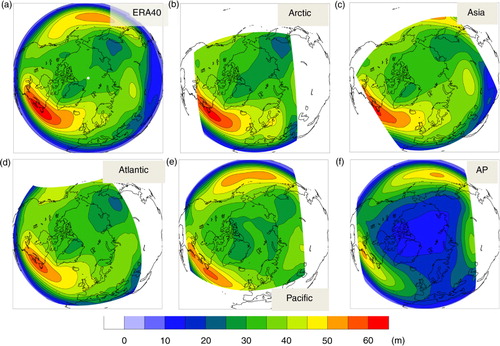
The AO pattern obtained from different model configurations is presented in Fig. 9. The AO was computed as the leading mode of MSLP variability poleward of 20°N (Thompson and Wallace, 1998). Our atmospheric model domains do not cover the whole area required to calculate the AO. To avoid this problem we merged the modelled MSLP and the MSLP of the forcing data set (NCEP). EOF analysis was applied to the combined global reanalysis and regionally modelled MSLP. Because of the merging into the NCEP data set we found it reasonable to compare the resulting AO with those obtained from the NCEP MSLP. In Fig. 9, we show the comparison of the modelled AO with those obtained from NCEP Reanalysis, to analyse possible differences between the modelled data and the data used as boundary conditions.

Fig. 9 Leading EOF of DJF MSLP anomalies over NH (20°–90°N), red spherical rectangles indicates the coupled area.

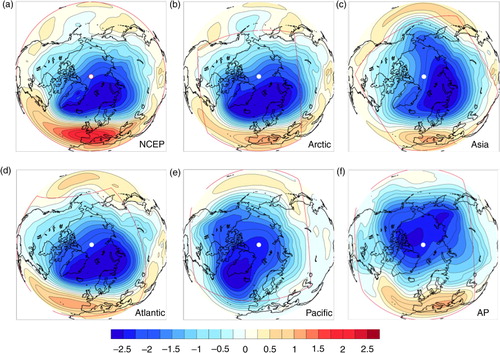
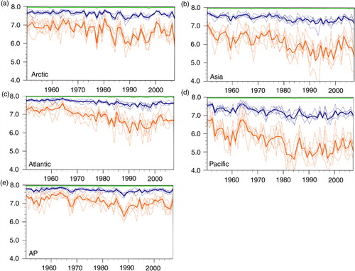
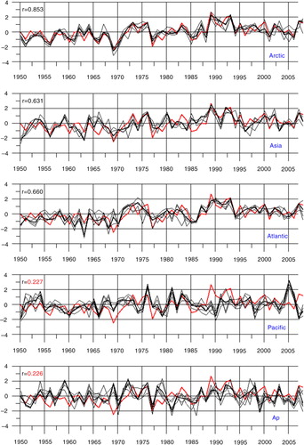
As discussed above, the large-scale atmospheric circulation over the Arctic may be quite different depending on the model domain. In fact, only two out of the five considered setups (Arctic and Atlantic) reproduce the observed AO spatial pattern correctly (Fig. 9). The common feature of these two setups is that the Aleutian Low is prescribed by ‘external forcing’ (i.e. forcing outside the coupled domain). In the other configurations the forcing mostly or totally belongs to the coupled area, and thus can be considered an ‘internal mode’. In these setups (Pacific, Asia, AP), the AO looks quite different compared with the NCEP reanalysis. That is particularly the case for the Pacific setup, where the low pressure area considerably extends southward over the North Atlantic sector. Considering the impact of the different regions on the AO/NAO evolution over time (Fig. 10), we conclude that large-scale modes like the AO are strongly influenced by the atmospheric circulation over the Pacific Ocean. While in the Arctic, Asia and Atlantic setups the simulated AO show a correlation with reanalysis of 0.7–0.8, both of the setups where the coupled area is extended to the Pacific simulate an AO which has a rather low correlation with reanalysis (about 0.2). This fact implies that if one includes the North Pacific into the coupled domain, the AO becomes an ‘internal’ mode, which does not occur when the North Atlantic is included in the coupled area.

Fig. 10 Normalised principal components of the leading EOF of DJF MSLP anomalies (hPa) over NH (20°–90°N) Black thin lines – ensemble members. Black thick line – ensemble mean. Red line – those calculated from NCEP/NCAR MSLP. The numbers on time series plots: correlation between ensemble means and reanalysis, that is, thick black and red line.

In order to estimate the impact of different setups on Arctic climate variability, we now split the model climate variability (following Mikolajewicz et al., 2005) into ‘common’ variability and ‘internal’ variability. The first one should be the ‘common’ part of all the ensemble members, indicating the impact of the lateral forcing that originates from the outer boundaries of the atmospheric model, from the ocean outside the interactive domain and from the top of the atmosphere. Therefore, it can be considered a ‘common’ or ‘external’ variability. It is calculated at each grid point as the standard deviation of the ensemble mean. The internal variability should represent the fluctuations generated within the coupled domain by the model itself and was calculated as the deviation of the ensemble members from the ensemble mean. We estimate the relative importance of external and internal variability by the ‘relative variability index’ (RVI), defined as the logarithm of the common (CV) to internal variability (IV) ratio [log10(CV/IV)]. We prefer the logarithm to the ratio used by Döscher et al. (2010) because it shows better which type of variability is predominant at a given grid point. Positive values indicate that external variability is more important, while negative values indicate that internal variability is prevailing. RVI values in the range −0.1– + 0.1 indicate that the external variability constitutes between 45 and 55% of the total variance. Therefore, we can assume that for these ranges of RVI values both common and internal variability are of similar importance.

The splitting into ‘common’ and ‘internal’ modes and their associated RVI are presented for winter MSLP in Figs. 11 and 2 m temperature in Fig. 12. The corresponding magnitudes for SIT are shown in Fig. 13. Analysing the variability of the large-scale atmospheric circulation from MSLP (Fig. 11) reveals that all model setups generally show a larger common variability than internal variability over the Arctic, especially for the Arctic and Pacific setups, where positive values of RVI cover the whole domain. This is not surprising, because the model MSLP is strongly constrained by the global forcing field. Still, we can see that in all the setups there are regions where internal and common variability are of similar importance, generally located far from the boundaries. The patterns of common variability closely follow the patterns for the corresponding model domain (Fig. 9), e.g. with the Pacific setup showing enhanced variability over the North Atlantic region (unlike other setups). Note that the AP setup shows in general much less variability than the others, both common and internal.

Fig. 11 Mean DJF common (upper row) and internal (centre row) sea level pressure variability. The black polygon indicates the common area of all the five coupled domains. Lower row: log10 of relative variability [common (CV) divided by internal (IV)].

Fig. 12 Mean DJF common (upper row) and internal (centre row) 2 m temperature variability. The black polygon indicates the common area of all the five coupled domains. Lower row: log10 of relative variability [common (CV) divided by internal (IV)].

Fig. 13 Mean DJF sea ice thickness common variability (upper row) and internal variability (centre row). Lower row: log10 of relative variability [common (CV) divided by internal (IV)].

All the configurations have increased internal variability over the Barents and Kara seas despite the differences in model setup. This independence on model setup leads to the conclusion that climate variability in this region strongly depends on the ‘internal’ Arctic. The strongest internal signal is obtained in the Asia setup (Fig. 11g). From all the setups, this one has much more land areas inside the coupled domain. We can speculate that in this case the ocean plays a stabilising role for the coupled ocean–atmosphere–land system, while land has a ‘disturbing’ effect, that is, it generates more internal variability in the atmospheric circulation. This fact has a clear explanation: dynamically, the ocean (being a nearly flat surface) disturbs the atmosphere less than land. Thermodynamically, it has more inertia and damps the temperature variations in the near-surface atmosphere. As a reduced interannual variability is a common feature of global climate models (e.g. Laxon et al., 2003; Koldunov et al., 2010), we can conclude that the coupled region in the AP setup represents a relatively closed system which includes most important areas influencing climate variability in the northern high latitudes. This fact is also reflected by the RVI: its values are between −0.1 and +0.1 over most of the domain.

Figure 12 indicates that the strongest internal signal in the 2 m temperature distribution occurs in the GIN seas and near the Fram Strait. In this region, internal variability is even larger than common variability for almost all the setups, as reflected by the RVI. This can be explained as a consequence of changes in the ice export from the Arctic: variations in exported SIT (Fig. 13) lead to changes in conductive heat flux from the ocean to the atmosphere, and to corresponding changes in the 2 m temperature (Fig. 12). The conductive heat flux from the ocean is inversely proportional to the SIT and proportional to the difference between the ice surface temperature and the freezing temperature (−1.8 C in our setup). This difference can reach more than 30 degrees in winter. The inverse proportionality of conductive heat flux to SIT indicates that sea ice surface temperature depends exponentially on the ice thickness. During winter time, the thick ice (more than 3 m) almost isolates the ocean from the atmosphere. For relatively thin ice (1–2 m) conductive heat flux is the dominant factor providing winter warming of the atmospheric boundary layer in the Arctic. This explains in fact the so-called Arctic amplification (e.g. Screen and Simmonds, 2010) in global warming scenarios: the disappearance of multi-year sea ice in summer due to the greenhouse effect leads to thinner ice cover in winter and stronger conductive heat flux from the ocean, which substantially warms the atmosphere. It is also the reason why the amplification is not so pronounced near Antarctica, as there is almost no multi-year ice in the Southern Ocean.

The variability of the SIT is shown in Fig. 13. In almost all the setups, the common part of the variability looks quite similar. In winter the general drift pattern of Arctic sea ice is determined by the large-scale atmospheric flow. Maxima of common variability can be seen north of Greenland, Canada end eastern Siberia. An exception here is the Pacific setup (Fig. 13d), where a significant part of common variability is located primarily over eastern Siberia. This fact reflects the dominance of atmospheric influence from the North Pacific in this model configuration (Fig. 5e). Both common and internal variability are largest where thick sea ice is piled up by the wind against topography or is driven away from it.

An inspection of the RVI shows that generally the common variability is dominant over the Kara, Beafourt and Chukchi seas and the internal variability is dominant over the Greenland and Barents seas. In the central Arctic, both the internal and common variabilities are of similar importance except for the AP. This is a consequence of the almost closed system character of this setup, as the internal variability is predominant. In the central Arctic, the common variability is typically smaller by a factor 2–3. The internal variability of the DJF ice thickness shows weaker gradients in the Arctic. Whereas in the central Arctic its contribution to the total variance reaches almost 50% (the RVI index is between −0.1– + 0.1), it is close to 20% (RVI index of 0.3–0.4) in the vicinity of coastal areas. Enhanced internal variability extends from the Chukchi Sea to the Central Arctic for the Asia, Atlantic and AP setups (Fig. 13g, h, j). This could indicate enhanced variability in the atmospheric inflow from eastern Siberia into the Central Arctic. The internal variability in the East Greenland Current is higher in all the setups and caused by the large variations in Arctic sea ice export through the Fram Strait.

5. Conclusions and discussion

The coupled response of the Arctic system to different forcings and the relevance of both large-scale atmospheric and regional ocean circulations were analysed with a modelling approach. First, it was evaluated how far the regional domain configuration influences results of climate simulations over the Arctic region. Results show that regional coupled ocean–atmosphere models are sensitive to the choice of modelled area. The different model configurations reproduce differently both the mean climate and its variability. Only two out of five of the used model setups were able to reproduce the Arctic climate as observed under recent climate conditions (ERA-40 Reanalysis), whereas the other three model setups simulate drastically different large-scale atmospheric circulation over the Arctic.

Second, the mechanisms responsible for differences between the coupled model simulations over different domains were analysed. The inclusion or exclusion of selected regions in the model domain allowed us to understand their impact on the Arctic climate variability and predictability. It was found that in the setups where the atmospheric conditions in the North Pacific (in particular the Aleutian low) were prescribed the modelled AO index correlates well with reanalysis (Fig. 10), even if most of the North Atlantic is included in the modelled area. However, the inclusion of the North Pacific makes the Arctic climate much less predictable, to a point that correlations of year-to-year variability with observational data vanish (Fig. 10). This strongly suggests that the North Pacific is a key region influencing the Arctic climate predictability.

Finally, the contribution of internal modes to Artic climate variability was investigated. Ensemble simulations carried out for each model setup enabled the estimation of the relative importance of regional processes (internal variability) and large-scale conditions (common variability) in the Arctic climate system. The amount of internally generated variability is different among the setups and depends on the climate variable being studied. For the MSLP, the common variability is dominant over the Arctic region, especially for the Arctic and Pacific setups, with the patterns of MSLP common variability closely following the patterns for the AO for the corresponding model setup. For the surface temperature and sea ice we can find regions where the internal variability dominates over the common variability for all the setups. In the region north and east of Greenland the internal variability is predominant. This prevalence can be explained by the interaction between katabatic winds arising from the Greenland ice sheet and the large-scale atmospheric circulation (Döscher et al., 2010). Ice export from the Arctic significantly influences the North Atlantic climate, e.g. Mikolajewicz et al. (2005). Our simulations, as well as the results obtained by Mikolajewicz et al. (2005) and Döscher et al. (2010), provide evidence that Arctic sea ice export is mainly an ‘internal property’ of the Arctic Ocean (Fig. 13).

In general terms, regional climate modelling is often considered as a tool used to achieve high-resolution refinement (downscaling) from coarsely resolved global model runs, providing a better simulation of mesoscale variability and of the climate in coastal zones and regions with complex orography, with little improvement in the open ocean (Feser et al., 2011). This can be the case if a regional atmospheric model with prescribed SST is used. Our investigation shows that for a regional coupled ocean–atmosphere–sea ice model, the results of climate simulations can be quite different from those of the driving global model. When the coupled domain is large enough (e.g. AP setup), the regional model can generate its own climate, with variability that can differ significantly from that of the prescribed climate of the global model. Thus, for regional climate modelling applications, we must consider an additional uncertainty associated with the extension of the model domain.

In regional climate modelling the model domain is usually chosen according to ‘geographical’ reasons, that is, the domain should cover the region of interest. According to our results, an erroneous choice of the regional model domain (even using a ‘good model’) can lead to a very unrealistic representation of the regional climate. Therefore, we conclude that the choice of model domain should be instead based on the physical knowledge of the atmospheric and ocean processes. An adequate choice of model domain is particularly important in the Arctic region due to the complex feedbacks between the components of the regional climate system taking place in that region.

6. Acknowledgements

The model simulations were performed at the German Climate Computing Center (DKRZ). We thank ECMWF (http://www.ecmwf.int) and NOAA (http://www.esrl.noaa.gov) for providing ERA40 and NCEP reanalysis data. The comments of Sergey Danilov helped to improve the manuscript. D.V. Sein was supported by the German Federal Ministry of Education and Research (BMBF) under projects NORDATLANTIK (research grant 03F044E) and SPACES-AGULHAS (research grant 03G0835B). N. V. Koldunov was supported by ESA/ESRIN (Sea Ice CCI). J. G. Pinto was partially supported by the German Federal Ministry of Education and Research (BMBF) under project ‘Probabilistic Decadal Forecast for Central and western Europe’ (MIKLIP-PRODEF, contract 01LP1120A). W. Cabos was supported by the Spanish Ministry of Education and Science under project CGL2008-05112-C02-02. We thank both referees for the constructive suggestions, which helped to improve the manuscript.

References

- Alexandru A. , de Elia R. , Laprise R. , Separovic L. , Biner S . Sensitivity study of regional climate model simulations to large-scale nudging parameters. Mon. Weather Rev. 2008; 137: 1666–1686. DOI: 10.1175/2008MWR2620.1.
- Aldrian E. , Sein D. , Jacob D. , Gates L. D. , Podzun R . Modelling of Indonesian rainfall with a coupled regional model. Clim. Dyn. 2005; 25: 1–17.
- Archambault H. M. , Bosart L. F. , Keyser D. , Aiyyer A. R . Influence of large-scale flow regimes on cool-season precipitation in the northeastern United States. Mon. Weather Rev. 2008; 136: 2945–2963.
- Bader J. , Mesquita M. D. , Hodges K. I. , Keenlyside N. , Østerhus S , co-authors . A review on Northern Hemisphere sea ice, storminess and the North Atlantic Oscillation: observations and projected changes. Atmos. Res. 2011; 101: 809–834.
- Bitz C. M. , Fyfe J. C. , Flato G. M . Sea ice response to wind forcing from AMIP models. J. Clim. 2002; 15: 522–536.
- Blackmon M. L . A climatological spectral study of the 500 mb geopotential height of the northern hemisphere. J. Atmos. Sci. 1976; 33: 1607–1623.
- Castro C. L. , Pielke R. A. Sr. , Leoncini G . Dynamical downscaling: assessment of value retained and added using the Regional Atmospheric Modeling System (RAMS). J. Geophys. Res. 2005; 110: 05108. DOI: 10.1029/2004JD004721.
- Chapman W. L. , Walsh J. E . Simulations of Arctic temperature and pressure by global coupled models. J. Clim. 2007; 20: 609–632.
- Cavalieri D. , Parkinson C. , Gloersen P. , Zwally H. J . Updated Yearly. Sea Ice Concentrations from Nimbus-7 SMMR and DMSP SSM/I-SSMIS Passive Microwave Data, 1979–2010, National Snow and Ice Data Center . 1996; Boulder, CO: Digital Media.
- Dmitrenko I. A. , Polyakov I. V. , Kirillov S. A. , Timokhov L. A. , Frolov I. E. , co-authors . Toward a warmer Arctic Ocean: spreading of the early 21st century Atlantic Water warm anomaly along the Eurasian Basin margins. J. Geophys. Res – Oceans. 2008; 113: 05023. DOI: 10.1029/2007JC004158.
- Döscher R. , Wyser K. , Meier M. , Qian M. , Redler R . Quantifying Arctic contributions to climate predictability in a regional coupled ocean–ice–atmosphere model. Clim. Dyn. 2010; 34: 1157–1176. DOI: 10.1007/s00382-009-0567-y.
- Feser F. , Rockel B. , von Storch H. , Winterfeldt J. , Zahn M . Regional climate models add value to global model data: a review and selected examples. Bull. Am. Meteorol. Soc. 2011; 92: 1181–1192. DOI: 10.1175/2011BAMS3061.1.
- Hagemann S. , Dümenil Gates L . Validation of the hydrological cycle of ECMWF and NCEP reanalyses using the MPI hydrological discharge model. J. Geophys. Res. 2001; 106: 1503–1510.
- Henry O. , Prandi P. , Llovel W. , Cazenave A. , Jevrejeva S. , co-authors . Tide gauge-based sea level variations since 1950 along the Norwegian and Russian coasts of the Arctic Ocean: contribution of the steric and mass components. J. Geophys. Res. – Oceans. 2012; 117: 06023. DOI: 10.1029/2011JC007706.
- Hoskins B. J. , Valdes P. J . On the existence of storm-tracks. J. Atmos. Sci. 1990; 47: 1854–1864.
- Hurrell J. W. , Kushnir Y. , Visbeck M. , Ottersen G . Hurrell J.W. , Kushnir Y. , Ottersen G. , Visbeck M . An overview of the North Atlantic Oscillation. The North Atlantic Oscillation: Climate Significance and Environmental Impact. 2003; Washington, DC: American Geophysical Union. 1–35. DOI: 10.1029/134GM01 Geophysical Monograph Series.
- Jacob D . A note to the simulation of the annual and interannual variability of the water budget over the Baltic Sea drainage basin. Meteorol. Atmos. Phys. 2001; 77(1–4): 61–73.
- Jacob D. , Podzun R . Sensitivity studies with the regional climate model REMO. Meteorol. Atmos. Phys. 1997; 63: 119–129.
- Kalnay E. , Kanamitsu M. , Kistler R. , Collins W. , Deaven D. , co-authors . The NCEP/NCAR 40-year reanalysis project. Bull. Am. Meteorol. Soc. 1996; 77: 437–470.
- Koenigk T. , Brodeau L. , Grand Graversen R. , Karlsson J. , Svensson G. , co-authors . Arctic climate change in 21st century CMIP5 simulations with EC-Earth. Clim. Dyn. 2013; 40: 2719–2743. DOI: 10.1007/s00382-012-1505-y.
- Koenigk T. , Döscher R. , Nikulin G . Arctic future scenario experiments with a coupled regional climate model. Tellus A. 2011; 63: 69–86.
- Koldunov N. V. , Köhl A. , Stammer D . Properties of adjoint sea ice sensitivities to atmospheric forcing and implications for the causes of the long term trend of Arctic sea ice. Clim. Dyn. 2013; 41: 227–241. DOI: 10.1007/s00382-013-1816-7.
- Koldunov N. V. , Stammer D. , Marotzke J . Present-day Arctic sea ice variability in the coupled ECHAM5/MPI-OM model. J. Clim. 2010; 23: 2520–2543.
- Laxon S. , Peacock N. , Smith D . High interannual variability of sea ice thickness in the Arctic region. Nature. 2003; 425: 947–950.
- Levitus S. , Boyer T. P. , Conkright M. E. , O'Brien T. , Antonov J. , co-authors . Introduction. NOAA Atlas NESDIS 18, Ocean Climate Laboratory, National Oceanographic Data Center, U.S. Gov. World Ocean Database 1998. 1998; Washington, DC: Printing Office. DOI: 10.1175/2008JCLI2521.1.
- Lindsay R. , Wensnahan M. , Schweiger A. , Zhang J . Evaluation of seven different atmospheric reanalysis products in the Arctic. J. Clim. 2014; 27: 2588–2606. DOI: 10.1175/JCLI-D-13-00014.1.
- Luo D. , Gong T. , Diao Y . Dynamics of eddy-driven low frequency dipole modes. Part III: meridional displacement of westerly jet anomalies during two phases of NAO. J. Atmos. Sci. 2007; 64: 3232–3248.
- Marsland S. J. , Haak H. , Jungclaus J. H. , Latif M. , Roeske F . The Max-Planck-Institute global ocean/sea ice model with orthogonal curvilinear coordinates. Ocean Model. 2003; 5: 91–126.
- Maslanik J. , Stroeve J. , Fowler C. , Emery W . Distribution and trends in arctic sea ice age through spring 2011. Geophys. Res. Lett. 2011; 38: 13502. DOI: 10.1029/2011GL047735.
- Mikolajewicz U. , Sein D. , Jacob D. , Kahl T. , Podzun R. , co-authors . Simulating Arctic sea ice variability with a coupled regional atmosphere–ocean–sea ice model. Meteorol. Z. 2005; 14: 793–800.
- Morison J. , Kwok R. , Peralta-Ferriz C. , Alkire M. , Rigor I. , co-authors . Changing Arctic Ocean freshwater pathways. Nature. 2012; 481: 66–70.
- Notz D. , Marotzke J . Observations reveal external driver for Arctic sea-ice retreat. Geophys. Res. Lett. 2012; 39: 08502. DOI: 10.1029/2012GL051094.
- Omrani H. , Drobinski P. , Dubos T . Spectral nudging in regional climate modelling: how strongly should we nudge?. Q. J. Roy. Meteorol. Soc. 2012; 138: 1808–1813. DOI: 10.1002/qj.1894.
- Omrani H. , Drobinski P. , Dubos T . Optimal nudging strategies in regional climate modelling: investigation in a Big-Brother experiment over the European and Mediterranean regions. Clim. Dyn. 2013; 41(9/10): 2451.
- Overland J. E. , Wang M . Large-scale atmospheric circulation changes are associated with the recent loss of Arctic sea ice. Tellus A. 2010; 62: 1–9. DOI: 10.1111/j.1600-0870.2009.00421.x.
- Pinto J. G. , Raible C. C . Past and recent changes in the North Atlantic oscillation. Wiley Interdiscip. Rev. Clim. Change. 2012; 3: 79–90. DOI: 10.1002/wcc.150.
- Pinto J. G. , Reyers M. , Ulbrich U . The variable link between PNA and NAO in observations and in multi-century CGCM simulations. Clim Dyn. 2011; 36: 337–354.
- Polyakov I. V. , Beszczynska A. , Carmack E. C. , Dmitrenko I. A. , Fahrbach E. , co-authors . One more step toward a warmer Arctic. Geophys. Res. Lett. 2005; 32: 17605. DOI: 10.1029/2005GL023740.
- Proshutinsky A. , Ashik I. M. , Dvorkin E. N. , Häkkinen S. , Krishfield R. A. , co-authors . Secular sea level change in the Russian sector of the Arctic Ocean. J. Geophys. Res. – Oceans. 2004; 109: C03042. DOI: 10.1029/2003JC002007.
- Proshutinsky A. , Krishfield R. , Timmermans M. L. , Toole J. , Carmack E. , co-authors . Beaufort Gyre freshwater reservoir: state and variability from observations. J. Geophys. Res. – Oceans. 2009; 114: 00A10. DOI: 10.1029/2008JC005104.
- Screen J. A. , Simmonds I . The central role of diminishing sea ice in recent Arctic temperature amplification. Nature. 2010; 464: 1334–1337.
- Screen J. A. , Simmonds I. , Deser C. , Tomas R . The atmospheric response to three decades of observed Arctic sea ice loss. J. Clim. 2013; 26: 1230–1248.
- Serreze M. C. , Barry R. G . Processes and impacts of Arctic amplification: a research synthesis. Glob. Planet. Change. 2011; 77: 85–96.
- Stroeve J. C. , Serreze M. C. , Holland M. M. , Kay J. E. , Malanik J. , co-authors . The Arctic's rapidly shrinking sea ice cover: a research synthesis. Clim. Change. 2012; 11: 1005–1027.
- Strong C. , Magnusdottir G . Dependence of NAO variability on coupling with sea ice. Clim. Dyn. 2011; 36: 1681–1689.
- Thompson D. W. J. , Wallace J. M . The Arctic Oscillation signature in the wintertime geopotential height and temperature fields. Geophys. Res. Lett. 1998; 25: 1297–1300.
- Uppala S. M. , KÅllberg P. W. , Simmons A. J. , Andrae U. , Da Costa Bechtold V. , co-authors . The ERA-40 reanalysis. Q. J. Roy. Meteorol. Soc. 2005; 131: 2961–3012.
- Valcke S. , Caubel A. , Declat D. , Terray L . OASIS3 Ocean Atmosphere Sea Ice Soil User's Guide. 2003. Technical Report TR/CMGC/03-69, CERFACS, Toulouse, France.
- Von Storch H. , Langenberg H. , Feser F . A spectral nudging technique for dynamical downscaling purposes. Mon. Wea. Rev. 2000; 128: 3664–3673.
- Wallace J. M. , Gutzler D. S . Teleconnections in the geopotential height field during the Northern Hemisphere winter. Mon. Weather Rev. 1981; 109: 784–812.
- Wu B. , Wang J. , Walsh J. E . Dipole anomaly in the winter Arctic atmosphere and its association with sea ice motion. J. Clim. 2006; 19: 210–225.