Improved understanding of an extreme rainfall event at the Himalayan foothills – a case study using COSMO

Abstract

In recent years, an increased occurrence of loss and damage of property and human casualties over the southern rim area of the Himalayas, caused by landslides following intense rainfall events, has been reported. An analysis of Tropical Rainfall Measuring Mission (TRMM)-gridded rainfall data shows that events with an exceedance probability of 1.6% for 200 mm/d rainfall are common over this region during the monsoon season. An improved understanding of the mechanisms, which lead to such events, is important for their prediction and to estimate the impact of climate change on their recurrence. In this study, we analyse such an extreme precipitation event, which hit the Uttarakhand region of the central Himalayas on 13 September 2012. We use the operational regional weather forecast model COSMO at a convection-permitting resolution of 2.8 km to simulate this event. The spatial pattern of daily-accumulated precipitation and atmospheric state profiles simulated by the model compared well with the TRMM-gridded data and radiosonde observations, which adds confidence to our model results. Our analysis suggests a three-step mechanism leading to this event: (1) development of an easterly low-level wind along the Gangetic Plain caused by a low pressure system over the central Gangetic Plain; (2) convergence of moisture over the north-western part of India, leading to an increase of potential instability of the air mass along the valley recesses, which is capped by an inversion located above the ridgeline; and (3) strengthening of the north-westerly flow above the ridges, which supports the lifting of the potentially unstable air over the protruding ridge of the foothills of the Himalayas and triggers shallow convection, which on passing through adjacent folds initiates deep convection.

• COSMO
• deep convection
• extreme rainfall
• orography
• North-west India

1. Introduction

Deep and severe convective events occurring in the vicinity of mountainous regions leading to anomalous rainfall and subsequent flooding, have been the focus of research for a long time due to their often disastrous outcome for human settlements and ecosystems (Maddox et al., 1978; Caracena et al., 1979; Nair et al., 1997; Das et al., 2003, 2006; Houze et al., 2011; Webster et al., 2011; Rasmussen and Houze, 2012; Rasmussen et al., 2014). Houze et al. (2011) identified the occurrence of a synoptic-scale channel of anomalously moist flow towards the mountain barrier in Pakistan (July–August 2010) to be responsible for the development of very wide precipitating mesoscale convective systems (MCS) producing huge runoff and flooding. Rasmussen and Houze (2012) investigated into the meteorological settings leading to a flash flood event in the city of Leh, India, in August 2010. They presented a conceptual model showing the propagation of diurnally generated isolated convective cells over the Tibetan Plateau to the west, which develop into MCSs energised by moist air advected from the Arabian Sea and the Bay of Bengal rising from the south-western foothills of the Himalayas. In both events, one of the main sources for precipitating MCSs was the transport of anomalous moist air to this region from the Arabian Sea during the monsoon season caused by mid-latitude atmospheric blocking patterns (Tibaldi and Molteni, 1990; Matsueda, 2011). Generally, the horizontal temperature gradient resulting from a thermal low-pressure system (deepest in July) over the arid regions of Pakistan and north-western India, sustains the low-level south-westerly flow from the Arabian Sea (Findlater, 1969; Wu et al., 1999; Shrestha and Barros, 2010). Houze et al. (2007) present a schematic of the occurrence of deep convection indicated by strong Tropical Rainfall Measuring Mission (TRMM) radar echoes over the western sub-region (also documented by Barros et al., 2004; Zipser et al., 2006), produced by an inversion-capped low-level monsoonal flow, which accumulates instability via surface heating until this instability is released by orographically induced lifting. With backward trajectory analysis, Medina et al. (2010) show that the typical deep convective events observed during monsoon in the western indentation of the Himalayas between the Karakoram and the Hindu Kush Mountains is usually preceded by this south-westerly monsoonal flow traversing the Thar Desert, while increasing the buoyancy of the moist air. They also show that orographic lifting by the foothills of the Himalayas triggers deep convection by removing the upper and lower lid inhibiting convection and releasing the deep potentially unstable layer. Consistent with the above studies, Romatschke et al. (2010) and Romatschke and Houze (2011) found that during the monsoon season deep convective core echoes develop preferentially over the western indentation mainly between noon and midnight, which suggests diurnal heating as a key trigger mechanism. Most of these diagnostic studies are based on satellite retrievals, which often only provide a snapshot of the convective systems during their evolution. It remains a challenging task, however, to understand and predict under which conditions these deep convective systems lead to anomalously high rainfall and flooding, which is aggravated by the lack of continuous observations from surface and radiosonde stations in this region. Simulations with numerical atmospheric circulations models, if properly set-up, may close this gap. They provide the complete three-dimensional evolution to characterise the variability in the organisation of the meteorological settings leading to these kinds of events and enable to judge the importance of the different contributing mechanisms and, eventually, improve our forecasting skills for these extreme events.

In this study, we analyse the deep convective storm event, which occurred on 13–14 September 2012 over the north-western foothills of the Himalayas. The event yielded about 200 mm of precipitation around midnight of 13 September 2012 in Ukhimath Tehsil of the Rudraprayag district, Uttarakhand, India (as per Disaster Mitigation and Management Center 2012 report, www.dmmc.uk.gov.in). Such events are not uncommon in this region; Nandargi and Dhar (2012) presented an analysis of extreme rainfall events over the Himalayas, showing that 45 raingauge stations in Uttarakhand recorded 250–300 mm/d. This is supported by the daily maximum rainfall estimated from TRMM 3B42(V7) data for this region (bounded box in inset map of Fig. 1) from 1998 to 2013. The exceedance probability for maximum rainfall of 200 mm/d in this region for the June–July–August–September (JJAS) period is 1.6%. The inset map in Fig. 1 also shows the average annual precipitation (1998–2013), outlining a north-westerly belt parallel to the Himalayas, encompassing the Uttarakhand state, which receives the major rainfall. The flash flood associated with the extreme precipitation during midnight of 13 September 2012 in the Rudraprayag district, triggered a landslide and a debris flow in the early hours of 14 September 2012. The event was associated with loss of life and severe damage to infrastructure and property reported for 34 villages.

Fig. 1 Daily maximum precipitation for the NW subset of India (see inset) from 1998 to 2013. The time-series for each year are overlaid. The inset map also shows the average annual accumulated precipitation for this region (1998–2013). The Uttarakhand state is highlighted with thicker boundary lines in the inset map. Also, shown is the Cumulative Distribution Function [CDF, Pr(X≤x)] of the daily maximum rainfall for JJAS (1998–2013). The exceedance probability of 200 mm/d was estimated as 1.6%.

The objective of this study is to investigate the mechanism and evolution of this extreme rainfall event along with the meteorological settings leading to this event and to explore if mesoscale weather forecast models can simulate such events. This study specifically tries to capture timing, positioning and corresponding precipitation amounts using a high-resolution operational numerical weather forecast model in convection permitting mode. The simulations are evaluated using available observations. Section 2 provides a brief description of the numerical model and the data used in this study. The details of the event and the experimental design of the study are discussed in Section 3. Results and discussion are presented in Section 4 with a focus on the meteorological setting, the mechanism for convection initiation and an overview of hydrometeor evolution. A summary and our conclusions can be found in Section 5.

2. Model and data description

The operational numerical weather prediction (NWP) model COSMO is developed and maintained by the Consortium of Small-scale Modelling (COSMO) (Doms and Schaettler, 2002; Steppeler et al., 2003; Baldauf et al., 2011), which is an association of several European national weather services (www.cosmo-model.org/). At the German Meteorological Service (Deutscher Wetterdienst, DWD), the model is run at different resolutions, namely COSMO-EU (spatial scale of 7 km) and COSMO-DE (spatial scale of 2.8 km, in convection permitting mode). These resolutions have also been used in this study. The model uses the Runge–Kutta dynamical core to solve the compressible Euler equations using the modified time-splitting approach of Wicker and Skamarock (2002). The equations are formulated in a terrain following co-ordinate system with variable discretisation using the Arakawa C-grid. The physical packages used in COSMO consists of (1) the radiation scheme based on the one-dimensional two-stream-approximation of the radiative transfer equation (Ritter and Geleyn, 1992); (2) a single moment cloud microphysics scheme that predicts cloud water, rainwater, cloud ice, snow and graupel (Lin et al., 1983; Reinhardt and Seifert, 2006); (3) a shallow and deep convective scheme based on the parameterisation of Tiedtke (1989); (4) a turbulence parameterisation with the level 2.5 scheme of Mellor and Yamada (1982) and the Blackadar mixing length scale (Blackadar, 1962), resulting in a flux gradient representation for subgrid-scale flux with diffusion coefficients and a turbulent length scale; (5) a surface transfer scheme in the framework of the above turbulence scheme to compute the transfer coefficients for heat and momentum obtained as a lower boundary condition (Doms, 2001; Raschendorfer, 2001); (6) and a lower boundary condition provided by the multilayer soil and vegetation model TERRA (Doms et al., 2011).

The initial and boundary condition for the COSMO model was obtained from the analysis of the formerly operational global NWP model GME (Majewski et al., 2002) with a resolution of 20 km. The TRMM 3B42 (V7)-gridded rainfall product at 0.25°×0.25° resolution (Huffman et al., 2007) is used for comparison with modelled precipitation. The radiosonde soundings for stations within the model domain are Jodhpur (26.30°N, 73.01°E), Patna (25.60°N, 85.10°E), Delhi (28.58°N, 77.20°E), Patiala (30.33°N, 76.46°E) and Kabul (34.55°N, 69.21°E). The sounding data were obtained from www.weather.uwyo.edu/upperair/sounding.html. The measurements were either incomplete or missing for station Patiala for the study period and hence not used.

3. Experiment design

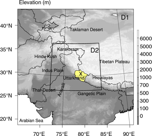
The extreme precipitation event was simulated with a two-step, one-way nesting using two domains with horizontal grid resolutions of 7 km and 2.8 km (hereafter D1 and D2 respectively, see Fig. 2). The resolution of the D2 domain is still quite coarse and does not fully resolve the complex topography of this region, which we acknowledge as one of the limitations of this study. The outermost domain D1 encompasses the Hindu Kush Himalayan region, the Tibetan Plateau, the Thar Desert in the south and the Taklamakan Desert in the north, and some of the major river basins (Amu Darya, Tarim in the north, and Indus and Ganges on the south). The Hindu Kush Himalayan range extends over more than 3500 km from Afghanistan in the west to Myanmar in the east, along with the Tibetan Plateau in the north and the Indo-Gangetic Plain in the south, all exerting a strong control on the synoptic weather systems in the region. The initial and boundary condition for the larger D1 domain was interpolated from the GME analysis. The D1 domain was initialised at 0000 UTC 11 September 2012 and integrated for 94 hours until 2200 UTC 14 September 2012, with a model time step of 60 seconds. The Tiedtke convective scheme parameterisation was used for deep convection. The hindcast simulation output from the D1 domain was then used as the initial and boundary conditions for the smaller D2 domain. The D2 domain encompasses the northwestern part of the Indo-Gangetic Plain, the western indentation of the Himalayas and the Uttarakhand state (masked region in Fig. 2), which is the focus area of this study. The D2 domain was initialised at 0000 UTC 12 September 2012, and integrated for 70 hours, till 2100 UTC 14 September 2012, with a model time step of 20 seconds. The deep convection parameterisation was turned off for the D2 simulations, because on this resolution it is assumed that deep convection can be resolved explicitly by the model, in contrast to shallow convection for which the subgrid-scale parameterisation was switched on. The latter handles the vertical redistribution of heat and moisture by shallow convection, but does not impact precipitation generation directly. This setup is also the operational configuration for COSMO-DE at DWD.

Fig. 2 Model domain and orography (m) with relevant geographical features. D1 and D2 have horizontal model resolutions of 7 km and 2.8 km respectively. The Ukhimath station in Uttarakhand state (masked in yellow), where the flood event took place is marked with X (30.30°N, 79.25°E).

4. Results and discussion

4.1. Spatial and temporal distribution of precipitation

The spatial pattern of the 3B42 (V7) daily precipitation product from the TRMM satellite was compared with the model results for the smaller D2 domain. Over the Uttarakhand state, the model underestimates the spatial extent of the daily-accumulated precipitation when compared to the TRMM product; both data show, however, consistent spatial patterns for the precipitation maxima along the lower and upper foothills of the Himalayas as outlined by the two boxes (see comparison between Fig. 3a and b). This qualitative agreement makes us confident to further investigate the mechanisms behind the extreme rainfall event based on the model results. Figure 3c shows the modelled daily-accumulated precipitation over this area along with its complex topography at the 2.8 km resolution of the D2 domain. Ukhimath Tehsil is located on the protruding foothills of the Himalayas with adjacent dissected valleys on either side, which open up towards the southwest. The simulated maximum daily accumulated rainfall for the event sums up to over 200 mm/d over the location ‘o’, which is somewhat to the east of Ukhimath Tehsil (see Fig. 3d). The model does not produce any extreme precipitation in Ukhimath Tehsil itself, while the maximum precipitation is consistent with the TRMM data over the region. In the model rainfall starts around 1700 UTC (+0530 LT) and reaches its maximum during the midnight of 13 September 2012. In the following sections, we will focus on the meteorological conditions and the potential mechanism behind this rainfall event based on the model and aided by the observations.

Fig. 3 (a) Daily accumulated precipitation on 13 September 2012 from TRMM 3B42 data; (b) Daily accumulated precipitation on 13 September 2012 simulated using COSMO (D2 domain). Two bands of precipitation are outlined by frames [in (a) and (b)] along with the borders of Uttarakhand state. (c) Zoomed modelled accumulated precipitation with the local topography at the resolution of the D2 model domain (2.8 km). The topography contour interval is 500 m reaching from 2000 to 6000 m elevation. (d) Time-series of accumulated precipitation at location marked ‘o’ (red) and the surrounding grid cells (grey), starting 12 September 2012. The precipitation accumulation shown in the spatial distributions is derived from 0000 UTC to 2330 UTC.

4.2. Meteorological setting before and during the rainfall event

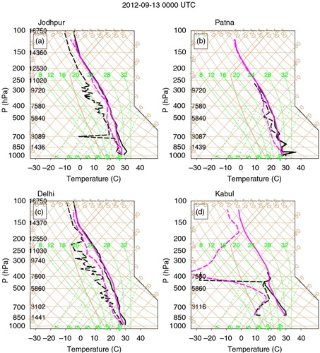
A low pressure system, which extends to mid-tropospheric levels (up to 650 hPa) along the central part of the Gangetic Plain, acts like a conveyor belt driving moist air originating from the Bay of Bengal and the Arabian Sea across central India at lower levels along the Gangetic Plain towards north-western India. Figure 4 depicts the synoptic conditions for the simulation period before the storm event at 13 September 0000 UTC for the D1 domain. The low-level monsoonal flow to the Indian subcontinent bifurcates along the Aravalli range [also referred to as the hydrometeorological dryline by Chiao and Barros (2007)] into a southerly flow traversing the Indus Plain and a westerly flow traversing across central India (Fig. 4a). The cyclonic circulation contributes to a strong easterly component at the foothills of the Himalayas, transporting moist air towards the western indentation, where it decelerates as it meets the southerly flow traversing the Indus Plain. The convergence of the low-level easterly wind with the southerly near-surface transport of moist air directly from the Arabian Sea results in a higher water vapour mixing ratio in the upper Indus Plain and the Gangetic Plain compared to the surrounding region. The low-level easterly component, which extends up to 750 hPa, also transports moist air towards the Uttarakhand state (Fig. 4b and c). At 750 hPa, warm and dry air flows north-easterly from Afghanistan towards the Indus Plain, which finally outflows into the Arabian Sea (Fig. 4b). At mid-level (500 hPa), a dry north-westerly flow prevails over the Uttarakhand state (Fig. 4d). Moist air is transported in the lower atmosphere in a sort of conveyor belt along Jodhpur, Patna, Delhi and Patiala, before decelerating at the western indentation. From mid to upper levels, the westerly flow passes through Kabul towards the study area. Observations of the vertical structure of the atmosphere were available from radiosondes launched at 13 September 0000 UTC over Jodhpur, Patna, Delhi and Kabul and are compared in Fig. 5 with the simulated thermodynamic structure of the atmosphere at these locations. Modelled (in brackets) and measured values of precipitable water compare well at Jodhpur, Delhi and Kabul [59 (64) mm, 81 (64) mm, 61 (59) mm and 20 (17) mm] except in Patna [81 (64) mm], where the model under-estimates the precipitable water. The temperature profiles are wet-adiabatic for Jodhpur (Fig. 5a), Patna (Fig. 5b) and Delhi (Fig. 5c), which lie on the moist side of the monsoon region accompanied with high precipitable water content. In general, the vertical profiles of temperature and dew point are well captured by the model. However, the model tends to be moister above 500 hPa in Jodhpur and misses the thin dry layer of air around 700 hPa. A sounding profile extracted from the model further westward (by 2 degrees, not shown here) did capture this thin dry layer with drier air atop. This suggests that the radiosonde might have drifted slightly westward due to the outflow at this level (see Fig. 4c), and hence shows drier air compared to the model. At Patna, the model tends to be relatively dry below 700 hPa causing the underestimation of precipitable water. The model also misses the low-level inversion present in Jodhpur and Patna. On the dry side, in Kabul, both temperature and dew point are well captured by the model with dry air around 700–800 hPa (also observed westward near Jodhpur), a thin layer of relatively moist air at 600 hPa, and very dry air above 400 hPa. This is consistent with similar observations made by Medina et al. (2010) near the western indentation, suggesting the presence of mid-level moist monsoonal air mass between the two sources of dry air.

Fig. 4 Simulated atmospheric state variables for the D1 domain on 13 September 0:00 UTC: air temperature (K, colour shading), wind vectors (m/s, see scale in d) and water vapour mixing ratio (g/kg, green contour lines) at pressure levels a) 925 hPa, b) 750 hPa, c) 825 hPa and d) 500 hPa. The ‘x’ mark represents the Ukhimath town. The location of radiosonde stations over the domain in Jodhpur (J), Patna (P1), Delhi (D), Patiala (P2) and Kabul (K) are also marked.

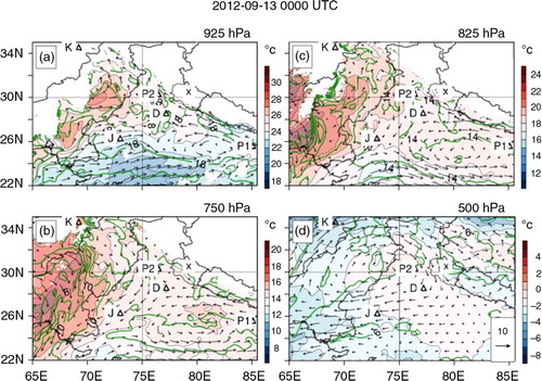
Fig. 5 Simulated (magenta) and measured (black) atmospheric soundings on 13 September 0000 UTC at (a) Jodhpur, (b) Patna, (c) Delhi and (d) Kabul. The model soundings were extracted from D1 domain for grid columns nearest to the sounding locations.

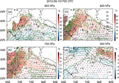
During storm evolution, the low-level south-westerly flow from the Arabian Sea intensifies, whereas the easterly flow along the foothills of the Himalaya weakens (Fig. 6a). Below 925 hPa, the southerly flow along the Indus Plain strengthens and widens reaching up to the western edge of the Uttarakhand state, where it veers northward. At 825 hPa, the easterly flow along the foothills of the Himalayas also starts weakening after 0600 UTC and retreats backward with the development of a warmer north-westerly flow, accompanied by the outflow of warm dry air over the Indus Plain from Afghanistan and the strengthening of the north-westerly flow over the upper Indus at 750 hPa (Fig. 6b and c). At 500 hPa, the dry north-westerly flow over the Uttarakhand state also strengthens gradually.

Fig. 6 Simulated atmospheric state variables for the D1 domain on 13 September 1700 UTC: air temperature (K, colour shading), wind vectors (m/s, see scale in d) and water vapour mixing ratio (g/kg, green contours) at pressure levels a) 925 hPa, b) 750 hPa, c) 825 hPa and d) 500 hPa. The ‘x’ mark represents the Ukhimath town. The location of radiosonde stations over the domain in Jodhpur (J), Patna (P1), Delhi (D), Patiala (P2) and Kabul (K) are also marked.

4.3. Mechanism of convection initiation at Ukhimath Tehsil

The orography near Ukhimath Tehsil consists of ridges protruding from the foothills of the Himalayas with dissected valleys on either side. The circulation generated by this topography is found to influence convection evolution for this particular event. Figure 7a shows the convergence of the moist easterly wind (from the Gangetic Plain, see Fig. 4b) towards the valley recesses, uphill and downhill of Ukhimath Tehsil. The convergence of moisture along these foothills increases the water vapour mixing ratio and the equivalent potential temperature of the air entering the valley recesses, where the flow is blocked. Accordingly, the boundary layer is moistened in these pockets during the daytime hours.

Fig. 7 (a) Simulated atmospheric state variables for the D2 domain on 13 September 0000 UTC: equivalent potential temperature (K, colour shading), wind vectors (m/s) and water vapour mixing ratio (g/kg, green contours) at 825 hPa. The ‘x’ and ‘o’ marks represents the Ukhimath town and the location of maximum precipitation, respectively. (b) Vertical profiles of averaged U and V wind components, gradients of potential temperature and equivalent potential temperature, along the cross-section AA’ in the valley upstream of Ukhimath town (indicated by Δ). (c) Cross-section AA’ of equivalent potential temperature (K, colour shading), wind vectors (m/s) and potential temperature (K, black contours).

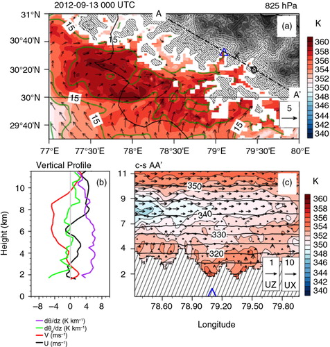
To examine the vertical structure of the atmosphere before convection initiation, a vertical cross-section AA’ oriented along the storm evolution path showing wind vectors, equivalent potential temperature (θ _e ) and potential temperature (θ) is presented in Fig. 7c. Along this cross-section, θ _e decreases with height up to 8 km, indicating a potentially unstable layer, while θ increases with height everywhere. This setting is similar to the situation presented by Medina et al. (2010) for a deep convective event near the western indentation during the monsoon season. The vertical structure of the atmosphere in the valley recesses upstream of Ukhimath Tehsil (Δ) is even better illustrated by the averaged vertical profiles of wind speed and vertical gradients of θ and θ _e (Fig. 7b). At the levels below the ridges, there is a steady up-valley flow (positive V wind), which advects moist air and increases the potential instability of the blocked air mass below. The Froude number (Fr) of this low-level air mass was also calculated to check, if this flow is blocked/unblocked by the protruding hill (Ukhimath Tehsil, 850 m in elevation from the valley). The Froude number is calculated as Fr=(U/NH), where U is the upstream wind speed perpendicular to the hill, N is the Brunt–Väisälä frequency and H is the height of the hill. Fr was estimated to be less than 1, indicating that this low-level air mass is blocked. On the other hand, the maxima in the vertical gradient of θ above the ridges and a minima in the vertical gradient of θ _e below the ridges suggests the presence of strong stable layer above the ridge, which acts as a lid inhibiting convection. The wind changes direction above the ridges and becomes weak north-westerly with relatively high wind speeds above 6 km, which advects dry air over the region.

The potential instability of the air mass below the lid increases as a result of persistent influx of moist air and diurnal heating. After 0800 UTC (+0545 LT), the south-easterly wind at 825 hPa towards the valley recess from the Gangetic Plain decelerates along with the strengthening of the mid-level north-westerly flow from the western indentation. Figure 8a shows the change in wind direction at 850 hPa from south-easterly to north-westerly from 0000 to 1400 UTC. The strengthening of north-westerly winds from 4 to 6 km is clearly visible in Fig. 8b and c, which enhances the advection of dry air at the lower levels and increases the instability of the air mass below. In consequence, the development of a strong vertical wind shear above the ridge (Fig. 8b) pushes the potentially unstable layer above the protruding ridge of Ukhimath Tehsil (Fig. 8c) and produces the necessary uplift to overcome the lid and trigger convection. The effect of vertical wind shear is also clearly visible in the slope of the contours of θ _e in Fig. 8c. The vertical gradient of θ _e has a minimum around 4.5 km, along with the maximum of the north-westerly wind speed and a local minimum in the vertical gradient of θ at 1400 UTC, when the convection is triggered (see Fig. 8b and c).

Fig. 8 (a) Simulated atmospheric state variables for the D2 domain on 13 September 1400 UTC: equivalent potential temperature (K, colour shading), wind vectors (m/s) and water vapour mixing ratio (g/kg, green contours) at 825 hPa. The ‘x’ and ‘o’ marks represent the Ukhimath town and the location of maximum precipitation, respectively. (b) Vertical profiles of averaged U and V winds, gradients of potential temperature and equivalent potential temperature, along the cross-section AA’ in the valley upstream of Ukhimath town (Δ). (c) Cross-section AA’ of equivalent potential temperature (K, colour shading), wind vectors (m/s) and potential temperature (K, black contours).

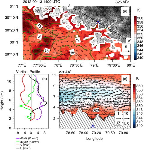
The convergence of low-level moist air in the valley upstream to Ukhimath Tehsil and the development of a strong north-westerly dry wind above the ridges, pushes the potentially unstable air mass eastward over the protruding foothills of the Himalayas, which generates the necessary uplift to erode the lid and trigger convection. This orographic lifting of potentially unstable air acts as a trigger mechanism for deep convection over this region, which is consistent with and corroborates the findings from previous studies (Sawyer, 1947; Houze et al., 2007; Medina et al., 2010; Houze, 2012).

4.4. Microphysics of the convective storm

The mid-level north-westerly wind advects the potentially unstable air mass above the foothills in Ukhimath Tehsil after triggering shallow convection and generates a precipitating system spreading out to approximately 40 km in the horizontal at upper levels (along cross-section AA’), with cloud tops near the freezing level (near 5.2 km). Figure 9a shows the spatial extent of the vertically integrated rain-water mixing ratio (qr) superimposed on the 2.8 km resolution topography and 500 hPa wind vectors at 1515 UTC. This shallow convective cloud system is already well developed around 1400 UTC above Ukhimath Tehsil and precipitates via warm rainfall processes as it crosses this barrier (Fig. 9b, snapshot of the hydrometeors at 1515 UTC). As the updraft continues while the cloud system is advected over the barrier, graupel formation initiates at 6 km height by freezing raindrops. Figure 9b shows the average vertical hydrometeor profiles taken at the location with maximum vertically integrated rainwater content, along AA’ (Δ). The peak cloud-water mixing ratio (qc) of around 2.5 g/kg is located near the freezing level and decreases sharply above. The rain-water mixing ratio increases gradually from this level downwards, reaching a maximum of 1 g/kg near the surface. The raindrop formation accelerates after 1445 UTC by the collision-coalescence mechanism. The cross-section also shows the presence of graupel above the freezing level in the early formation phase (just barely visible in the figure at 6 km). Also, a thin layer of cirrus clouds was present at a height of 14 km with snow and ice mixing ratios (qs and qi) in the order of less 0.001 g/kg (not visible in Fig. 9c due to contour levels). This modelled height of cirrus clouds over the region is consistent with the vertical frequency distribution of observed cirrus clouds during JJAS over India (Subrahmanyam and Kumar, 2013). At mid-level, the strong north-westerly wind advects the precipitating cloud system further eastward of Ukhimath Tehsil. This system survives while advected from one ridgeline to the other, taps the low-level moisture in the valley and reaches the foothills of the adjacent ridgeline at 1645 UTC. During this propagation, the cloud top height increases gradually from 6 to 8 km, with snow and ice particle formation above 6 km, which contribute to the increase in graupel mixing ratio (qg) by riming, while the qc and qr profiles remain quasi-stationary. As this system crosses the second ridgeline, the cloud top of the convective system reaches the upper level cirrus clouds and triggers a strong updraft at the upper level leading to deep convection with the cloud top height reaching 14 km at 1815 UTC (not shown). Figure 10a shows the vertically integrated rain-water mixing ratio at 1845 UTC, which outlines the horizontal extent of raindrop formation with peak concentrations over the region (‘o’) where maximum precipitation was simulated. The vertical hydrometeor profile shows high qg values extending from 5 to 13 km with peak mixing ratios of 3.5 g/kg around 6 km (Fig. 10b). Strong updrafts also transport cloud and rain drops up to 11 km, where they exist as super-cooled drops. Snow and ice particles extend from 6 to 14 km, with qs peaking nearly to 1 g/kg at 10.5 km and qi peaking to 0.5 g/kg at 13 km height. The graupel-dominated microphysical process is primarily due to riming of snow and freezing of raindrops or freezing of raindrops by collision with ice particles. Below the melting level, raindrop formation is intensified by melting of graupel with peak qr reaching 2 g/kg. At this time, a second shallow convective system develops over the ridge line of Ukhimath Tehsil, which also propagates eastwards and eventually dissipates along with the deep convective storm by 2245 UTC.

Fig. 9 (a) Simulated atmospheric state variables for the D2 domain on 13 September 1515 UTC: vertically integrated rain-water mixing ratio (g/kg, colour shading) and wind vectors (m/s) at 500 hPa. The ‘x’ and ‘o’ marks represent the Ukhimath town and the location of maximum precipitation, respectively. (b) Averaged vertical profiles of hydrometeors at precipitation maximum (Δ), along the cross-section AA’. (c) Cross-section AA’ of hydrometeors (qr in colour shading, qc, qi, qg, qs in solid lines from 0.2 to 2.4 g/kg at intervals of 0.4 g/kg), wind vectors and temperature (black contours, showing the melting level). [qx refers to mixing ratio of different hydrometeors, with x being cloud water (qc), cloud ice (qi), graupel (qg), snow (qs) and rain (qr)].

Fig. 10 (a) Simulated atmospheric state variables for the D2 domain on 13 September 1845 UTC: vertically integrated rainwater mixing ratio (g/kg, colour shading) and wind vectors (m/s) at 500 hPa. The ‘x’ and ‘o’ marks represent the Ukhimath town and the location of maximum precipitation, respectively. (b) Averaged vertical profile of hydrometeors at precipitation maximum (Δ), along the cross-section AA’. (c) Cross-section AA’ of hydrometeors (qr in colour shading, qc, qi, qg, qs in solid lines from 0.2 to 2.4 g/kg at intervals of 0.4 g/kg), wind vectors and temperature (black contours, showing the melting level). [qx refers to mixing ratio of different hydrometeors, with x being cloud water (qc), cloud ice (qi), graupel (qg), snow (qs) and rain (qr)].

This convective rainfall event simulated for the D2 domain, lasted for almost 8 hours. Mid-level advection and graupel formation played an important role in the evolution of the storm and the spatial distribution of the rainfall. Similar findings were presented as a conceptual model by Medina and Houze (2003) for the Mesoscale Alpine Programme (MAP) storms, where the rapid lifting of low-level moist air above the terrain enhanced graupel formation with large enough fall velocities to fall out quickly (i.e. release precipitation), which is also coined as ‘cloudburst’ in Indian meteorological parlance.

5. Conclusions

Our analysis of daily maximum rainfall from TRMM data over Uttarakhand state shows that extreme rainfall events exceeding 200 mm/d are not uncommon in this region given an exceedance probability for 200 mm/d rainfall for the JJAS period of around 1.6%. Given the uncertainty of TRMM data over higher elevations (Barros et al., 2000; Iguchi et al., 2009; Rasmussen et al., 2013), this exceedance probability could be an underestimate. One event with such an extreme rainfall, which occurred on the midnight of 13 September 2012 and caused flash flood and landslide in Uttarakhand state, is examined in detail in this study using the operational weather forecast model COSMO in a convection permitting configuration. The modelled results are compared with available satellite retrievals and radiosonde observations. Satellite-retrieved daily-accumulated precipitation from TRMM compares well with the modelled structure of maximum precipitation over the region. The radiosonde observations over Jodhpur, Patna, Delhi and Kabul were also compared with the model simulations near these locations. In general, the vertical profiles of temperature and dew point are well captured by the model and add confidence on the modelled results for an in-depth investigation of the mechanism of the extreme rainfall event.

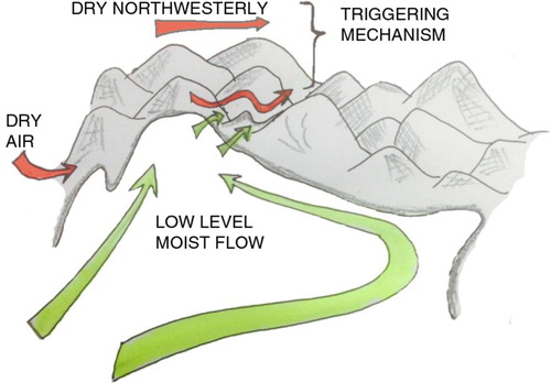
The mechanisms leading to this extreme rainfall event based on the numerical model analysis is illustrated in Fig. 11 and summarised below:

1. A low pressure system along the central part of the Gangetic Plain produced a low-level easterly wind along the Gangetic Plain adjacent to the foothills of the Himalayas, which transports moist air towards the north-western part of India and to the inner valley recesses along the path including the valleys adjacent to Ukhimath Tehsil. This moist easterly flow meets the warm and moist southerly flow coming directly from the Arabian Sea at the western indentation resulting in a convergence of moisture.

2. This moisture transport towards the valley recesses increases the potential instability of the air, which is capped by an inversion layer located above the ridgeline, during the daytime.

3. The retreat of the low-level easterly wind with the strengthening of the north-westerly flow, and the development of mid-level wind shear above the ridge line, advects this potential unstable layer above the protruding ridge of Ukhimath Tehsil, triggering shallow convection. This precipitating convective system moves eastward along another fold of valley and ridge, triggering deep convection, which produced high rainfall over the region by intensification of graupel formation with large enough fall velocities to fall out quickly as precipitation.

Fig. 11 Schematic of the meteorological setting and suggested mechanism for the occurrence of extreme rainfall event in Uttarakhand.

This study suggests a possible mechanism for extreme rainfall event generation over this region, which confirms and corroborates the earlier findings of Houze et al. (2007) and Medina et al. (2010) over the western indentation of the Himalayas. It also demonstrates that mesoscale models like COSMO can be used to simulate such events. However, more modelling studies with multiple events and radar observations over the region are essential to better understand the full spectrum of these deep convective events over the region.

6. Acknowledgements

This work was funded by SFB/TR32 (www.tr32.de), ‘Patterns in Soil–Vegetation–Atmosphere Systems: Monitoring, Modeling, and Data-Assimilation’, funded by the Deutsche Forschungsgemeinschaft (DFG). The second author was supported by DAAD for this work. We thank the Deutscher Wetterdienst (DWD) for the COSMO and GME analysis data and the COSMO model code. The post-processing of COSMO output was done using the NCAR Command language version 6.1.2 (NCAR 2013). The TRMM precipitation data used in this study were downloaded with the Giovanni online data system, developed and maintained by the NASA GES DISC.

References

- Baldauf M. , Seifert A. , Förstner J. , Majewski D. , Raschendorfer M. , co-authors . Operational convective-scale numerical weather prediction with the COSMO model: description and sensitivities. Mon. Weather Rev. 2011; 139: 3887–3905. 10.1175/MWR-D-10-05013.1.
- Barros A. P. , Joshi M. , Putkonen J. , Burbank D. W . A study of the 1999 monsoon rainfall in a mountainous region in central Nepal using TRMM products and rain gauge observations. Geophysical Research Letters. 2000; 27(22): 3683–3686.
- Barros A. P. , Kim G. , Williams E. , Nesbitt S. W . Probing orographic controls in the Himalayas during the monsoon using satellite imagery. Nat. Hazards Earth Syst. Sci. 2004; 4(1): 29–51.
- Blackadar A. K . The vertical distribution of wind and turbulent exchange in neutral atmosphere. J. Geophys. Res. 1962; 67: 3095–3102. 10.1029/JZ067i008p03095.
- Caracena F. , Maddox R. A. , Hoxit L. R. , Chappell C. F . Mesoanalysis of the Big Thompson storm. Mon. Weather Rev. 1979; 107(1): 1–17.
- Chiao S. , Barros A. P . A numerical study of the hydrometeorological dryline in northwest India during the monsoon. J. Meteorol. Soc. Jpn. 2007; 85: 337–361.
- Das S. , Ashrit R. , Moncrieff M. W . Simulation of a Himalayan cloudburst event. J. Earth Syst. Sci. 2006; 115(3): 299–313.
- Das S. , Singh S. V. , Rajagopal E. N. , Gall R . Mesoscale modeling for mountain weather forecasting over the Himalayas. Bull. Am. Meteorol. Soc. 2003; 84(9): 1237–1244.
- Doms G . A Scheme for Monotonic Numerical Diffusion in the LM. 2001. COSMO Technical Report No. 3, 24 pp. Online at: http://www.cosmo-model.org/content/model/documentation/techReports/ .
- Doms G. , Schaettler U . The Nonhydrostatic Limited-Area Model LM–Part I: Dynamics and Mumerics. 2002. Scientific Documentation, DeutscherWetterdienst, Offenbach, Germany, 140 pp. Online at: http://www.cosmo-model.org .
- Doms G. , Förstner J. , Heise E. , Herzog D. , Mironov M. , co-authors . A Description of the Nonhydrostatic Regional Model LM. Part II: physical Parameterization. 2011; Deutscher Wetterdienst. Online at: http://www.cosmo-model.org .
- Findlater J . A major low-level air current near the Indian Ocean during the northern summer. Q. J. Roy. Meteorol. Soc. 1969; 95(404): 362–380.
- Houze R. A . Orographic effects on precipitating clouds. Rev. Geophys. 2012; 50(1): 10.1029/2011RG000365.
- Houze R. A. Jr. , Rasmussen K. L. , Medina S. , Brodzik S. R. , Romatschke U . Anomalous atmospheric events leading to the summer 2010 floods in Pakistan. Bull. Am. Meteorol. Soc. 2011; 92(3): 291–298.
- Houze R. A. Jr. , Wilton D. C. , Smull B. F . Monsoon convection in the Himalayan region as seen by the TRMM Precipitation Radar. Q. J. Roy. Meteorol. Soc. 2007; 133(627): 1389–1411.
- Huffman G. J. , Bolvin D. T. , Nelkin E. J. , Wolff D. B. , Adler R. F. , co-authors . The TRMM multisatellite precipitation analysis (TMPA): quasi-global, multiyear, combined-sensor precipitation estimates at fine scales. J. Hydrometeorol. 2007; 8(1): 38–55.
- Iguchi T. , Kozu T. , Kwiatkowski J. , Meneghini R. , Awaka J. , co-authors . Uncertainties in the rain profiling algorithm for the TRMM precipitation radar. J. Meteorol. Soc. Jpn. 2009; 87A: 1–30.
- Lin Y.-L. , Farley R. D. , Orville H . Bulk parameterization of the snow field in a cloud model. J. Clim. Appl. Meteorol. 1983; 22: 1065–1092. 10.1175/1520-0450(1983)022,1065:BPOTSF.2.0.CO;2.
- Maddox R. A. , Hoxit L. R. , Chappell C. F. , Caracena F . Comparison of meteorological aspects of the Big Thompson and Rapid City flash floods. Mon. Weather Rev. 1978; 106(3): 375–389.
- Majewski D. , Liermann D. , Prohl P. , Ritter B. , Buchhold M. , co-authors . The operational global icosahedral-hexagonal gridpoint model GME: description and high-resolution tests. Mon. Weather Rev. 2002; 130(2): 319–338.
- Matsueda M . Predictability of Euro-Russian blocking in summer of 2010. Geophys. Res. Lett. 2011; 38: 6.
- Medina S. , Houze R. A . Air motions and precipitation growth in Alpine storms. Q. J. Roy. Meteorol. Soc. 2003; 129(588): 345–371.
- Medina S. , Houze R. A. , Kumar A. , Niyogi D . Summer monsoon convection in the Himalayan region: terrain and land cover effects. Q. J. Roy. Meteorol. Soc. 2010; 136(648): 593–616.
- Mellor G. L. , Yamada T . Development of a turbulence closure model for geophysical fluid problems. Rev. Geophys. Space Phys. 1982; 20: 851–875. 10.1029/RG020i004p00851.
- Nair U. S. , Hjelmfelt M. R. , Pielke R. A., Sr . Numerical simulation of the 9–10 June 1972 Black Hills storm using CSU RAMS. Mon. Weather Rev. 1997; 125(8): 1753–1766.
- Nandargi S. , Dhar O. N . Extreme rainstorm events over the Northwest Himalayas during 1875–2010. J. Hydrometeorol. 2012; 13(4): 1383–1388.
- NCAR. Boulder, Colorado: UCAR/NCAR/CISL/TDD. The NCAR Command Language, version 6.1.2. 2013. 10.5065/D6WD3XH5.
- Raschendorfer M . The new turbulence parameterization of LM. COSMO Newsletter. 2001. Vol. 1, Consortium for small-scale modeling, pp. 89–97. Online at: http://www.cosmo-model.org/content/model/documentation/newsLetters/newsLetter01/newsLetter_01.pdf .
- Rasmussen K. L. , Choi S. L. , Zuluaga M. D. , Houze R. A., Jr . TRMM precipitation bias in extreme storms in South America. Geophys. Res. Lett. 2013; 40: 3457–3461. 10.1002/grl.50651.
- Rasmussen K. L. , Hill A. J. , Toma V. E. , Zuluaga M. D. , Webster P. J. , co-authors . Multiscale analysis of three consecutive years of anomalous flooding in Pakistan. Q. J. Roy. Meteorol. Soc. 2014. 10.1002/qj.2433.
- Rasmussen K. L. , Houze R. A. Jr. . A flash-flooding storm at the steep edge of high terrain: disaster in the Himalayas. Bull. Am. Meteorol. Soc. 2012; 93(11): 1713–1724.
- Reinhardt T. , Seifert A . A three-category ice scheme for LMK. COSMO Newsletter. 2006. Vol. 6, Consortium for small-scale modeling, pp. 115–120. Online at: http://www.cosmo-model.org/content/model/documentation/newsLetters/newsLetter06/cnl6_reinhardt.pdf .
- Ritter B. , Geleyn J. F . A comprehensive radiation scheme for numerical weather prediction models with potential applications in climate simulations. Mon. Weather Rev. 1992; 120: 303–325. 10.1175/1520-0493(1992)120,0303:ACRSFN.2.0.CO;2.
- Romatschke U. , Houze R. A. Jr. . Characteristics of precipitating convective systems in the South Asian monsoon. J. Hydrometeorol. 2011; 12(1): 3–26.
- Romatschke U. , Medina S. , Houze R. A. Jr. . Regional, seasonal, and diurnal variations of extreme convection in the South Asian region. J. Clim. 2010; 23(2): 419–439.
- Sawyer J. S . The structure of the intertropical front over NW India during the SW monsoon. Q. J. Roy. Meteorol. Soc. 1947; 69: 346–369.
- Shrestha P. , Barros A. P . Joint spatial variability of aerosol, clouds and rainfall in the Himalayas from satellite data. Atmos. Chem. Phys. 2010; 10(17): 8305–8317.
- Steppeler J. , Doms G. , Schättler U. , Bitzer H. , Gassmann A. , co-authors . Meso-gamma scale forecasts using the nonhydrostatic model LM. Meteorol. Atmos. Phys. 2003; 82: 75–96. 10.1007/s00703-001-0592-9.
- Subrahmanyam K. V. , Kumar K. K . CloudSat observations of cloud-type distribution over the Indian summer monsoon region. Ann. Geophys. 2013; 31(7): 1155–1162.
- Tibaldi S. , Molteni F . On the operational predictability of blocking. Tellus A. 1990; 42: 343–365.
- Tiedtke M . A comprehensive mass flux scheme for cumulus parameterization in large-scale models. Mon. Weather Rev. 1989; 117: 1779–1800. 10.1175/1520-0493(1989)117,1779:ACMFSF.2.0.CO;2.
- Webster P. J. , Toma V. E. , Kim H. M . Were the 2010 Pakistan floods predictable?. Geophys. Res. Lett. 2011; 38: 04806. 10.1029/2010GL046346.
- Wicker L. J. , Skamarock W. C . Time-splitting methods for elastic models using forward time schemes. Mon. Weather Rev. 2002; 130: 2088–2097. 10.1175/1520-0493(2002)130,2088:TSMFEM.2.0.CO;2.
- Wu Y. , Raman S. , Mohanty U. C . Numerical investigation of the Somali jet interaction with the Western Ghat mountains. Pure Appl. Geophys. 1999; 154(2): 365–396.
- Zipser E. J. , Liu C. , Cecil D. J. , Nesbitt S. W. , Yorty D. P . Where are the most intense thunderstorms on Earth?. Bull. Am. Meteorol. Soc. 2006; 87(8): 1057–1071.