Assimilation of wind speed and direction observations: results from real observation experiments

Abstract

The assimilation of wind observations in the form of speed and direction (asm_sd) by the Weather Research and Forecasting Model Data Assimilation System (WRFDA) was performed using real data and employing a series of cycling assimilation experiments for a 2-week period, as a follow-up for an idealised post hoc assimilation experiment. The satellite-derived Atmospheric Motion Vectors (AMV) and surface dataset in Meteorological Assimilation Data Ingest System (MADIS) were assimilated. This new method takes into account the observation errors of both wind speed (spd) and direction (dir), and WRFDA background quality control (BKG-QC) influences the choice of wind observations, due to data conversions between (u,v) and (spd, dir). The impacts of BKG-QC, as well as the new method, on the wind analysis were analysed separately. Because the dir observational errors produced by different platforms are not known or tuned well in WRFDA, a practical method, which uses similar assimilation weights in comparative trials, was employed to estimate the spd and dir observation errors. The asm_sd produces positive impacts on analyses and short-range forecasts of spd and dir with smaller root-mean-square errors than the u,v-based system. The bias of spd analysis decreases by 54.8%. These improvements result partly from BKG-QC screening of spd and dir observations in a direct way, but mainly from the independent impact of spd (dir) data assimilation on spd (dir) analysis, which is the primary distinction from the standard WRFDA method. The potential impacts of asm_sd on precipitation forecasts were evaluated. Results demonstrate that the asm_sd is able to indirectly improve the precipitation forecasts by improving the prediction accuracies of key wind-related factors leading to precipitation (e.g. warm moist advection and frontogenesis).

• WRFDA
• observation operator
• observation error
• quality control
• variational assimilation

1. Introduction

Many types of platforms measure winds, such as surface land and marine observation networks, upper-air observation networks, aircraft and remote sensing systems. Generally, wind speed (spd) and direction (dir) are the initial products; however, the nature of wind vector measurements varies among these platforms. For example, surface winds (spd and dir) are typically measured by an anemometer on a fixed or drifting platform by a defined time-average. For aircraft-based observations, spd and dir are computed by taking the difference between the ground track vector, which includes a Global Position System (GPS)-observed speed and angle based on the latitude and longitude change between adjacent points, and the aircraft track vector, which is derived from the true air speed and the internal navigation system heading (Painting, 2003; Gao et al., 2012). Atmospheric Motion Vectors (AMV), in the forms of spd and dir, are derived from satellite imagery by tracking features over a sequence of images (Velden et al., 1998; NOAA Technical Report ; EUMETSAT report ).

The standard Weather Research and Forecasting Model Data Assimilation System (WRFDA) assimilates wind observations in the form of longitudinal and latitudinal components, conventionally abbreviated to u and v (asm_uv), which are computed from the initial observation product of spd and dir (Huang et al., 2009; Barker et al., 2012). This method is similar to other data assimilation systems, such as those described by Le Dimet and Talagrand (1986), Andersson et al. (1998) and Gustafsson et al. (2001).

In asm_uv, during the observation processing phase, which precedes assimilation, only the observational error associated with spd is used to quantify errors in u and v (Kalnay et al., 1996; Lindskog et al., 2001). This process allows the background quality control (BKG-QC) to proceed, thereby screening observations and computing a cost function based on the assimilation weight for wind-related terms.

However, the dir observational error, which can contribute uncertainty to u and v, is typically ignored. In fact, a nonlinear relationship exists between the observational errors of u and v and the errors in spd and dir. As eqs. (16) and (17) in Huang et al. (2013) indicate, the impact of dir observational error on the errors in u and v is both significant and sensitive to the background. As a result, dir observational error should not be ignored in wind data assimilation.

A new assimilation method for wind observations, which employs direct assimilation of spd and dir (asm_sd), has been developed for WRFDA (Huang et al., 2013). This method considers the dir observational error as being independent of the spd observational error, and thus the corresponding weights of spd or dir observations in the analysis are affected exclusively by the respective spd or dir observational errors.

Because it is not straightforward to build equivalent relationships among the wind measurement errors expressed in each format (Euclidean vs. radial) and the background errors of stream function/velocity potential, it is inaccurate to assume that asm_uv and asm_sd are equivalent in terms of assimilation variables due to the accuracy of transforming u and v from spd and dir. Additionally, the BKG-QC routine determines which wind observations to retain in different ways in asm_uv versus asm_sd, such that the accepted observations could vary even when the same dataset is used.

Distinct differences exist for the assimilation methods for spd and dir. In asm_sd, the spd (dir) observation and its error have an independent impact on the spd (dir) analysis. By comparison, the spd analysis is also affected by dir observations in addition to the spd observations in asm_uv. In other words, the spd analysis varies with the dir observation when the spd observation and the observational errors of u and v are constant in asm_uv, and the opposite is true for dir. These distinctions are responsible for generating different wind analyses in asm_uv compared to asm_sd.

Three key factors highlight the advantages of asm_sd real experiments:

1. BKG-QC is able to screen spd or dir observations out separately in a direct way in asm_sd. This is an advantage because there is not an effective mechanism to guarantee that u and v components computed from a spd or dir observations, that can have substantial errors, will be screened out in asm_uv.

2. The formulation of asm_sd ensures that the spd and dir analysis falls between the background and observations for both variables. In asm_uv, when u or v components point in opposite directions to the background, the asm_uv could produce a spd analysis with magnitude much smaller than what it should be. An extreme case could result in a spd of zero in the analysis regardless of spd in the background and observations (Fig. 1).

3. Unlike most surface observation stations that independently observe spd and dir, AMV and aircraft-based wind measurements are calculated from vector differences, which could lead to error correlation between dir and spd. Regardless, it is more accurate to assume that the spd observational error is independent from the dir error than to assume the same for u and v because observation error in either spd or dir affects the observational errors of both u and v simultaneously. This assumption, widely used in this type of work (e.g. Hollingsworth and Lönnberg, 1986), simplifies the observation error covariance matrix to a diagonal matrix and is more acceptable in three dimensional variational data assimilation (3D-Var) versus 4D-Var, where some successive reports from the same station could be assimilated (Jarvinen et al., 1999).

Initial comparisons between asm_uv and asm_sd by using simplified arguments and graphical illustrations were conducted by Huang et al. (2013). Although the superiority of asm_sd was demonstrated by Observation System Experiments (OSEs), the forecast model was assumed to be error free, and the ‘true’ observational errors of spd and dir were predefined instead of truly known. Additionally, observations were assimilated without any quality control. Unfortunately, none of these assumptions and conditions are valid for any experiment using real data. While this topic has never been directly addressed, the issue of estimating spd and dir observational error in relation to the BKG-QC procedures has previously been raised: how should spd and dir observation errors be calculated in practice?

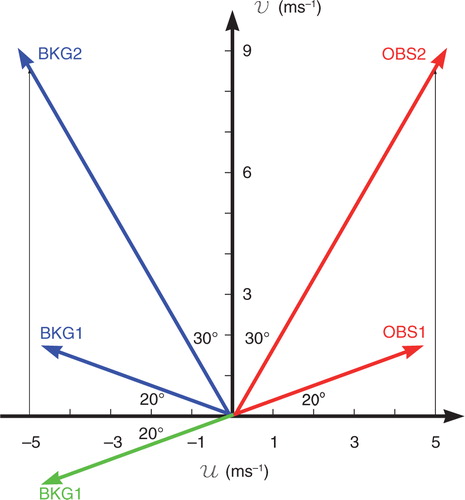
Fig. 1 Diagram of background wind vectors (BKG1 and BKG2) and the observational wind vectors (OBS1 and OBS2), used to present the differences of WRFDA background quality control procedures (BKG-QC) between asm_uv (standard assimilation method in WRFDA, assimilating wind observation in the forms of u and v components) and asm_sd (new assimilation method, assimilating wind observation in the forms of wind speed and direction).

Several studies suggest comparing an observation with an uncorrelated reference. Benjamin et al. (1999) reported on a collocation study for Aircraft Communications Addressing and Reporting System (ACARS) observations generated from aircraft with different tail numbers. Likewise, Drüe et al. (2008) estimated the observation errors of Aircraft Meteorological Data Relay (AMDAR) by considering rawinsonde observations (RAOB) as the reference. With Tropospheric Airborne Meteorological Data Reporting (TAMDAR) becoming an important part in the global observing system, Moninger et al. (2010) presented error characteristics of TAMDAR by comparing them with the Rapid Update Cycle (RUC) 1-h forecast. Although strict collocation conditions were used, these estimations actually only provide an upper bound on the combined errors of observation, reference and representativeness.

Meanwhile, the variable dir is not involved in these studies. Gao et al. (2012) calculated spd and dir observational error, independent from any reference, of TAMDAR and RAOB by matching up three types of data sources. This method is theoretically suitable for any observation type; however, it is difficult to implement that method because no other available data type has sufficient coverage to co-locate with surface data over the continental United States (CONUS). Consequently, a practical method is employed in this study to estimate the spd and dir observation errors, which are used to obtain similar assimilation weights for wind observations in asm_uv and asm_sd, as in the initial test.

Since dir observations can be screened out directly by BKG-QC in asm_sd, it is necessary and reasonable to define a critical value of dir innovation to decrease the possibility of absorbing dir observations that are grossly in error. Some studies have demonstrated that a large dir error is often correlated to light spd (Plant, 2000; Gao et al., 2012), which could be related to mesoscale variability, especially given turbulence in the boundary layer (Benjamin et al., 1999).

In the initial test, we use 90° as the dir innovation threshold in BKG-QC. Note that any dir observation with innovation exceeding 90° is not regarded by the authors as necessarily indicating the observation is erroneous. Rather, the implementation is used to emphasise the impact of dir observations on the spd analysis in asm_uv in the situation that the vectors of background and observation are located in different quadrants. Although any dir innovation except zero could lead to this situation, it is assured to be rejected by restricting dir innovation to <90°.

Unless there is equivalency of the dir between observation and background, when assuming equal assimilation weights for wind observations in asm_uv and asm_sd, the scalar nature of spd generates a smaller spd innovation in asm_sd than the spd innovation converted from u and v innovations in asm_uv. Therefore, to avoid using spd observations with a bias towards larger spd innovations, the magnitude of the allowed spd innovation should be reduced in asm_sd, as compared to asm_uv.

Given that wind observations from different platforms with unique error characteristics (e.g. Plant, 2000; Drüe et al., 2008; Gao et al., 2012) are being used even when dir observation errors are rarely known, the varied nature of these input sources could increase the uncertainty of assimilation results.

This study is primarily designed to evaluate the performance of asm_sd in assimilating the satellite-derived AMV and surface-based dataset in Meteorological Assimilation Data Ingest System (MADIS), which provides the best coverage over CONUS.

When using an observation that is already assimilated into the background for verification reference, the obtained analysis correlates with the observation; thus, the verification for experiments may be biased because aliasing will inherently favour the experiment with larger assimilation weights for observations. This study evaluates model analyses and short-range forecasts against RAOB, which were not used in the assimilation, and are thus fully independent from analyses and forecasts. Finally, a precipitation event that occurred during the experimental period was chosen to further explore the indirect impacts of asm_sd on precipitation prediction in the full-cycle assimilation scheme. The precipitation reference is National Centers for Environmental Prediction (NCEP) Stage IV analysis with a resolution of 4 km (Lin and Mitchell, 2005).

The remainder of the paper is arranged as follows. In Section 2, we provide an overview of the new method and discuss distinctions concerning BKG-QC between asm_uv and asm_sd by using two cases. Section 3 describes the model configuration, the estimation of observation errors of spd and dir, and experiment design. The statistical results of evaluation and a precipitation case study are presented in Section 4. Finally, conclusions and an outlook for future research are provided in Section 5.

2. BKG-QC in the assimilation of wind speed and direction

The formulation of asm_sd apart from the details of BKG-QC is described in Huang et al. (2013). In brief, the variables related to wind in the innovation vector, observation error covariance and observation operators that participate in the cost function [Huang et al., 2013; eq. (1)] are transformed from u and v in asm_uv to spd and dir in asm_sd. Thus, the observation error covariance matrix R _{asm_sd} in asm_sd has variances of observation errors of spd and dir on the diagonal, replacing u and v in R _{asm_uv}:1 ${\mathbf{R}}_{\text{asm}\_\text{uv}}=\left(\begin{array}{cccc}\ddots & 0& 0& 0\\ 0& {\sigma }_u^2& 0& 0\\ 0& 0& {\sigma }_v^2& 0\\ 0& 0& 0& \ddots \end{array}\right)\Rightarrow {\mathbf{R}}_{\text{asm}\_\text{sd}}=\left(\begin{array}{cccc}\ddots & 0& 0& 0\\ 0& {\sigma }_{spd}^2& 0& 0\\ 0& 0& {\sigma }_{dir}^2& 0\\ 0& 0& 0& \ddots \end{array}\right)$1 In this study, the observation errors of u and v in asm_uv, σ _u and σ _v , employ the default errors defined in the WRFDA error table (Kalnay et al., 1996), and the observation errors of spd and dir, σ _spd and σ _dir , will be estimated in the next section.

The basic procedures of quality control, which are performed on observations before assimilation, include assessing vertical consistency (super adiabatic and wind shear checks) and a dry convective adjustment. Additionally, like in most data assimilation systems, the innovation and observation error are used in BKG-QC in WRFDA to determine data retention. Any observation y _i is rejected if2 $d_i>n\times {\sigma }_i$2 where d _i is the innovation (i.e. observation y _i minus the corresponding background), σ _i is the error for observation y _i , and n represents a fixed multiple of the observation error, which is set to 5 as default in WRFDA.

As stated above, asm_sd can generate a smaller spd innovation than asm_uv due to the scalar nature of spd under certain conditions. This conclusion can be explained similarly by Huang et al. (2013; Fig. 8), where u and v differences from reference are roughly 1.6 times of spd difference. Based on the statistics, n is defined as 3 for spd BKG-QC in asm_sd for this study.

In asm_sd, y _i and σ _i denote the spd or dir observation and its observational error, respectively. Thus, a spd or dir observation can be retained or directly screened out. However, eq. (2) is not able to effectively block a spd or dir observation grossly in error from being assimilated in asm_uv, because u and v innovations are not necessary for assessing eq. (2) when spd and dir innovations meet the requirements. Two cases illustrated in Fig. 1 present the differences in BKG-QC between asm_uv and asm_sd, where the spd observations and backgrounds are assumed to be equal for simplification, and spd observation error is defined as 2 ms⁻¹.

In case 1 (OBS1 and blue BKG1), a dir component of OBS1 with innovation exceeding 90° is rejected and only the spd component is assimilated into the analysis in asm_sd. By comparison, the u component of OBS1 is contaminated by the dir component being grossly in error, and even with an innovation score of 9.0 ms⁻¹ (less than 5x the observation error, 10.0 ms⁻¹), it is still assimilated into asm_uv. The assimilation produces a spd analysis falling outside the interval defined by the background and observation, as in Huang et al. (2013; Fig. 1).

In extreme situations, when assuming the equality of observation error and background error, the OBS1 and green BKG1 (with magnitudes ~4.7 ms⁻¹) will produce zero spd analysis in asm_uv. It would be preferable for a reasonable spd analysis to maintain a magnitude close to both the background and observation (~4.7 ms⁻¹). Based on this case, there will always be a set of u and v observation errors leading to a spd analysis of zero in asm_uv when the dir innovation exceeds 90°, regardless of the magnitude of spd in background and observation.

In case 2, OBS2 is a good observation to be used in asm_sd; however, the u component of OBS2 is rejected in asm_uv due to the u innovation being larger than 10 ms⁻¹. Thus, the positive impacts of the good observation are lost in asm_uv. Although these counterexamples cannot lead to a conclusion that BKG-QC in asm_sd is uniformly superior to that of asm_uv, the former is more effective and reasonable than the latter based on these two simple cases. Typically, situations like case 1 are often observed near the surface, and situations similar to case 2 more frequently occur at higher altitudes.

3. Experimental framework

3.1. Model configuration

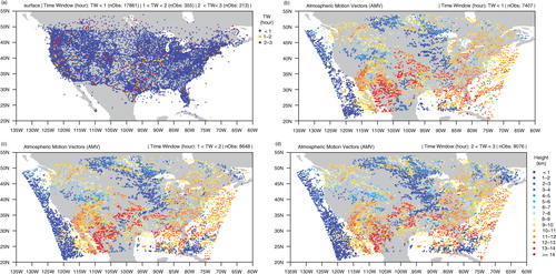
The Weather Research and Forecasting (WRF) model (Skamarock et al., 2008) was run with 15-km grid spacing on a 334×223 horizontal grid domain covering the CONUS and surrounding oceans (Fig. 2), using 37 vertical levels laid out with the model top at 50 hPa. The MADIS AMV and surface (including temperature, relative humidity and surface pressure in addition to spd and dir) datasets are used in this study. The experimental domain is shown in Fig. 2, as an example of the observation distributions on 0000 UTC 1 August 2013. Compared with the average distribution of AMV by time window, most surface data are centred ±1 h around the analysis time, which improves the accuracy of assimilation by narrowing the time gap between the background and observations.

Fig. 2 The experimental domain and the spatial and temporal distributions of MADIS surface (a) and satellite-derived Atmospheric Motion Vectors (AMV) observations (b–d) at 0000 UTC 1 August 2013 with the time window of ±3 h. The observation count (nObs) is shown by time window on top. The time window is denoted by colours in (a), and the vertical height is denoted by colours in (b–d).

The experimental window begins at 0000 UTC 1 August 2013 and lasts for 2 weeks. The assimilation employs 3D-Var, and runs four times at 0000, 0600, 1200 and 1800 UTC per day with 6-h cycling (i.e. the 6-h forecast initialised from the previous analysis is considered as background). The time window of the assimilation was 3 h on either side of the analysis time. The National Meteorological Center (NMC) method (Parrish and Derber, 1992) was employed to generate the regional background error covariance using the prior 1-month of differences between WRF 12 and 24-h daily forecasts, replacing the existing global estimation (Wu et al., 2002). Lateral boundary conditions for WRF forecasts were provided by NCEP 0.5°×0.5° global forecasts.

3.2. The wind speed and direction observation errors

The estimation of spd and dir observation errors is implemented by first calculating the background error generated by the NMC method for the variables u, v, spd and dir and scaling the observation errors of u and v from the existing WRFDA system:3 ${\sigma }_{spd/dir}^o={\sigma }_{spd/dir}^b\times \frac{{\sigma }_{u/v}^o}{{\sigma }_{u/v}^b}$3 Here, the subscripts (u, v, spd and dir) denote the assimilation variables in asm_uv and asm_sd; σ ^o and σ ^b are the standard deviations of observation error and background error, respectively; ${\sigma }_{u/v}^o$ is defined based on WRFDA, and ${\sigma }_{spd/dir}^b$ and ${\sigma }_{u/v}^b$ will be estimated by eqs. (4) and (5). Equation (3) ideally results in similar assimilation weights for wind observations between asm_uv and asm_sd.

For any observation y _i , the analysis increment (x _a −x _b ) is proportional to the background error covariance B _i assuming a single model variable x _i :4 $x_a-x_b={\mathbf{B}}_{\text{i}}{({\sigma }_b^{\text{2}}+{\sigma }_o^{\text{2}})}^{-1}(y_i-x_i)$4

[also see eq. (8) in Huang et al., 2009]. Derived from eq. (4), we have:5 ${\sigma }_b^{}={\sigma }_o^{}\times {\left(\frac{(x_b-x_a)}{(x_a-y_i)}\right)}^{\frac{1}{2}}$5 By using eqs. (4) and (5), the background errors of u, v, spd and dir, i.e. ${\sigma }_u^b$, ${\sigma }_v^b$, ${\sigma }_{spd}^b$ and ${\sigma }_{dir}^b$, were calculated, respectively, by single observation tests (SOT) on every six grid points on 12 standard pressure levels over the entire experimental domain. The SOT assimilates single u, v, spd or dir components per time at a chosen horizontal grid point and vertical level.

Therefore, the SOT can provide the background error for u, v, spd or dir at the observation location, which does not include the impact of the horizontal correlation from any other observation. The estimated background errors of spd and dir by pressure are shown in Fig. 3. Because spd background errors are similar to the background errors of u and v (not shown), the estimated spd observation error is close to the observation errors of u and v.

Fig. 3 The background errors calculated by the National Meteorological Center (NMC) method for wind speed (a) and direction (b). The background errors are estimated by eq. (5). The degree number in (b) denotes the maximum background error of wind direction allowed for the statistics, and the percent number denotes how many grid points survive the statistics.

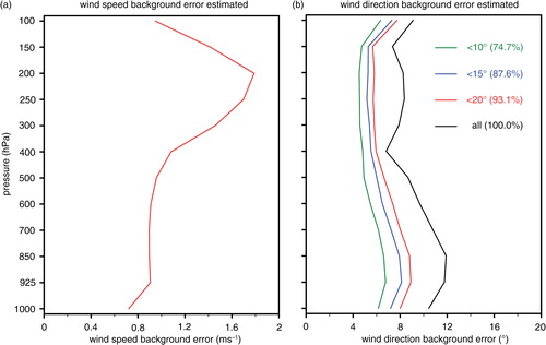
The default spd observation error in WRFDA is also used as the observation errors of u and v in asm_uv, and is employed as the spd observation error (σ _spd ) for asm_sd in this study. The statistics of dir background error can be impacted from situations where grid points with background errors deviate greatly from the general range of the dir background error. To eliminate these unstable values, we set a series of maxima below which the dir background error on a grid point will be used in the calculation of the average dir background error. The resulting options for three similar profile patterns of dir background error are presented in Fig. 3b. By setting the maximum to 20°, dir background errors decrease notably at every pressure level, yet 93% of grid points are still used in the statistics. Therefore, dir observation errors are estimated by using the vertical profile of dir background errors with a maximum of 20° (red line).

In Fig. 3, the background errors of spd and dir vary with height, an effect also discussed for observation errors in Gao et al. (2012). Generally, spd (background and observation) error increases with height, and the opposite is true for dir. However, this pattern is not uniformly true, as shown by the profile of dir observational errors indicated in Fig. 4. Note that the spd and dir observation errors estimated here are not intended to maintain consistency with sensor errors, or to agree with the statistics in WRFDA, but to get similar assimilation weights in asm_uv and asm_sd between u and v errors and spd and dir errors. For surface observations, constant spd and dir observation errors are used despite the fact that instrumentation may be placed at slightly different heights.

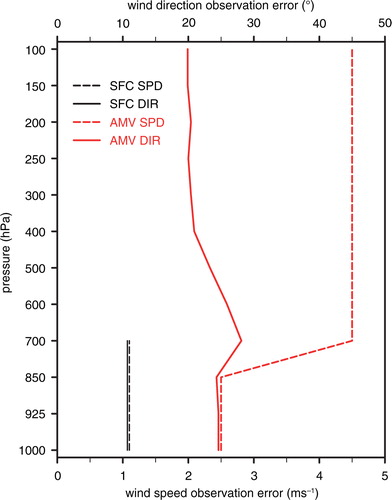
Fig. 4 The observation errors of wind speed (SPD) and direction (DIR) estimated by eq. (3) for MADIS surface wind (SFC) and satellite-derived Atmospheric Motion Vectors (AMV) observations.

3.3. The experiment design

The differences of analyses produced by asm_uv and asm_sd result from the impacts of differences in BKG-QC and the assimilation method itself. To evaluate the performance of asm_sd in these aspects, four assimilation experiments are designed as follows:

1. EX_uv is considered the control run, conventionally employing asm_uv by using the default observation errors defined in WRFDA;

2. EX_sd employs asm_sd by using the estimated observation errors of spd and dir in Fig. 4;

3. EX_sd_uvobs employs asm_sd as EX_sd, but assimilates the same observations used in EX_uv per cycle;

4. EX_sd_sfc employs asm_sd and asm_uv for assimilating surface wind and AMV, respectively.

Since any other observation variable except wind employs the same assimilation scheme among these four experiments, we assume that the differences of wind analyses between EX_uv and EX_sd are derived from the new assimilation method, although it partly includes the impact from the different background at every cycle assimilation. By comparing EX_uv with EX_sd_uvobs, the contribution of the assimilation method itself can be verified due to the same observations used. Thereafter, the impact of BKG-QC can be estimated linearly by subtracting the improvements produced by EX_sd_uvobs from those produced by EX_sd, over EX_uv. Likewise, the exclusive impact of asm_sd on the assimilation of surface wind or AMV observations can be tested by comparing EX_uv with EX_sd_sfc or EX_sd with EX_sd_sfc, respectively.

4. Results

4.1. Distribution of observation by residuals of observation from background and analysis

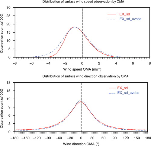
The usage and weight of the observations in the analysis can be demonstrated by the statistical residuals of observation minus background (OMB) and observation minus analysis (OMA). The distributions of surface dir and spd observations by the residuals of OMB and OMA in EX_uv and EX_sd are presented in Fig. 5. From Fig. 5a, a large number of dir observations with innovations (i.e. OMB) exceeding 90°, about 15.0% of all surface dir observations, are assimilated in EX_uv. It appears that BKG-QC in asm_uv does not have a particularly stringent impact on the retention of dir observations.

Fig. 5 The distribution of surface wind direction (a–b) and speed (c–d) observations by observation minus background (OMB, black lines) and observation minus analysis (OMA, red lines) in EX_uv and EX_sd. σ and µ in panels denote the standard deviation and bias of OMB and OMA, respectively.

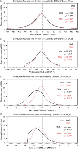
By comparison, dir observations with innovations larger than 90° are screened out directly by BKG-QC in EX_sd (Fig. 5b), which significantly reduces the standard deviation (σ) and bias (µ) of OMB and OMA. It is also worth mentioning that for dir, OMA is even larger than OMB in EX_uv (Fig. 5a), denoting that cost function minimisation in asm_uv does not necessarily converge for dir.

With respect to spd, OMB is biased with the minimum value of −7.1 ms⁻¹ and maximum of 5.4 ms⁻¹ in EX_uv (Fig. 5c). Compared with a sharp cutoff of OMB at −3.3 ms⁻¹ in EX_sd (Fig. 5d), where the BKG-QC directly screens out spd observations meeting eq. (2), BKG-QC of u and v in EX_uv are not able to effectively reject spd observations with large spd OMB, representing a source of strong bias.

As discussed earlier, when dir observations with innovation exceeding 90° are assimilated in asm_uv, spd analysis may be reduced because of the vector nature of u and v. The negative bias in surface spd OMB means that the magnitudes of most spd observations are smaller than the background. Therefore, the spd analysis produced by asm_uv is a closer fit to surface spd observations than the spd analysis produced by asm_sd. As a result, a Gaussian-like pattern of OMA with a relatively small bias (−0.11 ms⁻¹) is seen in EX_uv (Fig. 5c).

By comparison, the bias of surface spd OMA in EX_sd is located between the bias of surface spd OMB and zero (Fig. 5d), demonstrating that the surface spd analysis is reasonably distributed between the observations and background. Due to the fact that surface spd observations are biased in this study, it is acceptable to assume that the spd analysis will over-fit the observations if a near-zero bias exists in OMA. In reality, the uncorrected bias in surface spd observations can be used to prove that the assimilation of biased spd observations is not the primary reason for the large bias of the spd analysis in EX_uv.

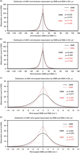
The distribution of AMV dir and spd observations by the residuals of OMB and OMA in EX_uv and EX_sd are shown in Fig. 6. The AMV observations reveal a good fit to the background, such that the BKG-QC in EX_uv and EX_sd only account for a 0.37% difference in observation counts. Although AMV dir OMB mainly appear inside the bounds of ±60° (Fig. 6a and b), the dir observations located in different quadrants from the background still represent approximately 8.0% of all dir observations in EX_uv, and these can be expected to generate some significant impacts on spd analysis in EX_uv.

Fig. 6 The distributions of satellite-derived Atmospheric Motion Vectors (AMV) wind direction (a–b) and speed (c–d) observations by observation minus background (OMB, black lines) and observation minus analysis (OMA, red lines) in EX_uv and EX_sd. σ and µ in panels denote the standard deviation and bias of OMB and OMA, respectively.

4.2. Verification of analysis

The statistical verification presented below is the difference of the analyses and forecasts from RAOB in the form of root-mean-square (rms) and average (bias). Considering the launch time of rawinsondes, the verification is only performed at 0000 and 1200 UTC each day.

The rms difference/error (hereafter referred to as rmse) and bias of spd and dir analyses fit to RAOB in EX_uv and EX_sd is presented in Fig. 7. In Fig. 7a and c, the RAOB data available on the two lowest height levels are used as a reference to present the verification of near-surface wind analysis, where the statistical differences between EX_uv and EX_sd are assumed to be derived from the impact of asm_sd on surface wind data assimilation. Likewise, in Fig. 7b and d, the RAOB data available above the two lowest height levels are used as a reference for verification of upper-air wind analysis, where the statistical differences between EX_uv and EX_sd are assumed to originate from the impact of asm_sd on AMV data assimilation.

Fig. 7 The time series of rmse and bias of wind speed (a–b) and direction (c–d) analyses in EX_uv and EX_sd fit to rawinsonde observations (RAOB). Near-surface RAOB (nlev ≤ 2) denotes RAOB available on two lowest height levels; upper-air RAOB (nlev > 2) denotes RAOB available above two lowest height levels. Black and red lines are statistics in EX_uv and EX_sd; solid and dot lines represent rmse and bias, respectively.

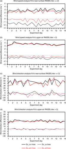
Based on rmse, both spd and dir analyses from EX_sd come closer to RAOB than EX_uv, and the improvement from EX_sd is notable for upper-air locations (Fig. 7b and d) on 1200 UTC 2 August, when the associated precipitation event is examined in Section 4.4. Additionally, the biases of the spd analyses in EX_sd dramatically decrease by 77.5% and 53.0% for near-surface and upper-air locations, respectively (Fig. 7a and b).

Compared with EX_sd, the bias of the spd analysis in EX_uv presents as an inherent discrepancy (cf. Fig. 7a and b), and is likely related to the assimilation method of u and v. As stated above, the BKG-QC only makes a difference of 0.37% in AMV observation counts between EX_uv and EX_sd; therefore, the bias of the spd analysis for upper-air (Fig. 7b) is mainly a function of the assimilation methodology of u and v. In other words, the larger improvements in bias from EX_sd for the near-surface spd analysis also include the impacts of BKG-QC. The BKG-QC results in surface dir observations with innovations exceeding 90°, which account for 15% of all surface dir observation assimilated in EX_uv, but are rejected in EX_sd (cf. Fig. 6a with b). These dir observations also produce an inherent impact on the spd analysis in addition to spd observations in asm_uv.

4.3. Impacts of BKG-QC and assimilation methods on analysis

The improvements from asm_sd are produced jointly from the new method and BKG-QC. The time series of rmse and bias of spd and dir analyses in EX_uv and EX_sd_uvobs is presented in Fig. 8.

Fig. 8 The time series of rmse and bias of wind speed (a) and direction (b) analyses in EX_uv and EX_sd_uvobs fit to rawinsonde observations (RAOB). Black and red lines are the statistics in EX_uv and EX_sd_uvobs; solid and dot lines represent rmse and bias, respectively.

The BKG-QC difference between asm_uv and asm_sd may be ignored in the two experiments due to fact that the same observations have been assimilated. Thus, the new assimilation method is assumed to produce the analysis differences between EX_uv and EX_sd_uvobs. As a result, the impact of BKG-QC can be estimated linearly by subtracting improvements produced by EX_sd_uvobs from the improvements produced by EX_sd compared to EX_uv. The improvements of dir analysis, shown by the rmse decreasing from 6.9% in EX_sd to 5.0% in EX_sd_uvobs, suggest that the new assimilation method produces a more positive impact on the dir analyses than BKG-QC, which only contributes 1.9%.

In terms of spd, BKG-QC in asm_sd plays an important role in improving the rmse of spd analyses by effectively screening out biased spd observations (Fig. 5d). However, the spd bias is largely unchanged with improvements of 54.8% in EX_sd and 54.4% in EX_sd_uvobs. This result demonstrates that the improvement on spd bias is mainly derived from the new assimilation method, i.e. the independent impact of spd (dir) observations on the spd (dir) analysis. This conclusion is also supported by Fig. 9, which shows the spd OMA for EX_sd and EX_sd_uvobs, as well as the dir OMA for EX_uv and EX_sd_uvobs.

Fig. 9 The distribution of surface wind speed observations by observation minus analysis (OMA) in EX_sd and EX_sd_uvobs (a) and of surface wind direction observations by observation minus analysis (OMA) in EX_uv and EX_sd_uvobs (b).

Compared with EX_uv, the cost function related to dir converges in EX_sd_uvobs; therefore, the standard deviation of dir OMA in EX_sd_uvobs is smaller than that in EX_uv (Fig. 9b). However, as seen in Fig. 9a, unlike in EX_uv (Fig. 5c), the assimilation of dir observations with large innovations (e.g. >90°) in EX_sd_uvobs does not prompt spd analyses to over-fit to spd observations. The main differences of spd OMA between EX_sd_uvobs and EX_sd have ranges of −6 ms⁻¹ and −2 ms⁻¹, and these are actually derived from the assimilation of more spd observations with large negative OMB, which are rejected in EX_sd but used in EX_uv (Fig. 5c and d).

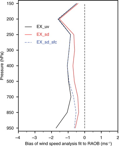
As stated above, the improvement on the bias of spd analyses is the primary feature of asm_sd. As such, a qualitatively consistent conclusion should also exist when employing asm_sd for the assimilation of either surface wind or AMV observations. The bias profile of spd analyses in EX_uv, EX_sd, and EX_sd_sfc is shown in Fig. 10. Below 700 hPa, the significant positive impact produced by asm_sd on surface spd data assimilation can be seen by comparing EX_uv and EX_sd_sfc. Compared to upper-air locations, more improvements are generated on surface spd analyses because BKG-QC in asm_sd plays a more important role in screening out surface dir observations with large dir innovations than AMV dir observations. In terms of AMV, although there is a good fit to the background (Fig. 6a), the dir observations that have different quadrants from the background still generate a notable impact on the bias of the spd analysis. This result strongly supports the importance of the independent impact of the wind observation variables on the wind analysis.

Fig. 10 The biases of wind speed analyses in EX_uv, EX_sd and EX_sd_sfc fit to rawinsonde observations (RAOB).

4.4. Verification of forecast

4.4.1. The statistical characteristics.

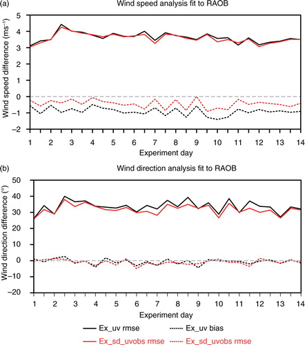
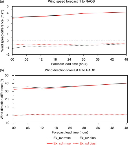
The rmse and bias of spd and dir forecasts of all cycles by forecast lead time are presented in Fig. 11. The forecast improvements from asm_sd are mainly reflected in the bias of spd and rmse of dir, and are consistent with the conclusions for the analyses. Although the forecast differences decrease with lead time because the same lateral boundary conditions are employed for the comparative experiments, the bias of spd forecast in EX_sd are still present at 48 h.

Fig. 11 The rmse and bias of wind speed and direction forecasts in EX_uv, EX_sd fit to rawinsonde observations (RAOB) by forecast lead time.

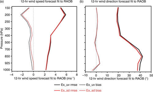
From the vertical profiles of 12-h forecast scoring (Fig. 12), dir forecast rmse in EX_sd is improved over EX_uv at all height levels, and the biases around 1000 hPa and 500 hPa in EX_sd are only little larger than EX_uv. The significant improvements on biases of the spd forecast in EX_sd can still be seen at all height levels; however, the near-surface improvements are reduced by the restriction of the lateral boundary condition (cf. Fig. 7a). The improvement in the rmse of spd forecasts in EX_sd are especially appreciable in light of the non-optimal configuration and tuning in EX_sd. Similar forecast scoring is seen for asm_sd without the negative impacts on spd forecasts, such as those near 400 hPa (Fig. 12a).

Fig. 12 The vertical profiles of rmse and bias of 12-h wind speed and direction forecasts in EX_uv and EX_sd fit to rawinsonde observations (RAOB).

4.4.2. A case for illustration.

In this section, we explore how the improved wind analysis and forecast affect precipitation prediction. In WRFDA, the background error covariance does not include the covariances between moisture and other state variables. Therefore, the different moisture analyses between asm_uv and asm_sd are derived from the cycling assimilation, where the wind forecast adjusts the distribution of moisture, and then the updated moisture forecast is accumulated into the subsequent timestep's background and analysis.

At 1200 UTC 2 August 2013, a stream of warm moist air flowed towards the Kansas/Missouri (KS/MO) border where a cold dry air mass was in place. A frontal shear line developed over northern Illinois (IL) and Indiana (IN) along the boundary between the two air masses. The 24-h accumulated precipitation was heaviest (116 mm) near KSGF station in Springfield, MO (black dot in Fig. 14a).

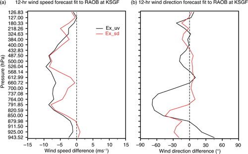
The vertical profiles of 12-h spd and dir forecasts valid at 1200 UTC 3 August 2013 fit to RAOB at KSGF station are shown in Fig. 13. Generally, the spd and dir predictions are improved in EX_sd mainly below 400 hPa. From Fig. 13a, both EX_uv and EX_sd under predicted spd. As a result, the warm moist air advection was reduced in the model. The negative difference between the dir forecast in EX_sd and RAOB below 700 hPa indicates that the predicted dir points to the north-northwest of the observed wind vector, which leads to a more westerly-tilting weather system with respect to observations. Compared to EX_sd, the spd and dir forecasts from EX_uv further exacerbate these problems.

Fig. 13 The differences of 12-h wind speed and direction forecasts valid at 0000 UTC 3 August 2013 in EX_uv and EX_sd from rawinsonde observations (RAOB) at KSGF station in Springfield, Missouri.

A plot of precipitation, wind vectors, and specific humidity in the mixed layer is shown in Fig. 14. Three main differences in the prediction of precipitation location and intensity between EX_sd and EX_uv can be seen along the border of KS and MO, the northern portions of IL and IN, and in southern South Dakota (SD). As discussed for Fig. 13, the weaker warm moist air advection in EX_sd reduces the precipitation intensity along the border of KS and MO in EX_sd. Meanwhile, the northwest-tilting dir, and the corresponding specific humidity gradient, lead to a prediction of the main precipitation area being located northwest of the observed precipitation maximum from the Stage IV analysis near KSGF (Fig. 14c). As expected, the further westerly-tilting dir forecast in EX_uv fails to properly develop the primary precipitation zone in central KS (Fig. 14b).

Fig. 14 The Stage IV 24-h accumulated precipitation analysis (shaded) valid at 1200 UTC 3 August 2013 in (a); the analyses of wind (vector) at 850 hPa and specific humidity (red line) at 700 hPa at 1200 UTC 2 August 2013 and 24-h accumulated precipitation forecasts (shaded) valid at 1200 UTC 3 August 2013 in EX_uv (b) and EX_sd (c). The unit for precipitation is mm, for specific humidity is g kg⁻¹, and for wind vector is ms⁻¹. The black dot in (a) denotes the rawinsonde station KSGF in Springfield, Missouri. South Dakota, Kansas, Missouri, Illinois and Indiana are abbreviated to SD, KS, MO, IL and IN, respectively.

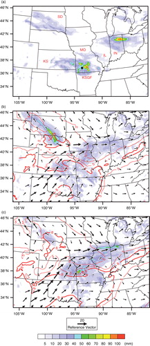
Another key difference can be seen in southern SD, where weak winds exist in EX_sd (Fig. 14c). However, the stronger wind shear, coinciding with a moisture maxima, produces the main precipitation core over southern SD in EX_uv (Fig. 14b). These results demonstrate that the improved wind forecast is able to improve the precipitation forecast by adjusting the wind-related factors driving the intensity and location of precipitation development via moisture advection.

5. Conclusion and outlook for further research

This paper presents a series of real-data experiments to evaluate the assimilation of wind observations in the forms of wind speed (spd) and direction (dir). The potential benefits of this method were verified over a continental United States domain for a 2-week period in the cycling assimilation. Satellite-derived Atmospheric Motion Vectors (AMV) and surface data from Meteorological Assimilation Data Ingest System (MADIS) were assimilated, and their spd and dir observation errors were estimated for the purpose of assigning similar assimilation weights for wind observations in asm_uv and asm_sd. Using rawinsonde observations (RAOB) and National Centers for Environmental Prediction (NCEP) Stage IV analysis as references, the statistical verification of the wind analyses, forecasts and a precipitation case study are presented.

Results demonstrate that the asm_sd produces better analyses and forecasts compared to asm_uv based on rmse and bias. Improvement up to 54.8% is generated by asm_sd for the bias of spd analyses, and persists through the 48-h forecasts despite using identical lateral boundary conditions. In a pilot test (EX_sd_uvobs) employing asm_sd, but assimilating the same observations as EX_uv, we show that the significant improvement in bias of spd analysis was primarily from the new assimilation method.

The background quality control (BKG-QC) in WRFDA is also a key factor in improvements of asm_sd over asm_uv. In the total rmse improvement of 3.7% for spd analyses and 6.9% for dir analyses, the 2.3% and 1.9% for spd and dir analyses are derived solely from the BKG-QC of asm_sd, respectively. Generally speaking, some benefits from asm_sd were produced from BKG-QC screening wind observations, but most benefits originated from the new assimilation method itself.

The indirect impacts of asm_sd on precipitation prediction were examined using an event which occurred during the experimental period. Results suggest that the asm_sd is able to improve the forecast of precipitation intensity and location by improving the prediction of wind-related dynamics.

Given the limitations of the experimental design, some differences may exist with operational applications. The observational errors are not optimally tuned when it comes to the assimilation weights between observations and background. The equivalent wind observation errors estimated and presented here for asm_uv and asm_sd are more focused on making a fair comparison of the assimilation scheme.

The BKG-QC in asm_sd needs to be further studied. It is likely that the innovation threshold of 90° for dir observations is too strict to retain most useful observations. For example, in the precipitation case presented, some good dir observations with an innovation score above 90° were observed in the vicinity of the frontal system when a phase difference exists between the observations and the background. Further investigations of the estimation and tuning of spd and dir observation errors for all wind observation types and the corresponding BKG-QC scheme should be conducted.

Additionally, although the mass variables in the surface dataset are also assimilated along with the wind observations, the proportion of wind-to-mass observations in this study is skewed towards the impact of wind observations versus what would be expected in an operational configuration.

Another interesting topic exists regarding BKG-QC of wind observations in asm_uv that deserves investigation. As discussed, the BKG-QC in asm_uv is conducted for the u and v components separately, which means that either u or v could be rejected or assimilated without the other. However, it seems unreasonable to assimilate the other variable when its respective component is rejected because the u and v components are calculated from a single observational pair of spd and dir, and the observation error in either spd or dir can simultaneously affect the errors in both u and v. Is alone u or v able to usefully contribute to wind vector analyses when one of them is rejected? Or is it more helpful to reject both of them when one of them fails QC? The question is not addressed here, but is worthy of further discussion.

6. Acknowledgements

The authors thank Jun-Mei Ban (NCAR) for the converting code of NCEP Stage IV precipitation analysis. We are also grateful for the invaluable comments and suggestions from three anonymous reviewers. The first author acknowledges the support of National Natural Science Foundation (41430427), 973 program (2013CB430102) and Panasonic Avionics Corporation.

Notes

¹ www.nws.noaa.gov/asos/pdfs/aum-toc.pdf

²Horizontal speed in which the aircraft moves relative to a fixed point on the ground.

³Speed in which the aircraft moves relative to the surrounding air.

⁴ rammb.cira.colostate.edu/projects/goes-p/NOAA_Technical_Report_141_GOES-15_Science_Test.pdf

⁵ www.star.nesdis.noaa.gov/star/documents/seminardocs/EUMet_Products.pdf

⁶ madis.noaa.gov

References

- Andersson E. , Haseler J. , Undén P. , Courtier P. , Kelly G . The ECMWF implementation of three-dimensional variational assimilation (3D-Var). III: experimental results. Q. J. Roy. Meteorol. Soc. 1998; 124: 1831–1860.
- Barker D. , Huang X.-Y. , Liu Z. , Auligné T. , Zhang X . The weather research and forecasting (WRF) model's community variational/ensemble data assimilation system: WRFDA. Bull. Am. Meteorol. Soc. 2012; 93: 831–843.
- Benjamin S. G. , Schwartz B. E. , Cole R. E . Accuracy of ACARS wind and temperature observations determined by collocation. Weather Forecast. 1999; 14: 1032–1038.
- Drüe C. , Frey W. , Hoff A. , Hauf T . Aircraft type-specific errors in AMDAR weather reports from commercial aircraft. Q. J. Roy. Meteorol. Soc. 2008; 134: 229–239.
- Gao F. , Zhang X. Y. , Jacobs N. A. , Huang X.-Y. , Zhang X . Estimation of TAMDAR observational error and assimilation experiments. Weather Forecast. 2012; 27: 856–877.
- Gustafsson N. , Berre L. , Hornquist S. , Huang X.-Y. , Lindskog M . Three-dimensional variational data assimilation for a limited area model. Tellus A. 2001; 53: 425–446.
- Hollingsworth A. , Lönnberg P . The statistical structure of short-range forecast errors as determined from radiosonde data. Part I: the wind field. Tellus A. 1986; 38A: 111–136.
- Huang X-Y. , Gao F. , Jacobs N. A. , Wang H . Assimilation of wind speed and direction observations: a new formulation and results from idealized experiments. Tellus A. 2013; 65 19936.
- Huang X.-Y. , Xiao Q. , Barker D. , Zhang X. , Michalakes J . Four-dimensional variational data assimilation for WRF: formulation and preliminary results. Mon. Weather Rev. 2009; 137: 299–314.
- Jarvinen H. , Andersson E. , Bouttier F . Variational assimilation of time sequences of surface observations with serially correlated errors. Tellus A. 1999; 51: 469–488.
- Kalnay E. , Kanamitsu M. , Kistler R. , Collins W. , Deaven D . The NCEP/NCAR 40-year reanalysis project. Bull. Am. Meteorol. Soc. 1996; 77: 437–471.
- Le Dimet F. , Talagrand O . Variational algorithms for analysis and assimilation of meteorological observations: theoretical aspects. Tellus A. 1986; 38A: 97–110.
- Lin Y. , Mitchell K. E . The NCEP stage II/IV hourly precipitation analyses: development and applications. Preprints, In: . 19th Conference on Hydrology. 2005; San Diego, CA: American Meteorological Society.
- Lindskog M. , Gustafsson N. , Navascués B. , Mogensen K. S. , Huang X.-Y . Three-dimensional variational data assimilation for a limited area model. Part II: Observation handling and assimilation experiments. Tellus A. 2001; 53A: 447–468.
- Moninger W. R. , Benjamin S. G. , Jamison B. D. , Schlatter T. W. , Smith T. L. , co-authors . Evaluation of regional aircraft observations using TAMDAR. Weather Forecast. 2010; 25: 627–645.
- Painting D. J . AMDAR reference manual. 2003. WMO, 84 pp. Online at: http://amdar.wmo.int/Publications/AMDAR_Reference_Manual_2003.pdf .
- Parrish D. F. , Derber J. C . The National Meteorological Center's Spectral Statistical Interpolation analysis system. Mon. Weather Rev. 1992; 120: 1747–1763.
- Plant W. J . Effects of wind variability on scatterometry at low wind speeds. J. Geophys. Res. 2000; 105: 16899–16910.
- Skamarock W. , Klemp J. , Dudhia J. , Gill D. , Barker D . A Description of the Advanced Research WRF Version 3. 2008. NCAR Tech. Note, 2008. NCAR/TN–475 + STR. pp. 1–113.
- Velden C. S. , Olander T. L. , Wanzong S . The impact of multispectral GOES-8 wind information on Atlantic tropical cyclone track forecasts in 1995. Part I: Dataset methodology, description, and case analysis. Mon. Weather Rev. 1998; 126: 1202–1218.
- Wu W. S. , Purser R. J. , Parrish D. F . Three-dimensional variational analysis with spatially inhomogeneous covariances. Mon. Weather Rev. 2002; 130: 2905–2916.