Note on the redistribution and dissipation of tidal energy over mid-ocean ridges

Abstract

The redistribution and dissipation of internal wave energy arising from the conversion at mid-ocean ridges of the barotropic tide is studied in a set of numerical experiments. A two-dimensional non-hydrostatic model with 100 m horizontal and 10–25 m vertical resolution is used to represent the detailed processes near an idealised ridge. Conventional internal wave beams at the tidal frequency, ${\omega }_{M_2}$, appear. At the ridge crest, strong tidal energy dissipation occurs that both mixes the fluid and generates strong near-inertial oscillations radiating in near-horizontal beams. Resonant triad interaction between the tidal and inertial motions in turn produces beams at $\left({\omega }_{M_2}-f\right),$ and with high shear, thus effectively mixing fluid at considerable heights above the ridge crest.

• tides
• internal waves
• energy dissipation
• resonant triad interaction

1. Introduction

Internal waves remain the main candidate for the mechanism by which the ocean is mixed (e.g. Thorpe, 1975). Recently, much attention has been focussed on the internal tide as the central element in generating an internal wave field capable of providing the requisite power and shears needed (e.g. Garrett and Kunze, 2007). Numerous recent studies include Khatiwala (2003); Legg and Klymak (2008) and Nikurashin and Legg (2011). The latter (hereafter NL11) provided an interesting and useful discussion of the two-dimensional problem, suggesting that the non-linear wave–wave (resonant triad) interactions are the dominant mechanism by which mixing is ultimately controlled.

The purpose of this present note is to better understand, in a somewhat simpler, even more idealised, configuration than the one used by NL11, the mechanisms by which non-linear interactions are generated in a two-dimensional stratified rotating ocean with topography. It is intended to elucidate the evolution and fate of baroclinic motions induced by scattering of a barotropic motion over a simple topographic obstruction. The NL11 configuration involved a complex, broad-band, random one-dimensional topography as represented in the MITgcm (Marshall et al., 1997). They showed that the model, when forced by a depth-independent horizontal flow of frequency $\omega ={\omega }_{M_2}$, could generate a powerful baroclinic tidal peak, a weaker inertial motion (frequency ω=f) and the basic tidal overtones (integer multiples $\omega =n{\omega }_{M_2}$), as well as the fundamental interaction frequencies $\omega ={\omega }_{M_2}\pm f$. Even more remarkably, although little is made of it, their configuration produced a continuum kinetic energy frequency spectrum f≤ω≤N, where N is the buoyancy frequency, indistinguishable in shape from that of Garrett and Munk (e.g. Garrett and Munk, 1972, see Fig. 9 in NL11). Assuming the modelled motions do indeed represent internal waves and not numerical noise, their result may be the first time that a GCM has reproduced a full, realistic internal wave continuum. Although the subject is not pursued here, the result can be interpreted to imply that the oceanic internal wave field can be sustained by tidal input alone, not requiring any other energy source (see e.g. Thorpe, 1975).

NL11 concluded that the radiated internal tides, despite being energetic, are stable to shear instability. Thus a major portion of the observed intense mixing within O(1) km above rough topography (e.g. Polzin et al., 1997) would be sustained by the energy transferred from the propagating internal tides through a resonant triad interaction formed among motions at ${\omega }_{M_2}$, ${\omega }_{M_2}\pm f$ and f. Because of the complicated topography and the superposition of a variety of beams, NL11 did not explicitly show the locations where the resonant triad interaction occurs. Locating these regions would provide useful information about the formation of the resonant triad interaction and serve as a reference for designing in situ observations to confirm those dynamical processes. With a simpler bathymetry, it is possible to isolate the regions of occurrence of the resonant triad interactions, and their initialisation.

2. Model configuration

Consider a two-dimensional model ocean with a simple ridge. As in NL11, the MITgcm (Marshall et al., 1997) is used in non-hydrostatic form. The horizontal domain spans 120 km. Bathymetry is centred in the domain as1 $H=H_{deep}-H_{relief}{e}^{-(\mid x-x_0\mid )/\delta },$1

where x is distance in the east–west direction, x ₀=60 km is the location of the ridge crest, H _deep =3200 m, H _relief =700 m, and δ=6 km. The prototype of the topography is the East Pacific Rise (EPR). The topographic shape and the related parameters in eq. (1) were estimated by fitting ridge-normal transects of bathymetric data of a segment of the EPR (e.g. Lavelle, 2012). McGillicuddy et al. (2010) also used the same topography to represent the EPR in a biological study. Horizontal grid spacing is 100 m, with a vertical grid varying with depth, from 10 m at the bottom of the ridge, and increasing to 25 m near the surface. Note that this topography is ‘subcritical’ for the M ₂ tide beam everywhere, and it is different from the commonly utilised ridge configuration that has ‘supercritical’ slope and a rounded top (e.g. Khatiwala, 2003; Legg and Klymak, 2008).

Lateral boundary conditions are periodic; the bottom is no-slip. To eliminate interactions between the upward-propagating and possible reflected downward-propagating beams and to minimise the influence of the periodic lateral boundaries, a 2.5-km thick sponge layer is added 3200 m above the sea-floor to absorb the upward-propagating tidal energy. In the sponge layer, both buoyancy and momentum are damped with a linear drag on a time scale of 1 hour.

Stratification is constant (N=10⁻³ s⁻¹, period 1.8 hour) with the Coriolis frequency (f=0.53′ 10⁻⁴ s⁻⁴, period 33 hours) corresponding to a latitude far from the so-called critical latitude of semidiurnal tides where the specific resonant triad interaction called the ‘parametric subharmonic instability’, or PSI, becomes potentially important (e.g. MacKinnon and Winters, 2005). Horizontal (ν _h ) and vertical viscosity (ν _r ) are both set to 10⁻³ m² s⁻¹ and the horizontal (κ _h ) and vertical diffusivities (κ _r ) are 10⁻⁴ m² s⁻¹. A body force is used to generate a barotropic tide with a frequency of 1.4×10⁻⁴ s⁻¹ (M ₂ tide) and an amplitude of 2.5 cm s⁻¹. Seven harmonics of M ₂ tide are permitted within the prescribed frequency range. In this configuration, the model was run for 100 d with a time step of 2 minutes.

A few other runs with forcing ranging between 1 and 10 cm s⁻¹ show almost identical results (qualitatively) as presented here, except that the amplitudes of the different frequency components increase/decrease with stronger/weaker forcings. As in NL11, the time scale of the non-linear interaction generally decreases with stronger forcing. But, runs with much weaker forcing (i.e. 0.5 cm s⁻¹) show different results, suggesting a dynamical shift with the changing strength of forcing, that is, significant non-linearity.

3. Results

After about 20 d, the model reached a visually steady-state. A snapshot of the zonal velocity on day 80 appears in Fig. 1. Three pairs of internal wave beams, distinguished by their slopes, α, are emitted from the ridge crest. The internal wave dispersion relation produces2 $\alpha =\frac{\sqrt{{\omega }^2-f^2}}{\sqrt{N^2-{\omega }^2}}.$2

Fig. 1 Horizontal velocity on day 80. Beam 1, beam 2 and beam 3 are associated with frequencies ${\omega }_{M_2}$, ${\omega }_{M_2}-f$ and f, respectively. Dots show locations where the zonal velocities are used to estimate the frequency spectra (Fig. 2).

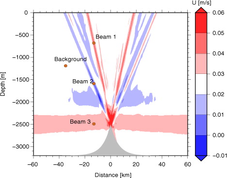
Slopes of the beams marked 1–3 in Fig. 1 correspond to internal waves at frequencies of M ₂, M ₂–f and f, respectively (written as ${\omega }_{M_2},{\omega }_{M_2}-f,$ etc.). Beam 1, for ${\omega }_{M_2}$, can be rationalised by linear internal tide generation theory (e.g. Bell, 1975). However, beams 2 and 3 necessarily arise from one or more non-linear interaction mechanisms. Outside the beams, zonal velocities u, are of similar amplitude and direction and are dominated by the forced barotropic M ₂ tide. Note that both barotropic and baroclinic components contribute to the beams at ${\omega }_{M_2}$. Because the barotropic component is homogeneous in the whole domain, any difference emerging from the background is due to the baroclinic component.

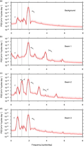
Spectral analyses of u sampled at different points in the domain confirm that the dominant frequencies of the three beams are as labelled (Fig. 2). A variety of non-linear processes occur in the simulation and vary from region to region. For example, the dominant spectral peaks in beam 1 are at ${\omega }_{M_2}$ and its harmonics ($2{\omega }_{M_2}$ and $3{\omega }_{M_2}$). In contrast, no clear spectral peaks at tidal harmonics appear in beams 2 and 3. Beam 2 shows peaks near f, ${\omega }_{M_2}-f$, ${\omega }_{M_2}$ and $2{\omega }_{M_2}-f$. The peak near ${\omega }_{M_2}-f$ would be the result of the interaction of ${\omega }_{M_2}$ and f, and the interaction of ${\omega }_{M_2}-f$ and ${\omega }_{M_2}$ would result in the peak near $2{\omega }_{M_2}-f$. Beam 3 shows a peak near the local inertial frequency, corresponding to a variance of 1.6×10⁻⁴ m² s⁻², about 1000 times larger than outside (≈1.2×10⁻⁷ m² s⁻²). Beam 3 also shows a spectral peak near ${\omega }_{M_2}$, but none near ${\omega }_{M_2}\pm f$. This result suggests that the interaction between ${\omega }_{M_2}$ and f occurs only in specific regions, because otherwise spectral peaks would appear near ${\omega }_{M_2}\pm f$ in beam 3.

Fig. 2 Frequency spectra of the horizontal velocities sampled at different points in the simulated domain. The locations of the sampled points are listed in the right-upper corner of each panel and are marked in Fig. 1. Approximate 95% confidence intervals are marked with thin red curves and the number of degrees-of-freedom is about 10. Three vertical black lines show the theoretical frequencies (from left to right: f, ${\omega }_{M_2}-f$ and ${\omega }_{M_2}$).

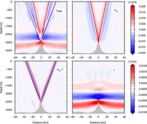
Snapshots of u at different frequencies (total, ${\omega }_{M_2}$, ${\omega }_{M_2}-f$ and f) in the steady-state show that, as expected, the plane waves propagate perpendicular to the beams (Fig. 3). The vertical characteristic scales of the superpositions of those plane waves can be estimated at the different frequencies and Fig. 3 shows u in different bands on day 80. The dominant vertical scales of the plane wave superpositions associated with the beams at ${\omega }_{M_2}$, ${\omega }_{M_2}-f$ and f are about 1000 m, 300 m and 800 m, respectively. The very different values imply differing shear stability. Vertical wavenumber spectra of the snapshots of u in different bands show dominant peaks near (0.4–1.2)×10⁻³ cpm (cycle per meter) and (2.3–3.1)×10⁻³ cpm for f and ${\omega }_{M_2}-f$, respectively. For ${\omega }_{M_2}$, despite the largest peak appearing near 0.4×10⁻³ cpm, the second largest peak is near (1.9–2.7)×10⁻³ cpm, which can form a triad with the dominant wavenumber components at f and ${\omega }_{M_2}-f$.

Fig. 3 Zonal velocities in different frequency bands on day 80. (a) The total frequency bands, (b) ${\omega }_{M_2}$, (c) ${\omega }_{M_2}-f$ and (d) f. Frequency bands are listed in the right-upper corner of each panel. Note the phase change of the zonal velocities near the beams.

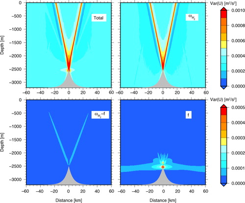
The four panels in Fig. 4 show the variances of the zonal velocities in the whole frequency band, and of the three dominant beams. Those at ${\omega }_{M_2}$ are energetically dominant. Kinetic energy generation occurs at and near the ridge crest, with the strongest flows at all frequency components appearing in a limited region there.

Fig. 4 Variances of zonal velocities in different frequency bands after the model reaches a steady-state. (a) The total in all frequency bands, (b) ${\omega }_{M_2}$, (c) ${\omega }_{M_2}-f$ and (d) f. In the upper two panels, the values outside of the beams are mainly due to the barotropic M ₂ tides. Note the different colour limits for the upper and lower panels.

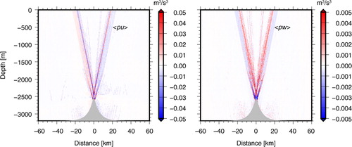
As in Nash et al. (2005), energy flux is a useful diagnostic of energy transfer and can be estimated from the wave-induced velocity (u) and pressure (p). Temporal means of pu and pw are shown in Fig. 5. As in previous studies (e.g. Klymak et al., 2012), the converted tidal energy at the ridge crest mainly propagates away along the M ₂ beams. The energy flux along the M ₂–f beams is smaller than in the M ₂ beams and is barely visible in the temporally averaged horizontal and vertical energy fluxes (<pu> and <pw>). This result indicates that the M ₂–f beams contribute little to the energy transfer away from the ridge crest, even though, as shown later, they are the most dissipative regions in the whole domain, excluding the immediate vicinity of the ridge crest. A weak downward energy flux propagating towards the ridge crest appears below the main beams, consistent with the spatial pattern of the zonal velocity at ${\omega }_{M_2}$ (Fig. 3). With longer averaging time, the downward-propagating energy flux is expected to approach zero.

Fig. 5 Horizontal and vertical energy fluxes. (a) <pu>, (b) <pw>. Here <> represents temporal averaging after the model reaches the steady-state.

Tidal energy propagating away from the ridge crest must dissipate. The turbulent kinetic energy dissipation rate () is estimated as3 $\mathrm{∊}=\nu <{(\frac{\partial u}{\partial z})}^2+{(\frac{\partial v}{\partial z})}^2>$3

where ν=ν _r (10⁻³ m²/s); u and v are the zonal and meridional velocities, respectively; <> represents temporal averaging after the model reaches steady-state and ε is shown in Fig. 6. The strongest dissipation far from the ridge crest appears along two upward-directed beams which, surprisingly, are not the energetic M ₂, but the weaker M ₂–f beams. Moreover, dividing the total energy by the estimated ε provides time scales indicating the relative rate of dissipation. The fastest dissipation also occurs along the M ₂–f beams with decay time scales of about 30 d near the ridge crest and 100 d near the surface. Outside of the M ₂–f beams, decay time scales are all above 200 d. It is intriguing that despite the energy level of the M ₂–f beams being lower than in the M ₂ beams (Fig. 4), they dissipate more energy and more quickly and are thus potential sites of greater mixing above ocean ridges.

Fig. 6 Temporal means of the estimated energy dissipation rates and related quantities. (a) Shear, (b) buoyancy frequency, (c) gradient Richardson number (Ri) and (d) turbulent energy dissipation rate (ɛ).

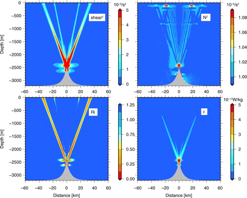
Figure 6 shows the mean Richardson number (Ri) in the steady-state. Two upward-directed beams at ${\omega }_{M_2}-f$ and four near-horizontal beams at f are associated with small Ri (<0.5) and are therefore presumably less stable than is the rest of the fluid (e.g. Turner, 1979). Temporal means show that the small Ri along the M ₂–f and f beams is mainly due to the strong shear; recall Fig. 3.

The temporal evolution of the different frequency components in the early stage of the simulation provides some insights into the generation mechanisms. After initialisation, the beams at ${\omega }_{M_2}$ appear and reach a visually steady-state almost immediately. In contrast, several model-weeks are required for the M ₂–f and f beams to be fully developed. Figure 7 displays the temporal evolution of u in different frequency bands at a point 200 m above the ridge crest. Amplitudes of u at ${\omega }_{M_2}-f$ and f increase simultaneously from zero to visually steady values (${\omega }_{M_2}-f$: 0.12 m/s; f: 0.15 m/s) in about 20 d; at the same time, the amplitude of u at ${\omega }_{M_2}$ decreases from 0.06 m/s to 0.05 m/s, consistent with the extraction of energy from the M ₂ tides. Note other non-linear processes also occur (Fig. 2), so not all the energy lost at ${\omega }_{M_2}$ is transferred into ${\omega }_{M_2}-f$ and f. Temporal evolution of the zonal velocities at ${\omega }_{M_2}-f$ (Fig. 8) indicates that the M ₂–f beams develop initially from the ridge crest, consistent with generation there.

Fig. 7 Temporal evolution of the different frequency components at a point 200 m above the ridge crest. The four panels from top to bottom are zonal velocity in the total frequency bands, ${\omega }_{M_2}$, ${\omega }_{M_2}-f$ and f, respectively. Note the decrease of the amplitude of u at ${\omega }_{M_2}$ and the increase of the amplitudes of u at ${\omega }_{M_2}-f$ and f in the first 20 d.

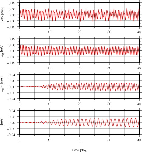
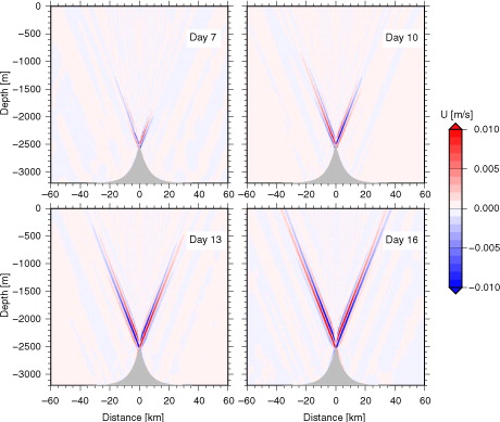
Fig. 8 Temporal evolution of the M ₂–f beams in the early stage of the simulation.

4. Discussion

Three pairs of internal wave beams (${\omega }_{M_2}$, ${\omega }_{M_2}-f$ and f) are formed at the ridge crest in the simulation forced by a barotropic tide at the M ₂ frequency. Although the beams at ${\omega }_{M_2}-f$ and f are not as energetic as at ${\omega }_{M_2}$, they dissipate more energy and are thus the likely regions of strong mixing away from the ridge crest. Relationships among the frequencies and the vertical wavenumbers of the plane waves associated with the three pairs of beams are consistent with their formation from a resonant triad interaction.

As in NL11, the radiated internal tides are stable to shear instability, but resonant triad interactions permit strong dissipation at frequency ${\omega }_{M_2}-f$. A major difference from their conclusions is that here the resonant triad interaction appears important only in a very limited region near the ridge crest (Figs. 2 and 8), rather than in an extended region above the topography. Generation of near-inertial oscillations (NIOs) being limited to near the ridge crest can explain the localisation of the resonant triad interactions in the present results. Because topography is the only major difference between the two studies, the different results suggest that, as in the near-field scattering problem (e.g. Maas, 2011), the redistribution and dissipation of the converted tidal energy are sensitively dependent on the topographic details.

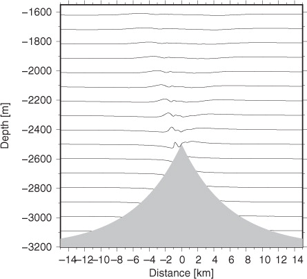
The initialisation of NIOs is key in forming the resonant triads here. NL11 attributed the generation of NIOs to the response of large-scale flows to the breaking of internal tides. In contrast, Korobov and Lamb (2008) proposed that NIOs are the results of PSI. Studies of the gravity waves in the atmosphere show that a well-mixed air patch can generate NIOs through instability processes (Bühler et al., 1999). To evaluate these mechanisms, another simulation was done here using the same model configuration, except that the period of forcing was changed to 5 d – much longer than the imposed local inertial period. The result is again the generation of NIOs near the regions of low Ri, mainly in a limited region over the ridge crest. Furthermore, many internal wave beams at frequencies higher than f are also emitted from the regions of low Ri. When the forcing frequency is below f, PSI is impossible (McComas and Bretherton, 1977), and that mechanism cannot directly explain the appearance of NIOs. The adjustment processes of the mixed fluid, which are related to the breaking of internal M ₂ tides (e.g. St Laurent and Garrett, 2002) or of the arrested lee waves (e.g. Klymak et al., 2008) near the ridge crest, could be the dominant mechanism for the initial generation of NIOs in the present simulations. The existence of lee waves is made evident in the early stage of our simulations before internal tides are fully evolved (Fig. 9). After the resonant triad is formed, NIOs receive further energy directly from the internal M ₂ tides.

Fig. 9 Isothermals at hour 12. A lee wave train appears on the left side of the ridge crest.

A plausible scenario for the redistribution and dissipation of tidal energy over mid-ocean ridges is as follows: when the barotropic tide flows over the ridge crest, internal tides are generated through a primarily linear process. Some elements with high wavenumbers (e.g. St Laurent and Garrett, 2002) and/or in the presence of non-linear processes (e.g. Klymak et al., 2008) occur near the ridge crest, strong energy dissipation results, thus mixing the fluid there. The resulting mixed water patch collapses and generates NIOs, which are the near-horizontal beams appearing in Figs. 1 and 4. Meanwhile, the internal tide and the NIOs with favourable wavenumbers interact to form a resonant triad, which is evident from the relationships among the frequencies (Fig. 2) and dominant wavenumbers (Fig. 3) of the plane waves associated with the distinct beams. As a result, the beams at ${\omega }_{M_2}-f$ are formed and the NIOs are intensified. Furthermore (and similar to the results of PSI), the beams at ${\omega }_{M_2}-f$ and f are composed of components of high vertical wavenumbers and are more unstable. Beams at ${\omega }_{M_2}-f$, rather than at ${\omega }_{M_2}$, can be more important in sustaining the ocean mixing above ocean ridges. In contrast to the inference of NL11, over the mid-ocean ridges non-linear interactions can occur primarily in the vicinity of the ridge crest, but that conclusion is dependent upon topographic details. The topographic shape used in this present study, being ‘subcritical’ for the M ₂ tide beam everywhere, differs from that in many previous studies (e.g. Khatiwala, 2003; Legg and Klymak, 2008), in which topography usually has ‘supercritical’ slopes and a rounded top. In those studies, no lee waves exist and the points with critical slope play an essential role in the tidal energy redistribution and dissipation. In our study, however, no points with critical slope exist, and the lee waves associated with the very short length scale at the crest become crucial.

As with all of the similar published calculations directed at this problem, more elements remain to be considered before the connection between real tidal forcing and mixing could be regarded as well-understood. Among those elements, changes owing to three-dimensionality – in the topography, in the flow field and in the stability properties – loom very large. Note also that β-effects can have a profound influence on the behaviour of near-inertial motions.

Acknowledgements

We thank M. Nikurashin for his help in configuring the model. We are also very grateful to R. Ferrari, O. Bühler and O. Sun for their comments on an early version of this manuscript. Comments from two anonymous reviewers are helpful in improving this manuscript. The work was supported in part by National Science Foundation through Grant OCE-0961713 and National Oceanic and Atmospheric Administration through Grant NA10OAR4310135.

References

- Bell T . Topographically generated internal waves in the open ocean. J. Geophys. Res. 1975; 80: 320–327.
- Bühler O. , McIntyre M. , Scinocca J . On shear-generated gravity waves that reach the mesosphere. Part I: wave generation. J. Atmos. Sci. 1999; 56(21): 3749–3763.
- Garrett C. , Kunze E . Internal tide generation in the deep ocean. Annu. Rev. Fluid Mech. 2007; 39: 57–87.
- Garrett C. , Munk W . Space-time scales of internal waves. Geophys. Astrophys. Fluid Dyn. 1972; 3(1): 225–264.
- Khatiwala S . Generation of internal tides in an ocean of finite depth: analytical and numerical calculations. Deep Sea Res. 2003; 50(1): 3–21.
- Klymak J. M. , Legg S. , Alford M. H. , Buijsman M. , Pinkel R. , co-authors . The direct breaking of internal waves at steep topography. Oceanography. 2012; 25(2): 150–159.
- Klymak J. M. , Pinkel R. , Rainville L . Direct breaking of the internal tide near topography: Kaena Ridge, Hawaii. J. Phys. Oceanogr. 2008; 38(2): 380–399.
- Korobov A. , Lamb K . Interharmonics in internal gravity waves generated by tide-topography interaction. J. Fluid Mech. 2008; 611(1): 61–95.
- Lavelle J . On the dynamics of current jets trapped to the flanks of mid-ocean ridges. J. Geophys. Res. 2012; 117: C07002.
- Legg S. , Klymak J . Internal hydraulic jumps and overturning generated by tidal flow over a tall steep ridge. J. Phys. Oceanogr. 2008; 38(9): 1949–1964.
- Maas L. R . Topographies lacking tidal conversion. J. Fluid Mech. 2011; 684: 5–24.
- MacKinnon J. , Winters K . Subtropical catastrophe: significant loss of low-mode tidal energy at 28.9°. Geophys. Res. Lett. 2005; 32: L15605.
- Marshall J. , Adcroft A. , Hill C. , Perelman L. , Heisey C . A finite-volume, incompressible Navier–Stokes model for studies of the ocean on parallel computers. J. Geophys. Res. 1997; 102: 5753–5766.
- McComas C. , Bretherton F . Resonant interaction of oceanic internal waves. J. Geophys. Res. 1977; 82(9): 1397–1412.
- McGillicuddy D. , Lavelle J. , Thurnherr A. , Kosnyrev V. , Mullineaux L . Larval dispersion along an axially symmetric mid-ocean ridge. Deep Sea Res. 2010; 57: 880–892.
- Nash J. D. , Alford M. H. , Kunze E . Estimating internal wave energy fluxes in the ocean. J. Atmos. Ocean. Technol. 2005; 22(10): 1551–1570.
- Nikurashin M. , Legg S . A mechanism for local dissipation of internal tides generated at rough topography. J. Phys. Oceanogr. 2011; 41(2): 378–395.
- Polzin K. , Toole J. , Ledwell J. , Schmitt R . Spatial variability of turbulent mixing in the abyssal ocean. Science. 1997; 276(5309): 93–96.
- St Laurent L. , Garrett C . The role of internal tides in mixing the deep ocean. J. Phys. Oceanogr. 2002; 32(10): 2882–2899.
- Thorpe S . The excitation, dissipation, and interaction of internal waves in the deep ocean. J. Geophys. Res. 1975; 80(3): 328–338.
- Turner J . Buoyancy Effects in Fluids. 1979; Cambridge, UK: Cambridge University Press.