The impact of waves and sea spray on modelling storm track and development

Abstract

In high wind speed conditions, sea spray generated by intensely breaking waves greatly influences the wind stress and heat fluxes. Measurements indicate that the drag coefficient decreases at high wind speeds. The sea spray generation function (SSGF), an important term of wind stress parameterisation at high wind speeds, is usually treated as a function of wind speed/friction velocity. In this study, we introduce a wave-state-dependent SSGF and wave-age-dependent Charnock number into a high wind speed–wind stress parameterisation. The newly proposed wind stress parameterisation and sea spray heat flux parameterisation were applied to an atmosphere–wave coupled model to study the mid-latitude storm development of six storm cases. Compared with measurements from the FINO1 platform in the North Sea, the new wind stress parameterisation can reduce wind speed simulation errors in the high wind speed range. Considering only sea spray impact on wind stress (and not on heat fluxes) will intensify the storms (in terms of minimum sea level pressure and maximum wind speed), but has little effect on the storm tracks. Considering the impact of sea spray on heat fluxes only (not on wind stress) can improve the model performance regarding air temperature, but it has little effect on the storm intensity and storm track performance. If the impact of sea spray on both the wind stress and heat fluxes is taken into account, the model performs best in all experiments for minimum sea level pressure, maximum wind speed and air temperature.

• sea spray
• wind stress
• heat fluxes
• storms

1. Introduction

Severe storm systems threaten offshore activities as well as coastal and inland areas. Appropriate descriptions of processes such as air–sea interaction can play a role in better forecasts and better climate descriptions of these systems. Air–sea interaction processes are responsible for transporting energy, heat and matter between the ocean and the atmosphere. Momentum and heat fluxes are essential factors affecting storm intensity, storm tracks and precipitation. Appropriate momentum and heat flux parameterisations in numerical models can play an essential role in weather forecasting and climate studies. Although momentum and heat flux parameterisations have been studied for decades, there is no general agreement on their formulation, especially in extreme wind conditions (e.g. Takagaki et al., 2012). Although several wind stress parameterisations exist for high wind speed conditions, their scatter is significant due to the few field data available and uncertainties in the description of sea spray in the wind–sea.

Bulk formulation is the main method used to calculate the momentum flux/wind stress in numerical models. The drag coefficient, C _d , is chosen to build the relationship between wind speed and wind stress, τ, that is, $\tau ={\rho }_a{C}_d{U}_{10}^2$, where ρ _a is the air density and U ₁₀ the wind speed at 10m above mean sea level. Under neutral stratification conditions, the drag coefficient is usually given by1 $C_{dN}={\left(\frac{\kappa }{ln(10/z_0)}\right)}^2$1

where z ₀ is the sea roughness length and κ=0.4 the von Karman constant. Charnock (1955) proposed the Charnock relationship, still widely used in numerical models, that is, $z_0=\alpha u_{*}^2/g$, where α is the Charnock coefficient, u _* the friction velocity, and g the acceleration of gravity. The value of the Charnock coefficient is usually set to be approximately 0.015–0.035 (Powell et al., 2003). With increased numbers of measurements, many studies (i.e. Drennan et al., 2005; Hwang, 2005; Carlsson et al., 2009) have found that the Charnock coefficient not only is related to friction velocity but also depends on the sea state. The Charnock coefficient is commonly treated as a function of wave age (i.e. β=c _p /U ₁₀, where c _p is the peak phase speed of waves) or wave steepness (i.e. Hsu, 1974; Taylor and Yelland, 2001; Guan and Xie, 2004; Kumar et al., 2009). Foreman and Emeis (2010) proposed that should be a linear function of U _10N , the 10-m wind speed at neutral stability.

Field and laboratory measurements (i.e. Powell et al., 2003; Donelan et al., 2004; Jarosz et al., 2007) indicate that C _d may decrease with wind speed at very high wind speeds. Many studies demonstrate that sea spray generated by intensive wave breaking is an important factor reducing C _d at high wind speeds (i.e. Donelan et al., 2004; Makin, 2005). Ocean sea spray can reduce the turbulent kinetic energy (TKE) of atmospheric flow, which reduces the drag coefficient (Barenblatt et al., 2005). In addition, based on the direct numerical simulation of idealised turbulent flow, the results of Richter and Sullivan (2013) indicate that particle inertial effects dominate any particle-induced stratification effects. Some parameterisations have been proposed to describe the decreasing drag coefficient at high wind speeds based on possible physical mechanisms. At high wind speeds, the sea spray generation function (SSGF) is a complex process related to several factors, including wind speed and wave state. In most wind stress parameterisations (i.e. Kudryavtsev, 2006; Kudryavtsev et al., 2012), the SSGF is treated as a function of only wind speed or friction velocity. However, the SSGF is related not only to wind speed but also to wind wave development (Zhao et al., 2006). It is therefore necessary to incorporate the wave information into the SSGF when parameterising wind stress.

Sea spray also influences the sensible and latent heat fluxes. Numerical models and measurements indicate that sea spray can redistribute heat fluxes between the air and the sea (i.e. Korolev et al., 1990; Van Eijk et al., 2001). At high wind speeds, heat can cross the air–sea interface in two ways, by the interfacial route and the spray route. In most numerical models, the impact of sea spray on the sensible and latent heat fluxes is not considered in heat flux parameterisations. Recently, Andreas et al. (2008, 2014) proposed a model of how sea spray influences heat fluxes in which the two heat flux components (i.e. interfacial and spray heat fluxes) are calculated separately. In the study of Kudryavtsev et al. (2012), the impact of sea spray on heat fluxes was considered through the increase of the heat transfer coefficient via the increase of the temperature roughness scale induced by sea spray.

Regarding the application of these parameterisations in numerical models, the choice of parameterisations is problematic because the output data are significantly scattered and few measurements made at very high wind speeds are available. Is the wave information important for these parameterisations? How much impact do the different parameterisations (i.e. with/without sea spray and considering more wave information) have on the simulation of storms? These questions are important when formulating storm forecast models and will be addressed here.

In this study, we introduce a wave-state-dependent SSGF and wave-age-dependent Charnock coefficient into a wind stress parameterisation (Kudryavtsev et al., 2012) and apply heat fluxes incorporating the contribution of spray-related processes in an atmosphere–wave coupled model to investigate their impact on the mid-latitude storm development. This paper is structured as follows: previous studies of wind stress parameterisations at high wind speeds are summarised in Section 2; a new proposed wind drag coefficient parameterisation based on the work of Kudryavtsev et al. (2012) and the heat flux parameterisation of Andreas et al. (2014) is introduced in Section 3; the coupled system and the measurements used in this paper are briefly described in Section 4; the simulated storm cases are introduced in Section 5; finally, the results, discussion and conclusions are presented in Sections 6, 7 and 8, respectively.

2. Previous studies of wind stress parameterisation at high wind speeds

Although considerable effort has been put into developing wind stress parameterisation for high wind speeds, there is still significant scatter of the model output associated with the developed parameterisations compared with measurements.

Sea spray droplets generated in the ocean are thrown into the air and then fall back into the ocean. This process first extracts momentum from the air as the droplets accelerate approaching wind speed, and then releases momentum to the ocean when the droplets crash back into the ocean (Andreas, 2004). Based on the momentum balance, Andreas (2004) partitioned the total wind stress, τ, into two parts: the stress supported by the air, τ _a , and the stress supported by the sea spray, τ _sp . The total wind stress can therefore be written as follows:2 $\tau \equiv {\rho }_a{u}_{*}^2={\tau }_a+{\tau }_{sp}$2

Estimating how much momentum is transferred from the air to the ocean via sea spray – a process called spray stress – is a key aspect of this approach. Based on the SSGF (i.e. dF/dr ₀), the spray stress is described as follows (Andreas and Emanuel, 2001; Andreas, 2004):3 ${\tau }_{sp}=\frac{4\pi }{3}{\rho }_w{\int }_{r_{lo}}^{r_{hi}}{u}_{sp}(r_0)r_0^3\frac{dF}{d{r}_0}d{r}_0$3

where ρ _w is the seawater density, u _sp (r ₀) the horizontal speed of a droplet before it falls back into the ocean, F the spume production rate, r ₀ the initial radius of the spray droplet, and r _lo and r _hi the lower and upper radius limits of the droplets.

Using an approach differing from that of Andreas (2004), Makin (2005) proposed, based on the theory of Barenblatt (1979), that a limited-saturation layer will form deep in the marine atmospheric surface layer. Under very high wave conditions, spray droplets form a very stable boundary layer near the ocean surface, which is characterised by a limited-saturation regime. In this layer, the particle concentration decreases with height. A resistance law for the sea surface at high wind speeds is proposed based on the TKE balance equations for airflow subject to the regime of limited saturation by suspended sea spray droplets. Makin (2005) treats the Charnock coefficient as constant. To improve the parameterisation of Makin (2005) to better accommodate low to extreme winds, Liu et al. (2012) introduced the Scientific Committee on Oceanic Research (SCOR) Charnock coefficient relationship (Jones and Toba, 2001) into the parameterisation. Zweers et al. (2010) introduced the wind-speed-dependent Charnock coefficient (Makin, 2003), which incorporates the effect of air-flow separation into the parameterisation. Applying this parameterisation in models leads to stronger simulated hurricanes.

Soloviev and Lukas (2010) proposed a concept involving a two-phase layer (i.e. air bubbles in water and sea spray droplets in air) in the air–sea boundary layer forming due to wave breaking under high wind conditions. This two-phase environment can suppress the gravity–capillary waves and reduce the wind stress drag coefficient (Soloviev et al., 2014). The two-phase transition layer is observed in a 3D numerical experiment using a multiphase fluid volume model (Soloviev et al., 2012) in which the change in the air–sea interaction layer at high wind speeds is related to Kelvin–Helmholtz (K–H) type instability (Soloviev and Lukas, 2010; Soloviev et al., 2012). After the formation of two-phase layer, K–H instability provides the mechanism to maintain the marginal stability regime in the transition layer (Soloviev and Lukas, 2010). Later, Soloviev et al. (2014) proposed two approaches to obtaining the unified drag coefficient, C _d , that is, the surface stress and surface roughness methods.

From the perspective of sea-spray-laden flow dynamics, the turbulent energy decreases because it requires energy to lift the sea spray droplets (Rastigejev et al., 2011). In other words, lifting the sea spray droplets reduces the atmospheric mixing, in turn reducing the air–sea drag coefficient. Rastigejev et al. (2011) proposed two numerical models to simulate the lubrication effect of sea spray based on the TKE equation and Monin–Obukhov similarity theory (MOST), respectively. Rastigejev et al. (2011) found that both models can reproduce the decreasing drag coefficient when sea spray is intense and that sea spray can accelerate the airflow in the lower part of the boundary layer. Recently, Rastigejev and Suslov (2014) introduced the turbulence mixing length caused by sea spray stratification into a higher order turbulence closure scheme. The reduction of the drag coefficient due to sea spray is more than in the low-order, TKE-based model (Rastigejev et al., 2011).

Recalling the effect of temperature stratification on the turbulent marine atmospheric boundary layer (MABL), Kudryavtsev (2006) suggested that sea spray can affect the MABL through buoyancy force. The volume source of droplets is introduced into the conservation equation for spray. Based on the closure schemes of Barenblatt and Golitsyn (1974) and introducing the sea droplet effect into MOST, a high wind speed parameterisation was proposed. The results of Kudryavtsev (2006) indicate that the ejection of sea droplets into the airflow has a negligible effect on the drag coefficient. However, the droplets ejected into the airflow at the height of breaking wave crests significantly influence the wind stress. The influence of sea spray production on near-surface, wind speed distribution was introduced by Kudryavtsev and Makin (2011) and Kudryavtsev et al. (2012). Based on the assumption that the droplets are instantaneously accelerated to the wind speed when they are generated at the height of breaking crests, the sea spray stress term in Andreas (2004) is zero. After applying the closure scheme for the turbulent fluxes of momentum and droplets and with some simplifications (Kudryavtsev and Makin, 2011; Kudryavtsev et al., 2012), the effective roughness length (Z ₀) can be expressed as follows (see Kudryavtsev and Makin, 2011; Kudryavtsev et al., 2012 for details):4 $Z_0=z_{0}exp(-{△}_m)$4 5 ${△}_m=\frac{\sigma F}{4\kappa u_{*}}l{n}^2(d/z_0)$5

where d is the depth of the spray generation layer, $d=2k_b^{-1}$, k _b the shortest breaking wave producing spume droplets, and σ=(ρ_w −ρ_a )/(ρ_a ). To keep the Charnock coefficient consistent with Rossby Centre regional atmospheric model (RCA), 0.0185 is chosen in this study. To simplify the model, a simplified SSGF is chosen from the study of Kudryavtsev et al. (2012), and then the volume flux of droplets is expressed as:6 $F=c_s{u}_{*}(u_{10}/c_b)$6

where c _s =1.6×10⁻⁹ is an empirical constant and c _b =c(k _b ) is the phase velocity of the shortest breaking waves producing spume droplets; see Kudryavtsev et al. (2012) and Kudryavtsev and Makin (2011) for the details of calculating k _b .

3. Parameterising the impact of sea spray on air–sea interaction

To evaluate various parameterisations, the expressions are compared with a variety of measured data. These include Southern Ocean data on swell influence (Sahlée et al., 2012), GPS dropsonde profile data on tropical cyclones (Powell et al., 2003), CBLAST data on hurricane wind speeds from dropsonde observations and in situ flight data (Bell et al., 2012), data from the Östergarnsholm micro-meteorological site in the Baltic Sea (Högström et al., 2008), data on Pacific Ocean typhoons directly measured from a moored buoy (Potter et al., 2015) and data measured from the ocean side of the air–sea interface in the Gulf of Mexico with a resistance coefficient of r=0.001 cm s⁻¹ (Jarosz et al., 2007).

3.1. Wind stress

3.1.1. Comparison of existing wind stress parameterisations at high wind speeds.

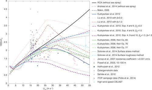
Figure 1 shows the results of some of the parameterisations described in Section 2. Different parameterisations give significantly different results, especially under very high wind speed conditions. According to a traditional parameterisation shown as a black line in Fig. 1 (from RCA4, see Section 4.1.1 for details), the drag coefficient increases with wind speed in the rough wind range. When the wind speed approaches 50, the drag coefficient is near 0.004, which is unrealistic. The new parameterisation of Andreas et al. (2014), which treats the friction velocity as a linear function of U _10N , produces an increasing drag coefficient until the wind speed is approximately 35ms⁻¹, after which it tends to saturation (dotted black line in Fig. 1). However, measurements indicate that C _d will decrease with increasing wind speed when the wind speed exceeds 30–35ms⁻¹.

The results of a parameterisation based on the limited-saturation layer (Makin, 2005) (Fig. 1, black dashed line) and its extension (Liu et al., 2012) for different wave age (Fig. 1, red dashed line for wave age β=1 and red dotted line for wave age β=0.2) agree reasonably well with measurements. However, there is a very sharp peak in the drag coefficient and no reasonable physical explanation of this feature. The new results of Soloviev et al. (2014) (Fig. 1, cyan line and cyan dashed line) agree well with the measurements from Jarosz et al. (2007) at wind speeds below 40ms⁻¹, but they overestimate the drag coefficient when compared with the data from Powell et al. (2003) and Holthuijsen et al. (2012). Using the conservation equation introduced the volume source of spray, as suggested by Kudryavtsev (Kudryavtsev, 2006; Kudryavtsev et al., 2012, shown in Fig. 1 as green and blue lines, respectively), the three SSGF parameterisations of Kudryavtsev (2006) are shown (green lines in Fig. 1). Changing the SSGF can greatly affect the results, but most SSGF parameterisations agree well with the measurements used here. The parameterisations taking account of sea spray influences perform better than those that do not in the data shown here. The sea-spray-influenced wind stress parameterisations can at least reproduce the reduced drag coefficient at high wind speeds (Fig. 1). The comparison shown in Fig. 1 indicates that the Kudryavtsev et al. (2012) results are better, as they show no sharp peak in drag coefficient. The recent results of Kudryavtsev et al. (2012) (dark blue line in Fig. 1) are used as the base parameterisation to add more wave information (i.e. the wave-age-dependent Charnock coefficient and the wave-state-dependent SSGF) to the parameterisation to investigate their influence.

Fig. 1 Various parameterised and measured drag coefficients (data were reproduced except Östergarnsholm data and Southern Ocean data). Red+signs are data measured from the ocean side of the air–sea interface (Jarosz et al., 2007); black squares are GPS dropsonde data (Powell et al., 2003); blue×signs are eddy-correlation data from Östergarnsholm for wind speeds over 15ms⁻¹ (Högström et al., 2008); black+signs are data from the Southern Ocean (Sahlée et al., 2012); cyan×signs are high wind speed CBLAST data (Bell et al., 2012); black×signs are typhoon data from the Pacific Ocean (Potter et al., 2014).

3.1.2. Improved wind stress parameterisation.

From comparing the use of different SSGFs in the Kudryavtsev (2006) parameterisation [green lines in Fig. 1 represent eqs. (65), (76) and (77) in Kudryavtsev, 2006], it can be seen that the drag coefficient is sensitive to the SSGF. The SSGF in Kudryavtsev et al. (2012) is related to friction velocity as the wind speed is the most important factor affecting SSGF. However, the SSGF is also related to many other environmental factors. As proposed by Toba et al. (2006), the development of wind waves, rather than wind speed, may be more appropriate to describe air–sea interaction conditions. Based on this idea, a non-dimensional parameter (the wind–sea Reynolds number, R_b ) was proposed to describe the air–sea transfer behaviour of spray (Toba et al., 2006; Zhao et al., 2006):7 $R_b=u_{*}^2/{\omega }_p\nu , \text{or}$7 8 $R_b=C_d\frac{u_{10}^3}{g\nu }{\beta }_w, {\beta }_w=\frac{g}{{\omega }_p{U}_{10}}$8

where ω_p is the wave angular frequency at the wind–sea spectral peak, ν the air kinematic viscosity, and β _w the wave age of wind waves. Zhao et al. (2006) proposed an SSGF dependent on the wind–sea wave Reynolds number for droplets with radii of 30–500 μm. To extend the SSGF to droplets with radii under 30 μm, we used the same method as Liu et al. (2011, 2012). Liu et al. (2012) introduced the whitecap coverage function into the SSGF of Monahan (1986) and developed a wind–sea Reynolds number-dependent SSGF for droplets smaller than 20 μm. In the range 20–30 μm, linear interpolation was used to fill the gap; the SSGF is then9 $\begin{array}{c}\frac{dF}{d{r}_0}=\{\begin{array}{c}0.506R_b^{1.09}{r}_0^{-2.95}(1+0.029r_0^{1.02})\times {10}^{1.19exp(-B_0^2)}\\ \hspace{1em}{r}_0<\mathrm{20\mu m}\\ 7.84\times {10}^{-3}{R}_b^{1.5}{r}_0^{-1}\mathrm{\hspace{1em}\hspace{1em}}30<r_0<75\mu \text{m}\\ 4.41\times {10}^1{R}_b^{1.5}{r}_0^{-3}\hspace{1em}75<r_0<200\mu \text{m}\\ 1.41\times {10}^{13}{R}_b^{1.5}{r}_0^{-8}\hspace{1em}200<r_0<500\mu \text{m}\end{array}\end{array}$9

where B ₀=(0.666−0.976×log(r ₀))/0.650. After the integral of the SSGFs in eq. (9), they are applied to eq. (5), which represents the basic parameterisation of Kudryavtsev et al. (2012), to investigate the impact of the SSGF on the drag coefficient.

As several researchers (e.g. Kumar et al., 2009) have recognised that the Charnock coefficient can be influenced by the wave state information, significant effort has been made to relate it to wave age. To investigate its influences under high wind speed conditions, we introduced the wave-age-dependent Charnock coefficient for the wind–sea condition from Carlsson et al. (2009) into the parameterisation in eq. (5),10 $\alpha =0.05{(c_p/u_{*})}^{-0.4}$10

Combining eqs. (5), (9) and (10), we obtain a new wind stress parameterisation that considers the wave-age-dependent Charnock coefficient and the wave-state-dependent SSGF. The impact on the drag coefficient of adding only the wave-state-dependent SSGF is shown in Fig. 1 (pink dashed–dotted line, β _w =0.2; pink dotted line, β _w =1.0). When the wave-age-dependent Charnock coefficient is added, this also changes the drag coefficient for the same wind wave age (dashed pink line in Fig. 1). When adding wave age as suggested, the impact on the drag coefficient is clearly significant.

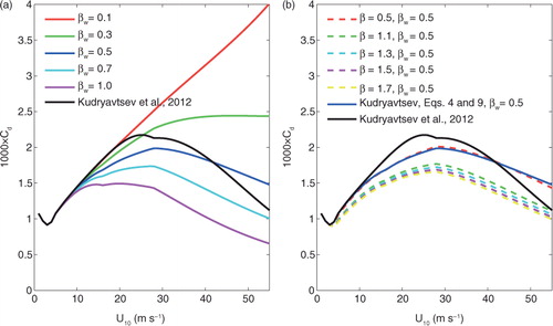
The impacts of the wave-dependent SSGF and wave-age-dependent Charnock coefficient on the drag coefficient are shown in more detail in Fig. 2. Both the SSGF and wave age can significantly influence the drag coefficient when the wind speed exceeds 15ms⁻¹. Figure 2a shows the results of introducing only the wave state impact on the SSGF. When the wind–sea is very young, the drag coefficient increases with the wind speed, because when the wind speed suddenly increases, the sea spray cannot develop immediately so it will not significantly affect the drag coefficient. When the wind wave age increases, the interaction between the wave and wind develops, and the influence of the sea spray on the drag coefficient will make it decrease with wind speed. If the SSGF is treated as a function of wind speed only, it cannot describe the wave state influence on the drag coefficient [see the blue line representing Kudryavtsev et al. (2012) in Fig. 2]. When the impact of wave age on the Charnock coefficient (using Carlsson et al., 2009) is also introduced, the results (Fig. 2b) indicate that the drag coefficient will decrease with increasing wave age. When the wave state is not very young (i.e. the wind wave age is approximately β _w >0.3), the drag coefficient will start to decrease at wind speeds of 25–30ms⁻¹, which is consistent with the results of Powell et al. (2003). The range of wave states studied here indicates that the wave state has a greater impact on SSGF than on the Charnock coefficient for the calculation of C_d .

Fig. 2 Comparison of wave state impact on the drag coefficient in the newly proposed parameterisation: (a) parameterisation with eqs. (5) and (9); (b) parameterisation with eqs. (5), (9) and (10).

3.2. Heat fluxes

Treating the interfacial latent and sensible heat fluxes, that is, H _L,int and H _S,int , as total fluxes is standard in most numerical models, as follows:11 $H_{S,int}={\rho }_a{c}_w{C}_S{U}_{10}(T_s-\theta )$11 12 $H_{L,int}={\rho }_a{L}_v{C}_E{U}_{10}(q_s-q)$12

where c _w is the seawater specific heat, C _S and C _E the transfer coefficients for the sensible and latent heat fluxes, respectively, L _v the latent heat of vapourisation for air, T _s the sea surface temperature (SST), θ the potential temperature at 10m, q _s the surface specific humidity, q the specific humidity at 10m. At high wind speeds, the spray-mediated heat fluxes are of comparable magnitude, as are the interfacial route heat fluxes. It is thus important to incorporate the spray-mediated heat fluxes into heat flux parameterisation.

Andreas et al. (2008) proposed a bulk air–sea flux algorithm that includes both the interfacial and spray routes for the latent and sensible heat fluxes. In a later study, Andreas et al. (2014) updated the algorithm to a new version that treats the latent, H _L,T and sensible H _S,T heat fluxes in the interfacial and spray routes separately:13 $H_{L,T}=H_{L,int}+H_{L,sp}$13 14 $H_{S,T}=H_{S,int}+H_{S,sp}$14

where H _L,int and H _s,int are calculated using the COARE algorithm (Fairall et al., 2003) and H _L,sp and H _S,sp are the sea-spray-mediated heat fluxes. Andreas (1992) found that spray droplets with radii of 10–300 μm contribute the most to the heat fluxes. At low air temperatures, the spray-sensible heat flux can be as great as the spray-latent heat flux. Based on earlier results Andreas et al. (2008, 2014) hypothesised that droplets with initial radii of 100 μm and 50 μm are good indicators of H _S,sp and H _L,sp , respectively. Then the sea-spray-mediated heat fluxes can be described as follows (Andreas et al., 2014):15 $H_{L,sp}={\rho }_w{L}_v\{1-{[\frac{r({\tau }_{f,50})}{50\mu m}]}^3\}{V}_L(u_{*,b})$15 16 $H_{S,sp}={\rho }_w{c}_w(T_s-T_{eq,100})V_S(u_{*,b})$16

where τ _f,50 is the residence time of droplets with a 50 μm initial radius and T _eq,100 the equilibrium temperature of droplets with a 100 μm initial radius. Based on measurements, the wind functions of V_L (u _*,b ) and V_S (u _*,b ) are17 $V_L=\{\begin{array}{c}1.76\times {10}^{-9}\mathrm{\hspace{1em}\hspace{1em}}0\le u_{*,b}\le 0.1358 m{s}^{-1}\\ 2.08\times {10}^{-7}{u}_{*,b}^{2.39}\mathrm{\hspace{1em}\hspace{1em}}0.1358 m{s}^{-1}\le u_{*,b}\end{array}$17 18 $V_S=\{\begin{array}{c}3.92\times {10}^{-8}\mathrm{\hspace{1em}\hspace{1em}}0\le u_{*,b}\le 0.1480 m{s}^{-1}\\ 5.02\times {10}^{-6}{u}_{*,b}^{2.54}\mathrm{\hspace{1em}\hspace{1em}}0.1480 m{s}^{-1}\le u_{*,b}\end{array}$18

to keep the spray flux algorithm reliable, the bulk friction velocity, u _*,b , is calculated using the method described by Andreas et al. (2014), which is linearly related to U _10N .

4. Coupled model system and measurements

4.1. Coupled system

4.1.1. RCA.

The RCA version 4 atmospheric model developed at the Swedish Meteorological and Hydrological Institute (SMHI) is used in the coupled system. It is a hydrostatic model incorporating terrain-following coordinates and semi-Lagrangian, semi-implicit calculations. The domain of the RCA model used here includes all of Europe (see Fig. 3). The resolution is 0.22° spherical with a rotated latitude/longitude grid. There are 40 vertical levels, the lowest model level being approximately 32m above mean sea level, and the time step is 15 min. The ERA-40 data (Uppala et al., 2005), which constitute ECMWF reanalysis data, provide the boundary and initial field information for RCA, which takes account of SST, ice cover, wind speed, and so on.

The wind stress parameterisation in RCA is calculated based on the roughness length, z ₀, which is described as follows in RCA:19 $z_0=f(U)\times \alpha \frac{u_{*}^2}{g}+[1-f(U)]\times 0.11\frac{\nu }{u_{*}}$19

Fig. 3 The domain of the RCA model used in this study (red box area); the red×is the FINO1 site; the blue box area is the area shown in Figs. 17 and 18; the blue×indicates the centre of storm Uill at time 2012-01-03:12 (discussed in Section 6.3).

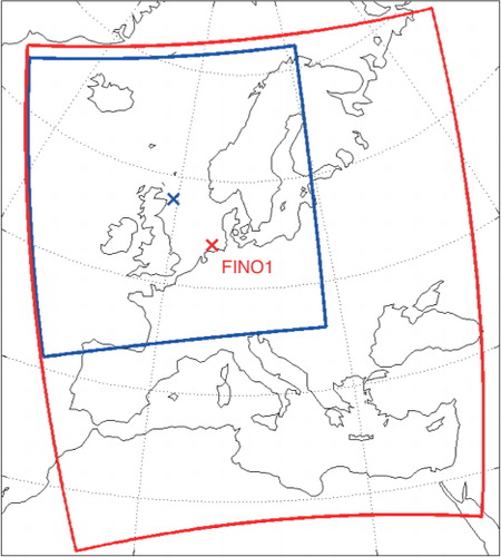
where α is set to 0.0185 in this study and f(U) is a wind speed function responsible for the transition between smooth and rough flows. The coupled RCA–WAM system is similar to that described by Rutgersson et al. (2010, 2012).

4.1.2. WAM.

The third-generation, full-spectral wave model WAM (WAMDI, 1988) is used in the coupled system. In the WAM model, the spectral energy balance equation is used to describe the 2D wave spectrum. In this study, the resolution and domain of WAM are the same as in the RCA model. The input data for wind speed at 10m are from the RCA model every time step (time step in WAM is same as in RCA, 15 min). For simplicity, the lateral wave boundary condition is not introduced in this study; this will have only a minor impact in high wind conditions. In WAM, parameters such as significant wave height, peak wind wave period and roughness length, z ₀, are computed from the 2D spectrum. In the coupled model, the WAM model provides the wave information for RCA.

4.1.3. Coupled experiments.

To investigate the influence of sea spray on storm simulations, six experiments are designed. The wind stress and heat flux parameterisations of these experiments are listed in Table 1.

As control experiments, the original RCA model was used in Exp-1 to simulate storms. The only difference between Exp-1 and Exp-4 is in their wind stress parameterisations. Inter-comparison in this group evaluates the impact of sea spray and wave state on the simulation results. Exp-2 is the base wind stress parameterisation in which SSGF is related only to friction velocity. Exp-3 uses the wave-state-dependent SSGF; Exp-4 uses both the wave-state-dependent SSGF and wave-age-dependent Charnock coefficient.

In addition, Exp-1, Exp-4, Exp-5 and Exp-6 are compared to test the separate influences of sea spray on the wind stress and heat fluxes. In Exp-5, only the sea spray impact on the heat fluxes is introduced. Exp-6 is the full coupled model, in which the sea spray impacts on both the wind stress and heat fluxes are considered in order to investigate the sea spray influence.

Table 1. Wind stress and heat fluxes parameterisations for the various simulations

Experiments	Wind stress	Heat fluxes	Notes
Exp-1	Eq. (19)	RCA	Basic experiments
Exp-2	Eqs. (5) and (6)	RCA	Basic sea spray parameterisation
Exp-3	Eqs. (5) and (9)	RCA	Wave-state-dependent SSGF impact on wind stress
Exp-4	Eqs. (5), (9) and (10)	RCA	Wave-state-dependent SSGF and impact on wind stress
Exp-5	Eq. (19)	Andreas et al., 2014	Sea spray impact on heat fluxes
Exp-6	Eqs. (5), (9) and (10)	Andreas et al., 2014	Full coupled case (Exp-4+Exp-5)

4.2. Measurements

In this study, the FINO1 data are used to verify the model results. The FINO1 offshore platform (54°00′53.5″N, 6°35′15.5″E) is located 45km north of Borkum Island in the North Sea. A 100-m-tall mast is instrumented to measure the wind speed, wind direction, pressure and relative humidity at multiple levels. Wind speed is measured at eight levels (from approximately 33 to 100 m) using cup anemometers. Wind vanes are installed at 33, 50, 70 and 90m to measure the wind direction. Air temperature is measured at 33, 40, 50, 70 and 100m and air humidity at 20 and 100 m. FINO1 faces rather open ocean conditions in the north and west and stands in water 30m deep. Further details about the platform can be found in Neumann and Nolopp (2007).

5. Storm cases

Six storms (named Gero, Erwin/Gudrun, Kyrill, Ulli, Patrick and Klaus) are used to test these parameterisations including sea spray influence in the RCA–WAM coupled system. The related information about the six storms [i.e. track, minimum sea level pressure (MSLP), and maximum wind speed at 925 hPa] are obtained from the Extreme Wind Storms (XWS) Catalogue, in which storms are tracked using the ERA-Interim dataset. For detailed information about these data, please see www.europeanwindstorms.org/.

Gero, a severe Atlantic storm, was generated on 7 January and dissipated on 14 January 2005. On 11–12 January, Gero passed northwest of Ireland and north of Scotland, causing a record wind speed of 45.2ms⁻¹ in Stornoway, Scotland. The MSLP according to the ERA-Interim reanalysis is 947.8 hPa recorded at 63°W, 60.4°N, at 0:00 12 January.

A second storm hit Europe in January 2005; it is called Erwin (named by the Free University of Berlin) or Gudrun (named by the Norwegian Meteorological Institute). Gudrun/Erwin developed in a frontal zone south of Newfoundland and then passed over the central North Atlantic. The storm moved into the Baltic Sea on 9 January, with an MSLP of 960 hPa. As Gudrun/Erwin continued to move eastward, it slowed down and dissipated over Russia.

Kyrill was generated over Newfoundland on 15 January 2007, crossed the Atlantic Ocean, passed Ireland, crossed the North Sea, and made landfall in Germany and the Netherlands on 18 January. Its winds reached hurricane strength, and the maximum wind speed over land was 36.4ms⁻¹ at 925 hPa according to the ERA-Interim reanalysis and the minimum mean sea level pressure was 961.1 hPa.

Ulli formed on 2 January and dissipated on 11 January 2012. During its life, it crossed the Atlantic Ocean, North Sea and Baltic Sea, causing severe damage in the United Kingdom. ERA-Interim reanalysis data indicate that the minimum mean sea level pressure was 954.3 hPa at 1.8°E, 58.7°N. The maximum wind speed at 925 hPa over land was 36.3ms⁻¹.

Patrick (Dagmar) was generated on 24 December 2011 as a weak low just south of Newfoundland. Patrick caused severe damage in the central coastal areas, continuing over the Scandinavian Peninsula towards the Baltic Sea and Gulf of Finland. The minimum mean sea level pressure was 953.9 hPa at 17.4°W, 61.2°N. The maximum wind speed at 925 hPa over land was 30.08ms⁻¹.

Klaus is a windstorm, which made landfall over southern France, Spain and parts of Italy on January 2009. The storm generated in the Bay of Biscay and then moved to the south-eastward though France. The minimum mean sea level pressure was 966.0 hPa at 7.3°W, 46.5°N.

6. Results

6.1. Comparison with FINO1 measurements

To verify the model performance when introducing the parameterisations into the coupled model system, the results from the nearest grid point in the model are compared with FINO1 hourly data. Four statistical parameters are used in this study: the bias or mean error (ME), mean absolute error (MAE), root mean square error (RMSE) and Pearson correlation coefficient (R). When the comparison group data comprise fewer than 30 samples, the results are not used.

6.1.1. Wind stress parameterisation comparison.

The simulation results of Exp-1 to Exp-4 for wind speed, wind gradient and temperature are compared with measurements from FINO1. Time series of wind speed at 33m are shown in Fig. 4, statistical data in Table 2, and wind speed range statistics in Fig. 5 to investigate the performance of the parameterisations for different wind speed ranges.

When including the sea spray impact on the wind stress, the statistics do not improve over the whole wind speed range for any of the experimental set-ups (Table 2). However, the various wind stress parameterisations including the sea spray impact generally capture the high wind peaks better. Inter-comparison of Exp-1 to Exp-4 indicates that there is a small impact when including only the SSGF parameterisation of Kudryavtsev et al. (2012) in Exp-2; the impact is larger when including the wave-state-dependent SSGF in Exp-3; the ME is reduced by up to 1ms⁻¹ for the high wind speed ranges when the wave-age-dependent Charnock coefficient and SSGF are introduced in Exp-4. Of Exp-1 to Exp-4 (Fig. 4), Exp-4 best captures the high wind peaks. In the range of 16–24ms⁻¹, the ME is reduced by 0.72ms⁻¹ (78%) and 0.75m s⁻¹ (82%) in Exp-3 and Exp-4, respectively; the MAE is reduced by 0.17ms⁻¹ (12%) and 0.15ms⁻¹ (10%) in Exp-3 and Exp-4, respectively; and the RMSE is reduced by 0.13ms⁻¹ (7%) and 0.12ms⁻¹ (6%) in Exp-3 and Exp-4, respectively. Introducing the wave-state-dependent SSGF (Exp-3) has a greater impact on the results than does introducing the wave-age-dependent Charnock coefficient (see Fig. 5). When comparing wind measurements at other platform heights, the results are similar. There are minor differences in the wind gradient between the 100-m and 33-m measurements in the different experiments (results not shown). When the sea spray influence on the wind stress is considered, the model performance will worsen slightly for temperature (data from 100m are shown in Table 3).

Fig. 4 Modelled wind speed results compared with FINO1 measurements at a height of 33 m: (a) January 2005, (b) January 2007 and (c) January 2012.

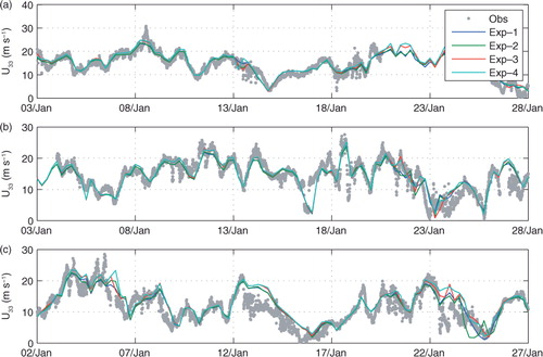
Fig. 5 Statistical results for wind speed measured at a height of 33m (a) mean error, (b) mean absolute error and (c) root mean square difference.

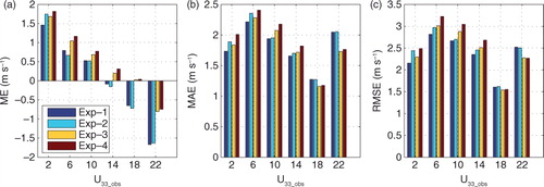
Table 2. Comparative statistics for the wind speed results at a height of 33 m; bias or mean error (ME), mean absolute error (MAE), root mean square error (RMSE) and Pearson correlation coefficient (R)

	Exp-1	Exp-2	Exp-3	Exp-4	Exp-5	Exp-6
ME	0.13	0.09	0.47	0.56	0.20	0.62
MAE	1.83	1.88	1.86	1.95	1.85	2.03
RMSE	2.47	2.55	2.59	2.74	2.53	2.79
R	0.88	0.87	0.87	0.86	0.87	0.86

Table 3. Comparative statistics for the temperature results at a height of 100m; bias or mean error (ME), mean absolute error (MAE), root mean square error (RMSE) and Pearson correlation coefficient (R)

	Exp-1	Exp-2	Exp-3	Exp-4	Exp-5	Exp-6
ME	−0.59	−0.58	−0.65	−0.68	−0.44	−0.41
MAE	0.99	0.99	1.04	1.06	0.87	0.87
RMSE	1.40	1.40	1.44	1.45	1.31	1.31
R	0.87	0.87	0.86	0.87	0.87	0.87

Table 4. Comparative statistics for the different wind speed range results at a height of 33 m; bias or mean error (ME), mean absolute error (MAE) and root mean square error (RMSE)

m s^−1	0–4	4–8	8–12	12–16	16–20	20–24
ME
Exp-1	1.46	0.79	0.52	−0.08	−0.65	−1.67
Exp-4	1.82	1.16	0.78	0.31	0.04	−0.75
Exp-5	1.72	1.02	0.55	−0.06	−0.68	−1.57
Exp-6	1.87	1.14	0.79	0.42	0.16	−0.55
MAE
Exp-1	1.73	2.22	1.94	1.66	1.27	2.05
Exp-4	2.01	2.41	2.18	1.82	1.17	1.76
Exp-5	1.88	2.27	1.83	1.74	1.35	2.06
Exp-6	2.03	2.61	2.09	1.87	1.50	1.75
RMSE
Exp-1	2.15	2.82	2.67	2.35	1.61	2.52
Exp-4	2.49	3.23	3.04	2.68	1.56	2.27
Exp-5	2.45	2.94	2.53	2.51	1.73	2.58
Exp-6	2.61	3.32	2.98	2.65	1.99	2.31

6.1.2. The co-impact of sea spray wind stress and heat fluxes.

Adding only the sea spray impact on the heat fluxes only slightly influences the wind speed in the high wind speed range compared with the control experiment. However, the wind speed will increase if only the sea spray influence on the wind stress is taken into account (Exp-4). If the sea spray impacts on both the wind stress and the heat fluxes (Exp-6) are included, the simulations perform better in terms of ME, MAE and RMSE than if only one impact is introduced (Exp-4 and Exp-5) in the high wind speed range (20–24ms⁻¹) (Table 4).

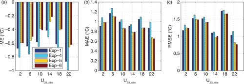
In general, the modelled air temperature will decrease slightly if only the sea spray impact on wind stress is considered (see Exp-4 in Figs. 6 and 7). In contrast, if the sea spray impact on heat fluxes in introduced, the air temperature will increase (especially in the high wind speed range, the temperature error is reduced by more than 0.2°C in terms of ME and MAE; see Exp-5 in Fig. 7). Adding both influences (Exp-6) improves the model's temperature performance, increasing the temperature (see Fig. 6). According to the statistical results in terms of ME, MAE, RMSE and R (see Table 3 and Fig. 7), if the sea spray impact on both the heat fluxes and wind stress are added (Exp-6), the model's temperature performance will be better than if only one influence is added.

Fig. 6 Same as in Fig. 4, but for temperature measured at a height of 100m compared with the second model layer (about 100 m).

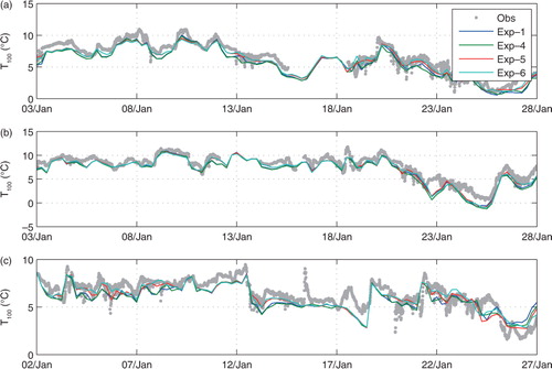
Fig. 7 Statistical results for temperature measured at a height of 100 m: (a) mean error, (b) mean absolute error and (c) root mean square difference.

6.2. Storm tracks and intensity

6.2.1. Storm tracks.

The simulated storm tracks, defined from the minimum sea level pressure, are compared with the observations in Fig. 8, while a summary of the MAE analysis of the storm tracks is presented in Table 5. The simulated storm tracks generally appear to be consistent with the observations. However, all experiments perform poorly when the storms suddenly change their heading direction, as storms Gero and Ulli did. The different wind stress parameterisations only slightly influence the storm tracks. If only the sea spray impact on the heat fluxes is considered in the coupled model (Exp-5), the impact is slightly larger, and the tracks of most storms will be somewhat better simulated (however still not significantly). Considering the sea spray influence on both stress and heat fluxes, it has only little effect on the storm tracks (even little worse than Exp-5).

Fig. 8 The storm tracks represented by the minimum sea level pressure every three hours: (a) Gero, (b) Erwin/Gudrun, (c) Kyrill, (d) Ulli, (e) Patrick and (f) Klaus.

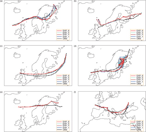
Table 5. The mean absolute error (MAE) of the minimum sea level pressure centre (km)

	Exp-1	Exp-2	Exp-3	Exp-4	Exp-5	Exp-6
Gero	187.92	189.86	182.32	150.99	170.48	184.31
Erwin	172.49	174.53	174.34	172.85	174.91	180.54
Kyrill	106.56	110.58	119.84	131.80	101.88	132.21
Ulli	250.64	265.42	254.23	259.64	230.51	199.48
Patrick	193.08	245.76	197.37	197.88	194.17	186.84
Klaus	266.72	270.49	251.58	250.69	268.47	269.11
Average	196.23	209.44	196.61	193.98	190.07	192.08

6.2.2. Minimum sea level pressure.

The temporal development of the MSLP of storms is shown in Fig. 9 and the related MAEs are shown in Table 6. Comparing simulations using different wind stress parameterisations (Exp-1 to Exp-4) indicates that all experiments underestimate the intensity of the storms. Introducing only a non-wave-state-dependent SSGF has a minor impact on the storm simulations (Exp-2). When a wave-state-dependent SSGF is introduced into the wind stress parameterisation of Kudryavtsev et al. (2012) (Exp-3), the storm is intensified and the MSLP simulation improves. The simulation improves further by adding the wave-age-dependent Charnock coefficient (Exp-4). Exp-4 is the best one when compared with the reanalysis data, which can reduce the MSLP error by approximately 11% on average compared with Exp-1.

Including the impact of sea spray in the heat flux parameterisation has a smaller effect, but it can still reduce the error of MSLP by approximately 7% compared with the error in Exp-1. When the sea spray impacts on both the wind stress and heat fluxes are added, the simulated MSLP results improve significantly, with an average 23% reduction of the error from Exp-1 (see Table 6).

Fig. 9 The minimum sea level pressure of different storms over time: (a) Gero, (b) Erwin/Gudrun, (c) Kyrill, (d) Ulli, (e) Patrick and (f) Klaus.

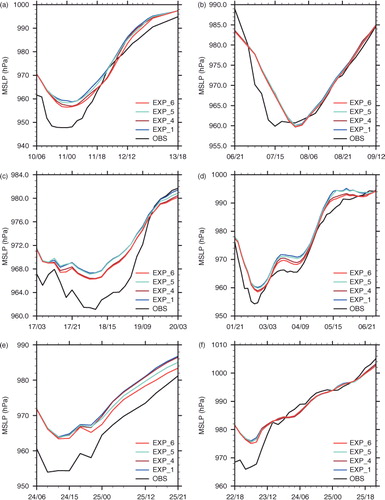
Table 6. The mean absolute error (MAE) of the minimum sea level pressure (hPa)

	Exp-1	Exp-2	Exp-3	Exp-4	Exp-5	Exp-6
Gero	6.62	6.41	5.78	5.69	6.10	5.06
Erwin	2.45	2.43	2.35	2.36	2.35	2.16
Kyrill	3.67	3.65	3.33	3.28	3.72	3.21
Ulli	3.78	3.65	2.99	2.68	3.51	2.28
Patrick	7.61	7.70	6.83	7.27	6.54	5.33
Klaus	2.58	2.60	2.58	2.53	2.53	2.41
Average	4.45	4.41	3.98	3.97	4.12	3.41

6.2.3. Maximum wind speed.

The time series of maximum wind speed at 925 hPa for the six storm cases are shown in Fig. 10 and the related MAEs are shown in Table 7. The performances of the different wind stress parameterisations are similar to the MSLP performance, as the parameters are strongly linked. In Exp-4, the maximum wind speed error is reduced by an average of approximately 17%. When letting the sea spray influence the heat fluxes only, the model results improve only slightly. Introducing the sea spray influence on both heat fluxes and wind stress yields the best maximum wind speed performance, reducing the error by an average of 23% from that of Exp-1. The significant influences on the maximum wind speed are exerted mainly during the periods of highest wind speed.

Fig. 10 The maximum wind speed at 925 hPa of different storms over time: (a) Gero, (b) Erwin/Gudrun, (c) Kyrill, (d) Ulli, (e) Patrick and (f) Klaus.

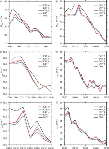
Table 7. The mean absolute error (MAE) of the maximum wind speed at 925 hPa (ms⁻¹)

	Exp-1	Exp-2	Exp-3	Exp-4	Exp-5	Exp-6
Gero	4.58	4.12	3.41	3.34	4.38	3.34
Erwin	2.96	2.93	2.54	2.52	3.12	2.53
Kyrill	2.16	2.14	1.79	1.82	2.11	1.66
Ulli	1.71	1.69	1.81	1.97	1.53	1.98
Patrick	3.86	3.71	2.81	2.93	3.43	2.40
Klaus	1.76	1.70	1.59	1.57	1.54	1.24
Average	2.84	2.72	2.32	2.36	2.68	2.19

6.3. Storm structure

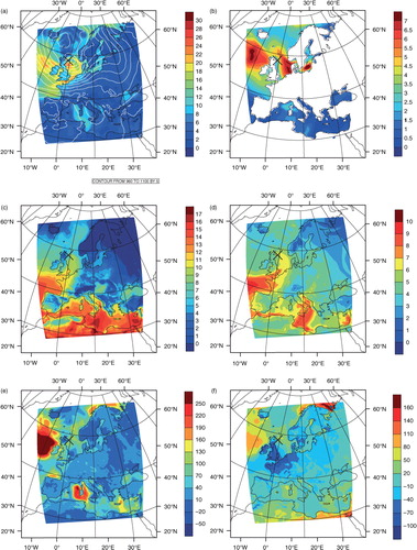
In this section, one time step from storm Uill (2012-01-03:12) is used to illustrate the influence of the sea spray on the storm structure. The general impact of changes in the various parameterisations is similar in the development of all storms. The minimum pressure in this situation is approximately 945 hPa and maximum wind speed at 925 hPa exceeds 30m s⁻¹. The sea level pressure, 10-m wind speed, significant wave height, temperature, humidity and heat fluxes are all shown in Fig. 11.

Fig. 11 The simulation results from the control experiment (Exp-1) at time 2012-01-03:12: (a) wind speed (m s⁻¹) at 10m and sea level pressure (h Pa), (b) significant wave height (m), (c) air temperature at 2m (°C), (d) humidity at 2m (g kg⁻¹), (e) latent heat flux (W m⁻²) and (f) sensible heat flux (W m⁻²). The black×is the centre of the storm in this time step.

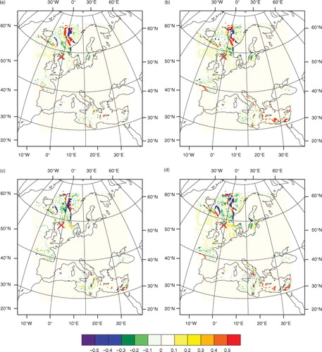
Figures (12–16) show the differences between Exp-1 and Exp-3 to Exp-6 for sea level pressure, wind speed at 10m, heat flux, wave age and wind wave age at time 2012-01-03:12, respectively. Exp-2 is not shown as the differences are small when including only the wind stress parameterisation of Kudryavtsev et al. (2012). Introducing the sea state impact on the SSGF and the Charnock coefficient (Exp-3 and Exp-4) into the parameterisation of Kudryavtsev et al. (2012) intensifies the storms, as was also seen in Figs. 9 and 10, lowering the sea level pressure and an increasing the wind speed. If only the sea spray impact on wind stress is introduced, the heat flux is only slightly increased due to the increased wind speed (Fig. 14). However, considering the sea spray heat flux (Exp-5) significantly changes the heat flux (up to 70Wm⁻²) in the high wind speed area. If the sea spray impacts on both wind stress and heat fluxes are considered (Exp-6), the heat flux will increase by more than 80Wm⁻² in high wind speed areas. Considering sea spray impacts on both heat fluxes and wind stress (Exp-6) will increase the wind speed by more than 2ms⁻¹ in some high wind speed areas. When considering the impact of sea spray, it changes the wave age and wind wave age significantly (see Figs. 15 and 16). The spatial pattern of wave age and wind wave age is also different.

Fig. 12 Difference in sea level pressure (hPa) from that of Exp-1 at time 2012-01-03:12: (a) Exp-3 – Exp-1, (b) Exp-4 – Exp-1, (c) Exp-5 – Exp-1 and (d) Exp-6 – Exp-1. The red×is the centre of the storm in this time step.

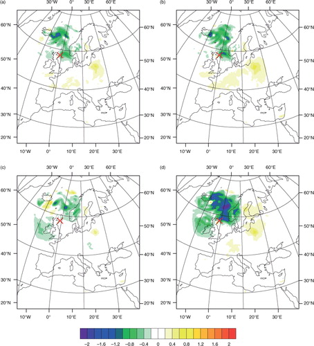
Fig. 13 Difference in wind speed at 10m (m s⁻¹) from that of Exp-1 at time 2012-01-03:12: (a) Exp-3 – Exp-1, (b) Exp-4 – Exp-1, (c) Exp-5 – Exp-1 and (d) Exp-6 – Exp-1. The red×is the centre of the storm in this time step.

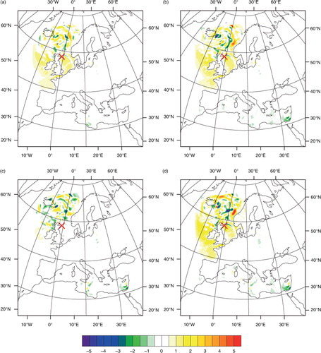
Fig. 14 Difference in heat flux (i.e. sensible heat flux and latent heat flux) (W m⁻²) from that of Exp-1 at time 2012-01-03:12: (a) Exp-3 – Exp-1, (b) Exp-4 – Exp-1, (c) Exp-5 – Exp-1 and (d) Exp-6 – Exp-1. The red×is the centre of the storm in this time step.

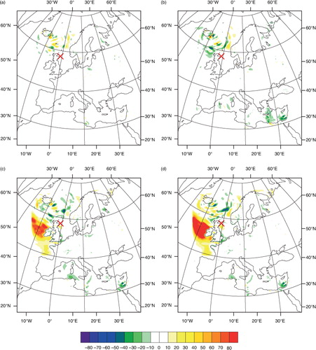
Fig. 15 Difference in wave age from that of Exp-1 at time 2012-01-03:12: (a) Exp-3 – Exp-1, (b) Exp-4 – Exp-1, (c) Exp-5 – Exp-1 and (d) Exp-6 – Exp-1. The red×is the centre of the storm in this time step.

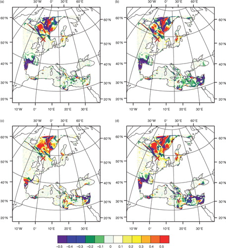
Fig. 16 Difference in wind wave age from that of Exp-1 at time 2012-01-03:12: (a) Exp-3 – Exp-1, (b) Exp-4 – Exp-1, (c) Exp-5 – Exp-1 and (d) Exp-6 – Exp-1. The red×is the centre of the storm in this time step.

The humidity and temperature structures of the storm in the same time step of Exp-1 are shown in Figs. 17 and 18. Point (0, 0), the centre of the storm in this time step, is shown in the blue box area in Fig. 3. In this time step, high-speed wind take high-humidity and high-temperature air from the south-west of the storm centre to maintain the intensity of the storm.

Fig. 17 Difference in humidity from that of Exp-1 at different heights at time 2012-01-03:12: (a) Exp-1, (b) Exp-4 – Exp-1, (c) Exp-5 – Exp-1 and (d) Exp-6 – Exp-1.

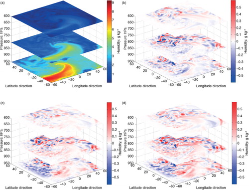
Fig. 18 Difference in temperature from that of Exp-1 at different heights at time 2012-01-03:12: (a) Exp-1, (b) Exp-4 – Exp-1, (c) Exp-5 – Exp-1 and (d) Exp-6 – Exp-1.

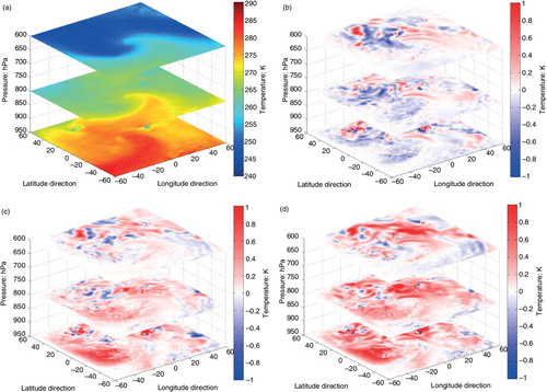
Considering the sea spray influence on the momentum flux slightly increases the humidity, even at higher levels (Exp-4). In the 800 hPa and 600 hPa layer, Exp-4 has lower air temperatures than does Exp-1 in most areas (see Fig. 18). Considering only the sea spray impact on the heat fluxes (Exp-5) will increase the air humidity in front and to the right of the storm centre and reduce the air humidity behind the storm centre in the lower 950 hPa layer. As the height increases, the influence on the humidity decreases (see Fig. 17). For temperature structure (Fig. 18), the sea spray impact on heat fluxes will increase the air temperature by approximately 0.3°C in most areas at a height of 800 hPa. At a height of 600 hPa, the temperature is still over 0.1°C higher than in Exp-1.

The differences between the full coupled simulation (i.e. including the sea spray impact on both wind stress and heat fluxes) and Exp-1 are also shown in Figs. 17 and 18. The influence pattern is similar to that of Exp-6 (i.e. including only sea spray impact on heat fluxes), but the influence is stronger. The temperature is over 0.5° higher than that in Exp-1 in most of the areas at 800 hPa.

7. Discussion

In this study, sea spray influence on the development of storms is investigated in an atmosphere–wave coupled model incorporating a proposed sea spray influence drag coefficient parameterisation and the heat flux parameterisation of Andreas et al. (2014). Introducing only the SSGF parameterisation of Kudryavtsev et al. (2012) has a relative small effect on the simulation. It is only when also introducing the wave state impact on the SSGF and the wave-age-dependent Charnock coefficient that the effect on the simulated storm intensity increases (Exp-3 and Exp-4). The best model performance is observed in the setup including the sea spray influence on both wind stress and surface heat fluxes (Exp-6), which increases the air temperature and intensifies the storms.

As expected, the wind stress parameterisations including sea spray influence can improve the model performance in the high wind speed range, but the model performs worse in the low wind speed range relative to the FINO1 data. One possible explanation is that swell conditions usually arise at low wind speeds. The existence of swell will influence the turbulence in the near-surface layer. The swell waves and airflow form a very complex interaction with increasing or decreasing stress depending on a variety of parameters, including wave state, wave height and direction differences between waves and wind (i.e. Donelan et al., 1997; Drennan et al., 1999; Kudryavtsev and Makin, 2004; Högström et al., 2009). These effects are not included in the suggested parameterisation and the model can thus not be expected to perform well in low wind conditions.

The new parameterisations including sea spray impact add some biases to the wind speed in the intermediate wind speed range. This may be caused by the underestimation of the drag coefficient in the intermediate wind speed range when the wave age and wind wave age is large (see Fig. 2). The SSGFs used in this study is adapted from Zhao et al. (2006), which is based on limited amount of measurements. There may be some uncertainness in the SSGFs, which cause the increased biases in the intermediate wind speed range compared to the control experiment (Exp-1).

Inter-comparison between the six experiments indicates that wind stress parameterisations including sea spray intensify the storms (in terms of wind speed and minimum pressure). When the sea spray impact on the wind stress is considered, the drag coefficient will decrease, transporting less energy to the ocean and leaving more energy in the atmosphere. This will lead to intensified storms in the simulations. The decreasing drag coefficient at high wind speeds will reduce the transfer coefficients of sensible and latent heat fluxes, in turn reducing the heat fluxes. In this respect, the sea spray influence on the wind stress will reduce the air temperature, as also observed in the simulations. Introducing sea spray impact on the heat fluxes will increase the heat fluxes transported from ocean to atmosphere and increase the air temperature. This also can be seen in the structure of the humidity and temperature (Figs. 17 and 18). Adding the sea-spray-mediated heat fluxes has the same effect as the increase of the heat transfer via increase of the temperature roughness scale, as suggested by Kudryavtsev et al. (2012).

If the impacts of sea spray on both wind stress and heat fluxes are considered (Exp-6), it overestimates the wind speed in some time periods compared to FINO1 data. Thus Exp-6 adds more biases to the wind speed simulation compared to Exp-4. One possible reason for the biases is that the resolution of the model is not high enough to capture the wind speed change in the simulations. When a decrease of drag coefficient and increase of heat transfer were implemented into the numerical simulation in the study of Zweers et al. (2015), the intensity of the tropical cyclones was overestimated. Sensitivity experiments show that the changes of SST have a big impact on the intensity of tropical cyclones. This may also explain the overestimation of wind speed in some periods in our simulation of mid-latitude storms in Exp-6 because the changes of SST are not considered in this study. The decrease of the drag coefficient reduces the heat transfer coefficient. However, the increase of the wind speed caused by the decrease of drag coefficient increases the sea-spray-mediated heat fluxes. The co-impact of the two functions, i.e., sea spray impact on wind stress and heat fluxes, make that the temperature simulation of Exp-6 has the best performance in the simulation of the temperature.

Including sea spray in the heat flux parameterisation (Exp-5) is little more important than the wind stress for the storm tracks (both of them have little effect), improving them to some extent. One possible reason for this improvement is that more energy (heat) will be transported to the atmosphere in the high wind speed area, which is not symmetrical around the storm centre. This unsymmetrical energy increase (due to sea spray heat fluxes in the high wind speed areas) will make the storm centre shift in the direction with more energy. The sea spray heat fluxes can also provide energy for storm development.

Introducing the sea spray impact on wind stress does not improve the storm track significantly. One possible reason for this insignificant improvement is that the studied domain covers Europe (i.e. is dominated by land areas), so the storm centres are not located over the ocean surface for extended time periods. The impact of the wind stress parameterisation over the sea may not be enough to change the storm tracks to any great extent.

The main limitation when parameterising sea spray is the limited data at very high wind speeds. Because of the limited data, we use the parameterisation of Kudryavtsev et al. (2012) based on the agreement with the measurements used in this paper. The formulation is expanded to include the impact of the wave state on the SSGF and the Charnock coefficient.

8. Summary and conclusions

Measurements made in the field and laboratory indicate that sea spray plays an important role in momentum and heat fluxes. At high wind speeds, most studies demonstrate that the drag coefficient decreases with increasing wind speeds (e.g. Powell et al., 2003). In addition, the sea-spray-mediated heat fluxes are larger than the interfacial heat fluxes (i.e. Andreas and Emanuel, 2001; Andreas et al., 2008). In the present study, a new wind stress parameterisation is proposed based on the parameterisation of Kudryavtsev and Makin (2011) and Kudryavtsev et al. (2012). The wave-state-dependent SSGF (Zhao et al., 2006) and wave-age-dependent Charnock coefficient (Carlsson et al., 2009) are introduced into the proposed wind stress parameterisation. The wind stress parameterisations and heat flux parameterisations at high wind speeds are applied to an atmosphere–wave coupled model to simulate several storm cases for the comparison of the wind stress parameterisations and their co-impact with the sea spray influence on the development of storms.

Introducing the wave-state-dependent SSGF into the wind stress parameterisation improves the model results at high wind speeds. The newly proposed parameterisation increases the high wind speeds but reduces the air temperature relative to the control experiment. The most important component of the new parameterisation is the wave dependence of the SSGF. Based on the measurements, this component improves the models wind speed performance but degrades the air temperature performance. If the sea spray impacts on both the wind stress and heat fluxes are considered, the model will perform the best not only for temperature, but also for wind speed.

As expected, the wind stress parameterisation including the sea spray influence intensifies the storms in terms of MSLP and maximum wind speed. Adding only the sea spray impact on heat fluxes to the parameterisation causes minor changes in the storm intensity and the storm tracks. Including sea spray heat fluxes can increase the humidity and temperature in storms; in contrast, including the sea spray impact on wind stress will reduce the humidity and temperature (Figs. 17 and 18).

From the simulation results, we conclude that the influence of sea spray on storm development is important and should be taken into account in numerical models. The study includes one coupled model and six storms, which can be considered too limited to support more generalised conclusions. One can, however, generally expect slightly more intense storms in coupled models when taking the effects of waves and sea spray into account. It is also important to introduce the wave impact on the SSGF (and on the Charnock coefficient) as well as the sea spray impact on heat fluxes. The uncertain physical mechanism underlying the sea spray impacts on the wind stress and heat fluxes should be further studied to obtain better parameterisations for numerical models. In addition, the details of the sea spray impact on the storm structure should be studied to learn more about the mechanism in operation.

9. Acknowledgements

Lichuan Wu is supported by the Swedish Research Council (project 2012-3902). Xiaoli Guo Larsén thanks the EU Marina and Mermaid projects for access to the FINO1 data. Markus Meier and Christian Dieterich at SMHI are acknowledged for providing access to and technical support with the RCA model.

References

- Andreas E. L . Sea spray and the turbulent air–sea heat fluxes. J. Geophys. Res. Oceans (1978–2012). 1992; 97(C7): 11429–11441.
- Andreas E. L . Spray stress revisited. J. Phys. Oceanogr. 2004; 34(6): 1429–1440.
- Andreas E. L. , Emanuel K. A . Effects of sea spray on tropical cyclone intensity. J. Atmos. Sci. 2001; 58(24): 3741–3751.
- Andreas E. L. , Mahrt L. , Vickers D . An improved bulk air–sea surface flux algorithm, including spray-mediated transfer. Q. J. Roy. Meteorol. Soc. 2014; 141: 642–654.
- Andreas E. L. , Persson P. O. G. , Hare J. E . A bulk turbulent air–sea flux algorithm for high-wind, spray conditions. J. Phys. Oceanogr. 2008; 38(7): 1581–1596.
- Barenblatt G . Similarity. Self-Similarity, and Intermediate Asymptotics. 1979; Consultants Bureau, New York.
- Barenblatt G., Chorin A., Prostokishin V. A note concerning the lighthill sandwich model of tropical cyclones. Proc. Natl. Acad. Sci. U.S.A. 2005; 102(32): 11148–11150.
- Barenblatt G. , Golitsyn G . Local structure of mature dust storms. J. Atmos. Sci. 1974; 31(7): 1917–1933.
- Bell M. M. , Montgomery M. T. , Emanuel K. A . Air–sea enthalpy and momentum exchange at major hurricane wind speeds observed during CBLAST. J. Atmos. Sci. 2012; 69(11): 3197–3222.
- Carlsson B. , Rutgersson A. , Smedman A.-S . Impact of swell on simulations using a regional atmospheric climate model. Tellus A. 2009; 61(4): 527–538.
- Charnock H . Wind stress on a water surface. Q. J. Roy. Meteorol. Soc. 1955; 81(350): 639–640.
- Donelan M. , Haus B. , Reul N. , Plant W. , Stiassnie M. , co-authors . On the limiting aerodynamic roughness of the ocean in very strong winds. Geophys. Res. Lett. 2004; 31(18): L18306.
- Donelan M. A. , Drennan W. M. , Katsaros K. B . The air–sea momentum flux in conditions of Wind Sea and swell. J. Phys. Oceanogr. 1997; 27(10): 2087–2099.
- Drennan W. M. , Graber H. C. , Donelan M. A . Evidence for the effects of swell and unsteady winds on marine wind stress. J. Phys. Oceanogr. 1999; 29(8): 1853–1864.
- Drennan W. M. , Taylor P. K. , Yelland M. J . Parameterizing the sea surface roughness. J. Phys. Oceanogr. 2005; 35(5): 835–848.
- Fairall C. , Bradley E. F. , Hare J. , Grachev A. , Edson J . Bulk parameterization of air–sea fluxes: updates and verification for the COARE algorithm. J. Clim. 2003; 16(4): 571–591.
- Foreman R. J. , Emeis S . Revisiting the definition of the drag coefficient in the marine atmospheric boundary layer. J. Phys. Oceanogr. 2010; 40(10): 2325–2332.
- Guan C. , Xie L . On the linear parameterization of drag coefficient over sea surface. J. Phys. Oceanogr. 2004; 34(12): 2847–2851.
- Högström U. , Erik S. , Drennan W. M. , Kahma K. , Smedman A.-S. , co-authors . Momentum fluxes and wind gradients in the marine boundary layer – a multi-platform study. Boreal Environ. Res. 2008; 13(6): 475–502.
- Högström U. , Smedman A. , Sahleé E. , Drennan W. , Kahma K. , co-authors . The atmospheric boundary layer during swell: a field study and interpretation of the turbulent kinetic energy budget for high wave ages. J. Atmos. Sci. 2009; 66(9): 2764–2779.
- Holthuijsen L. H. , Powell M. D. , Pietrzak J. D . Wind and waves in extreme hurricanes. J. Geophys. Res. Oceans (1978–2012). 2012; 117(C9): C09003.
- Hsu S.-A . A dynamic roughness equation and its application to wind stress determination at the air–sea interface. J. Phys. Oceanogr. 1974; 4(1): 116–120.
- Hwang P. A . Comparison of ocean surface wind stress computed with different parameterization functions of the drag coefficient. J. Oceanogr. 2005; 61(1): 91–107.
- Jarosz E., Mitchell D. A., Wang D. W., Teague W. J. Bottom-up determination of air–sea momentum exchange under a major tropical cyclone. Science. 2007; 315(5819): 1707–1709.
- Jones I. S. , Toba Y . Wind Stress Over the Ocean. 2001; Cambridge University Press, Cambridge, UK.
- Korolev V. , Petrichenko S. , Pudov V . Heat and moisture exchange between the ocean and atmosphere in tropical storms Tess and Skip. Sov. Meteorol. Hydrol. 1990; 3: 92–94.
- Kudryavtsev V . On the effect of sea drops on the atmospheric boundary layer. J. Geophys. Res. Oceans (1978–2012). 2006; 111(C7): C07020.
- Kudryavtsev V. , Makin V . Impact of swell on the marine atmospheric boundary layer. J. Phys. Oceanogr. 2004; 34(4): 934–949.
- Kudryavtsev V. , Makin V . Impact of ocean spray on the dynamics of the marine atmospheric boundary layer. Boundary Layer Meteorol. 2011; 140(3): 383–410.
- Kudryavtsev V. , Makin V. , Zilitinkevich S . On the Sea-Surface Drag and Heat/Mass Transfer at Strong Winds. 2012; Technical Report, Royal Netherlands Meteorological Institute, De Bilt, Nederlands.
- Kumar R. R. , Kumar B. P. , Satyanarayana A. , Subrahamanyam D. B. , Rao A. , co-authors . Parameterization of sea surface drag under varying sea state and its dependence on wave age. Nat. Hazards. 2009; 49(2): 187–197.
- Liu B. , Guan C. , Xie L . The wave state and sea spray related parameterization of wind stress applicable from low to extreme winds. J. Geophys. Res. Oceans (1978–2012). 2012; 117(C11): C00J22.
- Liu B. , Guan C. , Xie L. , Zhao D . An investigation of the effects of wave state and sea spray on an idealized typhoon using an air–sea coupled modeling system. Adv. Atmos. Sci. 2012; 29(2): 391–406.
- Liu B. , Liu H. , Xie L. , Guan C. , Zhao D . A coupled atmosphere-wave-ocean modeling system: simulation of the intensity of an idealized tropical cyclone. Mon. Weather Rev. 2011; 139(1): 132–152.
- Makin V . A note on a parameterization of the sea drag. Boundary Layer Meteorol. 2003; 106(3): 593–600.
- Makin V . A note on the drag of the sea surface at hurricane winds. Boundary Layer Meteorol. 2005; 115(1): 169–176.
- Monahan E. C . The ocean as a source for atmospheric particles. The Role of Air–sea Exchange in Geochemical Cycling. 1986; Springer, Netherlands. 129–163.
- Neumann T. , Nolopp K . Three years operation of far offshore measurements at FINO1. DEWI Mag. 2007; 30: 42–46.
- Potter H. , Graber H. C. , Williams N. J. , Collins C. O. III. , Ramos R. J. , co-authors . In situ measurements of momentum fluxes in typhoons. J. Atmos. Sci. 2015; 72: 104–118.
- Powell M. D., Vickery P. J., Reinhold T. A. Reduced drag coefficient for high wind speeds in tropical cyclones. Nature. 2003; 422(6929): 279–283.
- Rastigejev Y. , Suslov S. A . E-epsilon model of spray-laden near-sea atmospheric layer in high wind conditions. J. Phys. Oceanogr. 2014; 44(2): 742–763.
- Rastigejev Y. , Suslov S. A. , Lin Y.-L . Effect of ocean spray on vertical momentum transport under high-wind conditions. Boundary Layer Meteorol. 2011; 141(1): 1–20.
- Richter D. H. , Sullivan P. P . Sea surface drag and the role of spray. Geophys. Res. Lett. 2013; 40(3): 656–660.
- Rutgersson A., Nilsson E., Kumar R. Introducing surface waves in a coupled wave-atmosphere regional climate model: impact on atmospheric mixing length. J. Geophys. Res. Oceans (1978–2012. 2012; 117 C00J15. DOI: http://dx.doi.org/10.1029/2012JC007940.
- Rutgersson A. , Sætra Ø. , Semedo A. , Carlsson B. , Kumar R . Impact of surface waves in a regional climate model. Meteorol. Z. 2010; 19(3): 247–257.
- Sahlée E., Drennan W. M., Potter H., Rebozo M. A. Waves and air–sea fluxes from a drifting ASIS buoy during the southern ocean gas exchange experiment. J. Geophys. Res. Oceans (1978–2012). 2012; 117 C08003. DOI: http://dx.doi.org/10.1029/2012JC008032.
- Soloviev A., Fujimura A., Matt S. Air–sea interface in hurricane conditions. J. Geophys. Res. Oceans (1978–2012). 2012; 117 C00J34. DOI: http://dx.doi.org/10.1029/2011JC007760.
- Soloviev A. , Lukas R . Effects of bubbles and sea spray on air–sea exchange in hurricane conditions. Boundary Layer Meteorol. 2010; 136(3): 365–376.
- Soloviev A., Lukas R., Donelan M., Haus B., Ginis I. The air–sea interface and surface stress under tropical cyclones. Sci. Rep. 2014; 4: 5306.
- Takagaki N. , Komori S. , Suzuki N. , Iwano K. , Kuramoto T. , co-authors . Strong correlation between the drag coefficient and the shape of the wind sea spectrum over a broad range of wind speeds. Geophys. Res. Lett. 2012; 39(23): L23604.
- Taylor P. K. , Yelland M. J . The dependence of sea surface roughness on the height and steepness of the waves. J. Phys. Oceanogr. 2001; 31(2): 572–590.
- Toba Y. , Komori S. , Suzuki Y. , Zhao D . Similarity and dissimilarity in air–sea momentum and CO2 transfers: the nondimensional transfer coefficients in light of windsea Reynolds number. Atmos. Ocean Interact. 2006; 2: 53–82.
- Uppala S. M. , Kållberg P. , Simmons A. , Andrae U. , Bechtold V. , co-authors . The era-40 re-analysis. Q. J. Roy. Meteorol. Soc. 2005; 131(612): 2961–3012.
- Van Eijk A. M. , Tranchant B. S. , Mestayer P. G . SeaClose: numerical simulation of evaporating sea spray droplets. J. Geophys. Res. Oceans (1978–2012). 2001; 106(C2): 2573–2588.
- WAMDI. The WAM model-a third generation ocean wave prediction model. J. Phys. Oceanogr. 1988; 18(12): 1775–1810.
- Zhao D., Toba Y., Sugioka K., Komori S. New sea spray generation function for spume droplets. J. Geophys. Res. Oceans (1978–2012). 2006; 111 C02007. DOI: http://dx.doi.org/10.1029/2005JC002960.
- Zweers N., Makin V., De Vries J., Burgers G. A sea drag relation for hurricane wind speeds. Geophys. Res. Lett. 2010; 37 L21811. DOI: http://dx.doi.org/10.1029/2010GL045002.
- Zweers N. , Makin V. , de Vries J. , Kudryavtsev V . The impact of spray-mediated enhanced enthalpy and reduced drag coefficients in the modelling of tropical cyclones. Boundary Layer Meteorol. 2015; 155(3): 501–514.