Surface air temperature variability and trends in the Arctic: new amplification assessment and regionalisation

Abstract

Arctic amplification of temperature change is theorised to be an important feature of the Earth's climate system. For observational assessment and understanding of mechanisms of this amplification, which remain uncertain, thorough and detailed analyses of surface air temperature (SAT) variability and trends in the Arctic are needed. Here we present an analysis of Arctic SAT variability in comparison with mid-latitudes and the Northern Hemisphere (NH), based on an advanced SAT dataset – NansenSAT. We define an index for the Arctic amplification as the ratio between absolute values of the Arctic (65–90°N) and NH 30-yr running linear SAT trends. It is demonstrated that the temperature amplification in the Arctic is characteristic not only for the recent warming but also the early 20th century warming (ETCW) and subsequent cooling. The amplification appears to be weaker during the recent warming than in the ETCW, simply because the index values reflect the more pervasive nature of the recent warming that reflects the background of anthropogenic global warming. We also produced a new Arctic regionalisation created from hierarchical cluster analysis, which identifies six major natural regions in the Arctic that reflect SAT variability. Statistical comparison with several climate indices shows that the Atlantic Multidecadal Oscillation (AMO) is the mode of variability that is most significantly associated with the amplified warming–cooling in the Arctic, with a stronger correlation during the ETCW and recent warming than during the intermediate period. Regionally, differences are identified in terms of annual and seasonal rates of change and in their correlations with modes of variability.

• Arctic amplification
• surface air temperature
• cluster analysis
• modes of variability

1. Introduction

The Arctic climate is presently warming more rapidly than the global mean, and there is consensus among climate models that this will continue as an amplified response to increasing greenhouse gases (GHGs) (IPCC, 2013). The concept of Arctic amplification of changes in Earth surface temperature induced by increasing GHGs in the atmosphere was hypothesised over a century ago (Arrhenius, 1896). Modern studies using general circulation models (GCMs) supporting this concept go back more than three decades (e.g. Manabe and Stouffer, 1980) as reviewed in Serreze and Barry (2011). The past decade has seen advancements in documenting and understanding the recent changes and impacts of Arctic amplification, though the underlying mechanisms and their relative importance remain uncertain (Serreze and Barry, 2011). The primary potential mechanisms include: surface albedo feedback from the reduction of the snow and ice cover (e.g. Serreze et al., 2009), poleward heat advection resulting from the atmospheric and oceanic circulation (Bengtsson et al., 2004; Chylek et al., 2009; Screen and Simmonds, 2010; Hwang et al., 2011), and changes in water-vapour content and cloud cover (Wang and Key, 2005). Recent studies (Serreze et al., 2009; Screen and Simmonds, 2010) indicate the central role of loss of the sea-ice cover in the recent and ongoing warming in the Arctic.

The prevailing perception is that Arctic amplification refers to the anticipated enhanced warming due to increasing GHGs, and previous research has thus focused primarily on evaluating the evidence for enhanced Arctic warming trends in the context of GHG-induced global warming (e.g. Polyakov et al., 2002; Johannessen et al., 2004; Chylek et al., 2009). However, Arctic amplification can be formulated more generally to mean that trends and variability in surface air temperature (SAT) – whether increasing or decreasing – tend to be larger in the Arctic than for the Northern Hemisphere (NH) or the globe as a whole (Serreze and Barry, 2011). Since the beginning of the 20th century, two major warming events have taken place in the Earth's climate system: (1) the early 20th century warming (ETCW) in the 1920s–1940s that was strongest in the Arctic (Jones et al., 1999; Bengtsson et al., 2004; Johannessen et al., 2004) and (2) the recent and ongoing warming that started in the 1980s (ACIA, 2004, IPCC, 2013). Between the warming events there was a pronounced cooling event in the 1960s–1970s (Johannessen et al., 2004; Kuzmina et al., 2008; Thompson et al., 2011).

The observational basis for improved characterisation and understanding of Arctic amplification is a thorough and detailed analysis of SAT variability and trends in the Arctic compared to the lower latitudes. Several papers have discussed trends in the Arctic SAT for the recent decades, but the magnitude of the reported trends and their interpretation vary significantly (Kahl et al., 1993; Rigor et al., 2000; Polyakov et al., 2002; Przybylak, 2007; Kuzmina et al., 2008; Chylek et al., 2009, 2010; Bekryaev et al., 2010). These inconsistencies can be ascribed to: (1) spatial and temporal shortcomings of instrumental datasets, (2) differences in the periods analysed, (3) the statistical methods of analysis, and/or (4) the researchers’ particular views on anthropogenic warming.

The goal of the present research is to quantitatively characterise long-term SAT variability and trends for the whole Arctic and its different regions, and to assess the magnitude of the Arctic amplification through time. This analysis, carried out for the period 1900–2014, has four novel aspects: (1) analysis of an advanced, recently-developed SAT dataset for high northern latitudes – NansenSAT (Kuzmina et al., 2008) – with enhanced temporal and spatial coverage in high northern latitudes obtained using more observations and Objective Analysis techniques, here updated to 2014 with ERA-Interim reanalysis data (Dee et al., 2011); (2) a new index and approach to reveal the evolution of Arctic amplification through time; (3) an objective method for Arctic climate regionalisation based on hierarchical cluster analysis; and (4) correlation analysis between SAT and modes of variability of climate indices during the major warming and cooling periods. This research builds upon and substantially advances upon our previous Tellus papers (Johannessen et al., 2004; Kuzmina et al., 2008).

2. Data

Four different SAT datasets were used in this study: NansenSAT dataset (Kuzmina et al., 2008), HadCRUTEM3 dataset (Brohan et al., 2006), ERA-40 and ERA-Interim reanalysis data (Uppala et al., 2005; Dee et al., 2011). For the century-scale analysis, the NansenSAT dataset was used for the region 40–90°N (mid-latitudes and Arctic), while the HadCRUTEM3 dataset was used for the region 0–40°N. The ERA-Interim dataset was used for the years 2008–2014, and the ERA-40 dataset was used for the Arctic regionalisation procedure.

The NansenSAT dataset was produced for the region north of 40°N using all available data including land meteorological stations, ARGOS buoys, Russian and western stations, and Russian patrol ships, optimally interpolated using the Objective Analysis (OA) method, as detailed in Kuzmina et al. (2008). The gridded version of the dataset comprises SAT interpolated to 2.5° lat.×2.5° long. grid points. The NansenSAT dataset has been validated by its comparison with the other existing data sets in the regions with their common coverage, and has been demonstrated to have a distinct advantage in the regions where information is scarce (Kuzmina et al., 2008). This feature, together with its availability through the Internet (www.niersc.spb.ru/NANSEN_SAT_gridded.rar), makes the NansenSAT dataset useful particularly for climate studies of high northern latitudes, e.g. Mahajan et al. (2011). A discussion of the data quality and comparison of NansenSAT against other datasets is given in Kuzmina et al. (2008). Here, monthly mean SAT values from all datasets (NansenSAT, HadCRUTEM3, ERA-40 and ERA-Interim) for the period 1900–2014 were re-interpolated to a common 2.5°×2.5° regular grid. Temperature anomalies relative to the reference period of 1961–1990 were then calculated.

3. SAT variability and trends

The temporal evolution of the seasonal and annual SAT anomalies averaged over the Northern Hemisphere (NH, 0–90°N), mid-latitudes (40–65°N) and the Arctic (65–90°N) is presented in Fig. 1. The absolute maximum values for SAT anomalies and trends are presented in Table and 2 , respectively. The two warming periods and one cooling period mentioned earlier (Johannessen et al., 2004) are clearly evident, upon which large interannual variability is superposed (Fig. 1). For each of these periods, absolute SAT anomalies are largest in winter, whereas the smallest anomalies are observed in summer. For winter, spring and autumn, absolute SAT anomalies are largest in the Arctic. The largest positive and negative SAT anomalies for an individual year are observed in the Arctic in winter: +3.76 °C in 2012, and −2.5 °C in 1918, respectively. The temporal evolution of annual SAT anomalies (Fig. 1) also indicates enhanced warming and cooling in the Arctic relative to the NH, as discussed further in Section 4. Generally, the ongoing warming is more pronounced in all latitude zones and all seasons than the earlier warming, and the Arctic SAT exceeded climatic norms by +3.76 °C in winter 2012, +3.08 °C in spring 2010, and +3.01 °C in autumn 2012 – see Table 1.

Fig. 1 Seasonal and annual SAT anomalies relative to the reference period 1961–1990, averaged over three latitudinal zones: mid-latitudes (40–65°N) – green; Arctic (65–90°N) – blue; and Northern Hemisphere (0–90°N) – red.

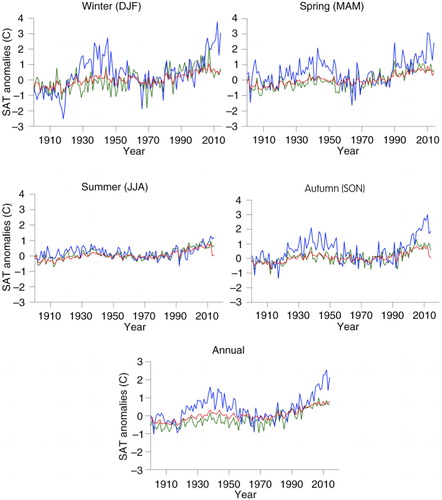
Table 1. Absolute maximum (+) SAT anomalies (C) for year when registered

Latitude	Winter	Spring	Summer	Autumn	Annual
zone	(DJF)	(MAM)	(JJA)	(SON)
40–65°N	2.15; 2007	1.24; 1990	0.96; 2012	1.31; 2005	0.99; 2007
65–90°N	3.76; 2012	3.08; 2010	1.29; 2012	3.01; 2012	2.54; 2012
0–90°N	1.06; 2007	0.75; 2007	0.79; 2012	0.84; 2010	0.72; 2010

Table 2. Seasonal and annual SAT trends (C/100yr) averaged over 1900–2014

Latitude	Winter	Spring	Summer	Autumn	Annual
zone	(DJF)	(MAM)	(JJA)	(SON)
40–65°N	1.17	1.09	0.68	0.70	0.97
65–90°N	1.72	1.02	0.29	0.98	0.99
0–90°N	0.86	0.81	0.59	0.63	0.77

All values are positive (+).

Over the whole period 1900–2014, SAT trends for all latitude zones are largest for winter and smallest for summer (Table 2). The maximum SAT trend (1.72 °C/100 yr) is observed for the Arctic in winter while the minimum trend (0.29 °C/100 yr) occurred in the Arctic in summer. Only in autumn and winter are the maximum SAT trends observed in the Arctic. For other seasons, SAT trends are smallest for the Arctic and largest for mid-latitudes. The annual mean SAT since 1900 was 0.77 °C/100 yr for the NH but larger, ~0.99 °C/100 yr, for mid-latitudes and the Arctic.

However, the overall linear trend on a century scale is neither an ideal measure nor an optimal metric for Arctic amplification, given the strong warming and cooling – which reflect real climate dynamics – on interannual to multidecadal time scales. Therefore, to reveal the time evolution of trends, we calculated successive 30-yr SAT linear trends for the same three latitudes zones (Fig. 2). From 1900–1940, these trends are positive. In winter, spring and autumn, they are larger for the Arctic than for the mid-latitudes and NH. The same is the case for the annual mean. During this period, the absolute values of SAT trends in winter are the largest observed in the 20th century (3.8C/30 yr).

Fig. 2 Seasonal and annual successive 30-yr linear SAT trends for three latitude zones: mid-latitudes (40–65°N); Arctic (65–90°N); and Northern Hemisphere (0–90°N) for four seasons and annual. The 30-yr moving trends are computed at 1-yr increments; the x-axis indicates the middle year of 30-yr period, e.g. 1954 indicates 1940–1969, and so on.

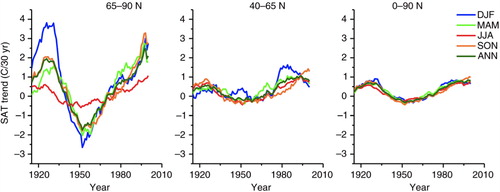
These results differ notably from some previous estimates (e.g. Przybylak, 2007) in the regions where the datasets employ fundamentally different quantities of data for averaging (Kuzmina et al. 2008). Arctic SAT trends are negative, whereas NH and mid-latitudes trends are close to zero. In winter, spring and autumn, absolute values of the Arctic trends are significantly higher than those in NH and mid-latitudes. The largest negative trends occurred in the Arctic in winter in the middle of the 20th century (~−2.7 °C/30 yr). Since the early 1950s, all 30-yr trends in all latitude zones and for all seasons are less negative. In the 1970s they are again positive apart from the SAT trend for the mid-latitudes in spring, which became positive somewhat earlier, in the 1960s. Since the 1980s, the spring and autumn SAT trends for the Arctic have become larger than for the mid-latitudes and NH. In winter, it occurs around 1990. In 1998 SAT trends in the Arctic for winter, spring and autumn reached the value ~3 °C/30 yr. In spring they became the largest over the whole period of observations for this season. Autumn Arctic warming reached the maximum of 3.3 °C/30 yr, exceeding that which took place in the ETCW. In summer there is no significant difference between the Arctic, NH and mid-latitude trends for the whole period of observations.

4. Arctic amplification magnitude

There is no universal metric for assessing Arctic amplification, though a quantitative comparison of temperature changes depending on latitude is implicit. Here for evaluation of Arctic amplification, we define an Arctic Amplification Index (AAI) as the ratio between absolute values of the Arctic and NH trends, calculated in successive 30-yr periods with moving 1-yr intervals. The index is calculated only for the years when both the NH and Arctic trends are significant at the 95 % confidence level – this also prevents a potential arithmetic problem when the denominator (NH trend) approaches zero. This index is different from the index of Bekryaev et al. (2010), who calculated a regression coefficient relating Arctic and global SATs. Bekryaev et al. (2010) state that their regression-based index was developed as a means to alleviate the problem in Polyakov et al. (2002), who used a simple ratio similar to ours. However, the problem with the Polyakov et al. (2002) assessment of ‘no amplification’ appears to be rather in their comparing long-term linear trends rather than the ratios for the warming and cooling events. The same can be mentioned for Chylek et al. (2009) vis-à-vis Chylek et al. (2010), the latter of which focused on comparing long-term trends from the peak of the early warming to the peak of the present warming rather than the actual warming and cooling events, in contrast to Chylek et al. (2009). While the Bekryaev et al. (2010) approach is statistically sound, our AAI is straightforward and effective, especially given our focus on the temporal evolution of warming and cooling and not the long-term trend. However the index values here and those in Bekryaev et al. (2010) are not directly quantitatively comparable, because Bekryaev et al. (2010) used only coastal and land stations while the NansenSAT data also included ocean data (e.g. drifting stations). The temporal evolution of the AAI in each season is shown in Fig. 3.

Fig. 3 Time evolution of the Arctic Amplification Index (AAI) for four seasons. AAI is a ratio between 30-yr linear trends for the Arctic (65–90°N) and Northern Hemisphere (NH) SAT. The index is calculated only for the years when both NH and Arctic trends are significant at the 95 % confidence level. Dotted line indicates AAI = 1, no amplification: Arctic SAT trends are equal to the NH trends. The 30-yr moving AAI is computed at 1-yr increments; the x-axis indicates the middle year of 30-yr period, e.g. 1954 indicates 1940–1969, and so on.

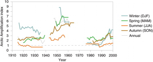
During the ETCW, the values for the AAI > 1 for winter, spring and autumn, indicating the existence of a significant amplification. For winter its magnitude is 3–6, whereas for spring and autumn it is only 1.5–3. During the subsequent cooling period, amplification is observed for all seasons and – in agreement with Chylek et al. (2009) – its magnitude is even higher than for the early warming: AAI varies from 2 to 9, with especially strong amplification found for winter and spring.

The ongoing warming is characterised by substantially smaller magnitude of the Arctic amplification than the previous warming and cooling, with AAI ≤ 4. There is almost no amplification in summer. Spring and autumn amplification is more pronounced, AAI ~1.5–3. There is a tendency for the Arctic amplification strengthening during the last several years for all seasons, especially for winter, which increased from 1–2 to ~4 in the most recent decade. Further, the generally lower AAI values in the recent vis-à-vis the earlier warming should not interpreted as evidence against Arctic amplification – on the contrary, it is evidence for the increasing global warming background upon which amplified Arctic warming is superposed, e.g. Johannessen et al. (2004).

5. Arctic climate regionalisation

In the above analysis and in previous analyses using data aggregated into latitudinal bands (e.g. Polyakov et al., 2002; Chylek et al., 2009; Bekryaev et al. 2010) regional patterns in warming and cooling were not resolved. In different regions of the Arctic, changes in climate conditions depend on the type of atmospheric and oceanic circulation and the nature of the underlying surface (Bengtsson et al., 2004; Johannessen et al., 2004; Kuzmina et al., 2008). Different Arctic regionalisations have been presented in the past, but were based either on subjective qualitative or semi-quantitative analysis (e.g. Treshnikov, 1985; Alekseev and Svyaschennikov, 1991; Przybylak, 2007) or based on dividing the Arctic into uniform longitudinal sectors (Wood and Overland, 2010).

Here we identify natural regions of SAT variability in an objective, statistically-based manner applying hierarchical cluster analysis (Hartigan, 1975) to ERA-40 SAT fields (Uppala et al., 2005). The defined regionalisation is shown in Fig. 4a. The reason that the ERA-40 dataset was used for cluster analysis instead of NansenSAT – which was used in this study for the long-term analysis of SAT variability and trends – is that ERA-40 dataset has no gaps in high northern latitudes. Missing SAT values that occur in NansenSAT, mainly in highest latitudes, obstruct the cluster analysis and lead to the creation of artificial clusters; this takes place even if missing values are substituted by long-term SAT averages. To illustrate this, we also created clusters on the basis of NansenSAT (Fig. 4b). While yielding geographical locations of clusters generally similar to ERA-40, NansenSAT nonetheless originates some artificial clusters, such as evident in the Central Arctic and Siberia. Therefore, the choice of ERA-40 for regionalisation is reasonable. Moreover, a detailed comparison of ERA-40 and NansenSAT data demonstrated good agreement between them in common areas (Kuzmina et al., 2008).

Fig. 4 Maps showing six Arctic regions defined by hierarchical cluster analysis using Annual average SATs from (a) ERA-40 reanalysis and (b) NansenSAT. Long-term mean (c) SAT standard deviation and (d) mean sea-level pressure from ERA-40 data.

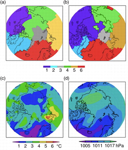
For determining the regional clusters, we used ERA-40 2-m monthly mean SAT over the period 1958–2002, which were annually averaged and applied in the cluster analysis. Because the regional-scale distribution of air temperature corresponds generally with the surface pressure at high latitudes, it suggests that the temperature anomalies are determined by the positions of the quasi-stationary wave pattern of the NH atmospheric circulation (e.g. Bengtsson et al., 2004). Therefore, the regionalisation is considered physically reasonable as it uses long-term temperature means for its creation and provides the opportunity to capture the main features of spatial distribution of the major Arctic climate parameters including circulation patterns. We also note that the boundaries of the defined clusters coincide with the outlines of the continents and climatic position of the sea-ice edge.

After cluster determination, the data coverage of NansenSAT in each cluster was examined. The density of the station network was changing mostly during the first half of the 20th century. Thus, Clusters 3 and 4 were not consistently represented until the 1930s, whereas all other clusters were represented satisfactory during the whole period under consideration. From the 1950s, all clusters are fully covered by SAT data.

There are several distinct natural regions in the Arctic. The main differences between them appear during the cold season due mainly to heat advection via atmospheric circulation. In some regions (e.g. the northern North Atlantic) the warm ocean currents also have a great impact. In summer, climatic differences are smoothed out. As mentioned above, the temperature anomalies at high latitudes are determined by the positions of the quasi-stationary wave pattern of the NH atmospheric circulation. In the Arctic in winter, there is a high-pressure system with the ridges of the Siberian and Canadian Highs, while the Icelandic Low extends in an easterly direction reaching Severnaya Zemlya (Fig. 4d). The spatial distribution of long-term temperature variance (Fig. 4c) corresponds with the location of the main pressure systems. The created regionalisation should capture and reflect these circulation features in a climatic sense.

The results of the cluster analysis indicate six different regions, as depicted in Fig. 4a:

• Cluster 1 covers the North America region. In winter, high-pressure systems developing in the northwest of Canada and northeast Siberia dominate over this region. The temperature in winter reaches −38 °C in the northern part of the region and −25 °C to −30 °C in the southern part.

• Cluster 2 represents Greenland, Baffin Bay and part of the Canadian Archipelago. The Baffin Bay region is situated in the pathway of North Atlantic cyclones, which are especially frequent in winter. This results in higher winter temperatures here than in adjacent areas. The eastern and northern part of this cluster is under the influence of temperate West Greenland Current. Migrating cyclones associated with the Icelandic Low influence the southern part of Greenland. For the northern part of Greenland, the combination of high elevation, the presence of glacial ice and strong radiative cooling at the surface boundary layer creates a meteorological regime dominated by anticyclonic circulation during the year.

• Cluster 3 covers the North Polar area and Arctic Ocean adjacent to the Kara Sea. Climatic conditions retain some of the characteristics of the marine climate, especially near the Atlantic region, where the influence of the cyclones is strong. However the warming effect of the Atlantic waters that sinks to deeper layers of the ocean is not large. Air temperatures are −24 to −26C reaching −32C near the pole, with noticeable horizontal gradients.

• Cluster 4 covers East Siberia and part of the Arctic and North Pacific oceans. In winter, this cluster is under a strong influence of anticyclonic circulation developing over northeastern Siberia and the eastern part of the Arctic Ocean. This region is characterised by low temperatures over both marine and land areas.

• Cluster 5 represents the major portion of West Siberia and the Kara Sea. In this region, the influence of cyclonic circulation is clearly manifested, although in the east part of the Kara Sea, the impact of anticyclonic circulation associated with the Siberian and Arctic high-pressure systems in wintertime is more evident. Further, Novaya Zemlya serves as a barrier to the penetration of warm water from the Barents Sea and cyclones coming from the west. As a result, over the western coast of Novaya Zemlya there are very large horizontal temperature gradients that diminish sharply in the southern part of the Kara Sea.

• Finally, Cluster 6 covers northern Europe, the Barents and Nordic Seas and the northern North Atlantic region. During the cold season, the northern North Atlantic is under a very strong influence of cyclonic circulation, also strongly influenced by the warm ocean currents extending from the Gulf Stream. Heat transport resulting from atmosphere and ocean circulation thus creates exceptionally high winter temperatures in the region.

6. Arctic regional SAT analysis

The cluster definition in Section 5 was based on ERA-40 SAT fields; however, the further analysis of the Arctic regional SAT variability and trends was performed using the century-scale NansenSAT data set. SAT variability and trends over the past century were estimated for each Arctic region/cluster (Fig. 5a). Positive 100-yr trends were found for all clusters, significant at the 95 % confidence level for Clusters 1, 3, 4 and 5. Relatively large variability occurs in Clusters 1 and 3. Generally, the changes in the clusters adjacent to the Pacific Ocean and Central Arctic are larger (Clusters 1, 3 and 4). The lowest variability and trends are found in the northern Europe, Nordic Seas, northern North Atlantic and Greenland (Clusters 2 and 6).

Fig. 5 (a) Annual SAT anomalies 1900–2014 and their linear trends for each cluster; (b) 30-yr moving trends in annual SAT; (c) ratio between 30-yr moving trends in annual SAT for each cluster and the entire Arctic region. In (b) and (c), the x-axis indicates the middle year of 30-yr trends, e.g. 1954 indicates 1940–1969, and so on. For the clusters where the data coverage is less than 50 %, SAT anomalies and trends are shown with dotted lines.

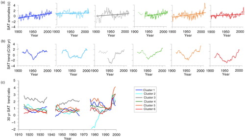
The two major warming periods are found in all clusters. The ETCW was most intensive in the North Pole area and Arctic Ocean adjacent to the Kara Sea; the maximum SAT anomaly reached there was approximately +3C in 1938. The ongoing warming is pronounced in the Central Arctic, Siberia and North America (Clusters 1, 3, 4 and 6). Maximum SAT anomaly, observed in 1998 over North America, was +2.6 C. The ETCW in the Arctic has recently been exceeded by the ongoing warming in Clusters 1, 4 and 5.

Figure 5b shows annual 30-yr successive SAT trends for the different clusters. The temporal evolution of these trends indicates the warming and cooling periods more clearly than SAT anomalies in Fig. 5a. We used these 30-yr successive SAT trends for assessing the contributions of different Arctic regions to the amplification. For this we calculated the ratio between 30-yr SAT trends for each cluster and the entire Arctic (Fig. 5c). During the ETCW and subsequent cooling period, the largest contribution to temperature changes (increase and decrease, respectively) is provided by the Cluster 3 (the North Pole area and Arctic Ocean adjacent to the Kara Sea). A smaller contribution to the Arctic amplification is provided also by Cluster 2 during the ETCW and by Cluster 5 during the subsequent cooling. All other clusters are characterised by approximately the same values of SAT trend as the whole Arctic or even less; the latter fact means that these regions partially offset the Arctic amplification. During the recent warming period, the largest contribution to temperature increase is provided by Clusters 1 and 5 (North America and West Siberia/Kara Sea, respectively). Cluster 4 also gives a small contribution to amplification. Clusters 2, 3 and 6 exhibit reduced amplification, especially Cluster 2 (Greenland, Baffin Sea and part of the Canadian Archipelago) where observed SAT trend is negative and opposite to the whole Arctic trend during 1975–1985.

Analysis of seasonal trends for the different clusters is shown in Fig. 6. The summer trends for all clusters are small; there is no significant difference between SAT trends for different regions. The largest SAT trends (both positive and negative) are observed in Cluster 3 (North Pole area and Arctic Ocean adjacent to the Kara Sea) for all seasons except summer. Thus, during the first half of the 20th century they accounted for approximately +8C/30 yr in winter, +3C/30 yr in spring and +5C/30 yr in autumn. In the mid-century, SAT trends there reached approximately −6C/30 yr in winter and −3C/30 yr in spring and autumn.

Fig. 6 Thirty-years moving trends as in Fig. 5b, but seasonally: (a) winter (DJF), (b) spring (MAM), (c) summer (JJA) and (d) autumn (SON).

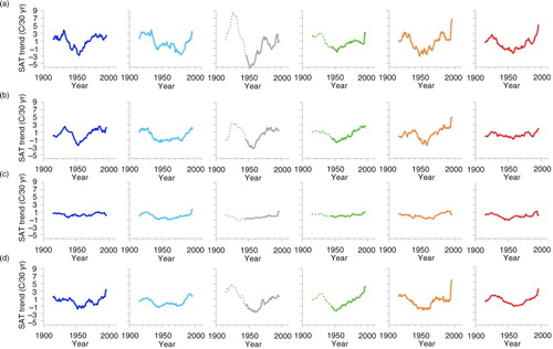
In contrast, the winter, spring and autumn SAT trends have increased in essentially all clusters since the 1950s. The only exception is Cluster 2 (Greenland, Baffin Bay and part of the Canadian Archipelago) where the winter SAT trend continued to decrease and reached most negative value in about 1980 accounted for −2.6C/30 yr; this appears to reflect the strong upward trend in the North Atlantic Oscillation (NAO), which induces northerly wind and negative temperature anomalies in the region.

7. Arctic regional SAT and modes of variability

In order to gain insight into the differences in SAT trends in the various regions, here we quantitatively compare them with known large-scale modes of variability in the climate system. Before performing a correlation analysis, we first extracted the long-term secular warming from averaged SAT and each of the climate index time series using Singular Spectrum Analysis (SSA) method (Golyndina et al., 2001). This method combines advantages of other methods, such as Fourier and regression analyses. The result of the SSA processing is a decomposition of the time series into several components, which can often be identified as trends, and other oscillatory series, or noise components.

The time series of residuals for the whole Arctic and for each cluster were then correlated with climate indices based on SLP and sea-surface temperature (SST). The atmospheric circulation index is the station-based NAO index (Jones et al., 1997). [The Arctic Oscillation (AO)/Northern Annular Mode (NAM) indices were also analysed, but because the results were nearly identical to those for the NAO, we present results only for the NAO]. The SST-based indices are the Atlantic Multidecadal Oscillation (AMO) (Enfield et al., 2001) and the Pacific Decadal Oscillation (PDO) (Mantua et al., 1997). Figure 7 shows the running 30-yr annual correlation of SAT time series with PDO, AMO and NAO indices for the whole Arctic and six Arctic regions determined by the cluster analysis.

Fig. 7 Running 30-yr correlation between annual SAT and annual climate indices. The indices are the Pacific Decadal Oscillation (PDO), Atlantic Multidecadal Oscillation (AMO), and North Atlantic Oscillation (NAO). Only correlations greater than|0.3|which are significant at the 95 % confidence level (α<0.05) are shown. (a) Running 30-yr correlation between annual SAT averaged over the region 65–90°N and annual climate indices; (b) running 30-yr correlation between annual SAT and annual climate indices for six Arctic regions (1–6); the x-axis indicates the middle year of 30-yr trends, e.g. 1954 indicates 1940–1969, and so on.

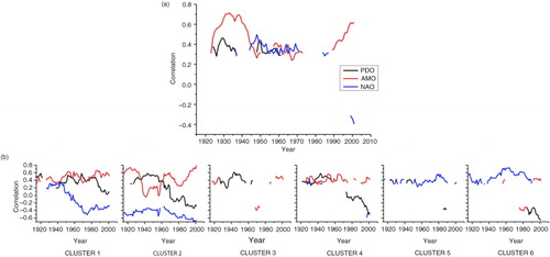
The results of the correlation analysis for the Arctic (Fig. 7a) show that the annual climate indices have the ability to partly predict annual SAT. The most consistently strong linkages are found between the AMO and SAT. The AMO–SAT correlations are uniformly positive for both warming periods. There are several other interesting features that emerge from the correlation analysis for the various indices, regions and periods (Fig. 7b). The indices other than the AMO, while significantly correlated with SAT in many cases, have a much more variable relationship with SAT in the various regions and periods. During both warming periods of 1910–1939 and 1970–2006 (and ongoing), SAT is significantly positively correlated with SST-based indices (AMO and PDO), although the correlation with PDO index was relatively small and did not exceed 0.45 for all clusters. The highest positive correlation was found with the AMO index during the first warming period for Cluster 2 (r=0.7) and during the ongoing warming for Clusters 1 and 2 (r≥0.8). The NAO atmospheric circulation index has both positive and negative correlations, depending on period and region. The highest negative correlation between SAT and the NAO index (∣ r ∣ ≥ 0.7) was found for the Clusters 1 and 2. For the Cluster 2 (Greenland and part of the Canadian Archipelago), the correlation with NAO/AO index was r ≈ − 0.55 during both warming periods.

During the cooling period (1940–1969), the correlation with the PDO index was r ≈ 0.6 for Clusters 1, 2, 3 and 4. The correlation with the AMO index was significant r ≈0.5 only for Cluster 1. The NAO also contributed to the cooling, having a significant correlation with Siberian SAT (Clusters 5 and 6, r ≈ 0.5–0.6).

Comparison of SAT correlations for the two warming periods reveals that during the recent warming, their patterns shifted as follows:

• North American region (Cluster 1): The relationship between AMO index and regional SAT became stronger.

• Greenland and Canadian Archipelago region and part of the Arctic Ocean (Clusters 2 and 3): The strength of the positive correlations with AMO index (r~0.7) reached the ETCW level only for the period 1980–2010.

• Siberian regions (Clusters 5 and 6): The correlation between SAT and the NAO index became insignificant or even negative during the last decades in contrast to positive correlation values during ETCW (r≤0.56).

These results demonstrate that Arctic SAT changes are caused by the combination of different factors. During the first half of the 20th century, greater warming occurred over the pole and some ocean areas (Cluster 3), which was strongly connected with variations of Atlantic SST. These SST anomalies are associated with a hemispheric wavenumber-1 SLP structure in the atmosphere that is amplified through atmosphere–ocean interactions in the North Pacific (Wood et al., 2010). This is consistent with the finding that the modes of variability other than the NAO must be invoked to explain Arctic SAT variability such as observed in the ETCW (Semenov and Bengtsson, 2003). The statistical mode of variability found by Semenov and Bengtsson (2003) to explain the ETCW was not associated with any known atmospheric circulation pattern; subsequently it has been seen to be associated with SST variability and meridional mode of atmospheric circulation that has reappeared in the strong warming of the early 2000s (Overland and Wang, 2005; Overland et al., 2008; Wood et al., 2010).

8. Summary and conclusions

The statistical analysis of SAT variability and trends performed here clearly supports Arctic amplification as a robust, persistent feature of the climate system, a conclusion based on analysis of warming and cooling periods found in the century-scale temperature record. A new AAI has been defined as the ratio between the absolute values of the Arctic and NH trends based on successive 30-yr periods. Analysis of the temporal evolution of the amplification reveals substantial variability depending on the period, season and region. The amplification is stronger during the early 20th century warming (ETCW) than that for the recent years because of the increased global warming background upon which amplified Arctic warming is superimposed.

A new Arctic regionalisation has been calculated based on objective, statistically hierarchical cluster analysis. Six clusters have been defined representing distinct natural regions reflecting atmospheric and ice–ocean dynamics. Each of the regions has different SAT variability trend characteristics and thereby different contributions to the observed Arctic amplification.

Statistical analysis of correlations between the AMO, NAO and PDO modes of variability and SAT for the different clusters and Arctic as a whole supports the concept that Arctic SAT variability is modulated primarily by SST variability on similar time scales, with the North Atlantic region being of central importance. As found here, North Atlantic multidecadal variability such as that characterised by the AMO index is significantly and consistently correlated with Arctic warming and cooling, most strongly during warming periods. However, the linkages between SAT and the AMO and other climate indices have significant regional and seasonal variability. This suggests a conceptual model for future Arctic warming that will be composed of a complex pattern of amplified greenhouse gas (GHG) warming superposed with AMO-related variability – which affects Northern Hemisphere SAT (Wu et al., 2015) as well as the Arctic – and regional modes of variability on both comparable and shorter time scales.

9. Acknowledgements

This research was carried out with the following support: The Research Council of Norway (RCN) ARCWARM project (‘Arctic and sub-Arctic climate system and ecological response to the early 20th century warming’) and the RCN joint Norwegian–Russian project NORRUS, both with OMJ as project leader; The EU FP7 project EuRuCAS (‘European–Russian Centre for cooperation in the Arctic and Sub-Arctic environmental and climate research’) Grant Agreement no. 295068; and the Russian Foundation for Basic Research (RFBR) project ‘Climate variability and change in the Eurasian Arctic during the 21st century’, no. 12-05-93092 with LPB as project leader. We are grateful to the editor and anonymous reviewer, who helped us to improve the quality of our manuscript.

References

- Alekseev G. V. , Svyaschennikov P. N . Natural variability of climate characteristics in Northern Polar Region and Northern Hemisphere. 1991; St. Petersburg, Russia: Gidrometeoizdat. 159. (in Russian).
- Arctic Climate Impact Assessment (ACIA). 2005; Cambridge, UK: Cambridge University Press. 1042.
- Arrhenius S . On the influence of carbonic acid in the air upon the temperature of the ground. Philos. Mag. J. Sci. 1896; 5: 237–276.
- Bekryaev R. V., Polyakov I. V., Alexeev V. A. Role of polar amplification in long-term surface air temperature variations and modern Arctic warming. J. Clim. 2010; 23: 3888–3906. DOI: http://dx.doi.org/10.1175/2010JCLI3297.1.
- Bengtsson L. , Semenov V. , Johannessen O. M . The early twentieth-century warming in the Arctic – a possible mechanism. J. Clim. 2004; 17: 4045–4057.
- Brohan P., Kennedy J. J., Harris I., Tett S. F. B., Jones P. D. Uncertainty estimates in regional and global observed temperature changes: a new data set from 1850. J. Geophys. Res. 2006; 111: 12106. DOI: http://dx.doi.org/10.1029/2005JD006548.
- Chylek P., Folland C. K., Lesins G., Dubey M. K., Wang M.-Y. Arctic air temperature change amplification and the Atlantic multidecadal oscillation. Geophys. Res. Lett. 2009; 36: 14801. DOI: http://dx.doi.org/10.1029/2009GL038777.
- Chylek P. , Folland C. K . Arctic climate sensitivity: Anthropogenic warming and multi-decadal variability. Eos Trans. AGU. 2010; 91(26): Meet. Am. Suppl., Abstract A32B-02.
- Dee D. P. , Uppala S. M. , Simmons A. J. , Berrisford P. , Poli P. , co-authors . The ERA-Interim reanalysis: configuration and performance of the data assimilation system. Quart. J. R. Meteorol. Soc. 2011; 137: 553–597.
- Enfield D. B. , Mestas-Nunez A. M. , Trimble P. J . The Atlantic multidecadal oscillation and its relationship to rainfall and river flows in the continental U.S. Geophys. Res. Lett. 2001; 28: 2077–2080.
- Golyndina N. , Nekrutkim V. , Zhiglyavsky A . Analysis of time series structure. SSA and related techniques. 2001; New York, USA: Chapman & Hall/CRC Press. 320.
- Hartigan J. A . Clustering Algorithms. 1975; John Wiley & Sons, New York.
- Hwang T., Frierson D. M. W., Kay J. E. Coupling between Arctic feedbacks and changes in poleward energy transport. Geophys. Res. Lett. 2011; 38: 17704. DOI: http://dx.doi.org/10.1029/2011GL048546.
- Intergovernmental Panel on Climate Change (IPCC). Climate change 2013: the physical science basis. Contribution of Working Group I to the Fifth Assessment Report of the Intergovernmental Panel on Climate Change. 2013; Cambridge, United Kingdom: Cambridge University Press. 1535. (eds. T. F. Stocker, D. Qin, G.-K. Plattner, M. Tignor, S. K. Allen, and co-authors.
- Johannessen O. M. , Bengtsson L. , Miles M. W. , Kuzmina S. I. , Semenov V. A. , co-authors . Arctic climate change: observed and modelled temperature and sea ice variability. Tellus A. 2004; 56: 328–341.
- Jones P. D. , Jónsson T. , Wheeler D . Extension to the North Atlantic oscillation using early instrumental pressure observations from Gibraltar and south-west Iceland. Int. J. Climatol. 1997; 17: 1433–1450.
- Jones P. D. , New M. , Parker D. E. , Martin S. , Rigor I. G . Surface air temperature and its variations over the last 150 years. Rev. Geophys. 1999; 37: 173–199.
- Kahl J. D. , Charlevoix D. J. , Zaitseva N. A. , Schnell R. C. , Serreze M. C . Absence of evidence for greenhouse warming over the Arctic Ocean in the past 40 years. Nature. 1993; 361: 335–337.
- Kuzmina S. , Johannessen O. M. , Bengtsson L. , Aniskina O. , Bobylev L . High northern latitude surface air temperature: comparison of existing data and creation of a new gridded data set 1900–2000. Tellus A. 2008; 60: 289–304.
- Mahajan S. , Zhang R. , Delworth T. L . Impact of the Atlantic Meridional Overturning Circulation (AMOC) on arctic surface air temperature and sea ice variability. J. Clim. 2011; 24: 6573–6581.
- Manabe S. , Stouffer R. J . Sensitivity of a global climate model to an increase of CO2 concentration in the atmosphere. J. Geophys. Res. 1980; 85: 5529–5554.
- Mantua N. J. , Hare S. R. , Zhang Y. , Wallace J. M. , Francis R. C . A Pacific interdecadal climate oscillation with impacts on salmon production. Bull . Am. Meteor. Soc. 1997; 78: 1069–1079.
- Overland J. E., Wang M. The third Arctic climate pattern: 1930s and early 2000s. Geophys. Res. Lett. 2005; 32: 23808. DOI: http://dx.doi.org/10.1029/2005GL024254.
- Overland J. E. , Wang M. , Salo S . The recent Arctic warm period. Tellus A. 2008; 60: 589–597.
- Polyakov I. V., Alekseev G., Bekryaev R., Colony R. L., Bhatt U. S., co-authors. Observationally based assessment of polar amplification of global warming. Geophys. Res. Lett. 2002; 29: 1878. DOI: http://dx.doi.org/1029/2001GL011111.
- Przybylak R . Recent air-temperature changes in the Arctic. Ann. Glac. 2007; 46: 316–324.
- Rigor I. G. , Colony R. L. , Martin S . Variations in surface air temperature observations in the Arctic, 1979–97. J. Clim. 2000; 13: 896–914.
- Screen J. A. , Simmonds I . The central role of diminishing sea ice in recent Arctic temperature amplification. Nature. 2010; 464: 1334–1337.
- Semenov V. A. , Bengtsson L . Modes of the wintertime Arctic temperature variability. Geophys. Res. Lett. 2003; 30: 1781–84.
- Serreze M. C. , Barrett A. P. , Stroeve J. C. , Kindig D. N. , Holland M. M . The emergence of surface-based Arctic amplification. Cryosphere. 2009; 3: 11–19.
- Serreze M. C. , Barry R. G . Processes and impacts of Arctic amplification: a research synthesis. Glob. Planet. Change. 2011; 77: 85–96.
- Thompson D. W. J., Wallace J. M., Kennedy J. J., Jones P. D. An abrupt drop in Northern Hemisphere sea surface temperature around 1970. Nature. 2011; 467 444–447. DOI: http://dx.doi.org/10.1038/nature09394.
- Treshnikov A. F . Atlas Arctiki. 1985. (Arctic Atlas). Main Administration of Geodesy and Cartography under the Council of Ministers of the USSR, Moscow (in Russian).
- Uppala S. M. , Kållberg P. W. , Simmons A. J. , Andrae U. , da Costa Bechtold V. , co-authors . The ERA-40 re-analysis. Quart. J. Royal. Meteorol. Soc. 2005; 131: 2961–3012.
- Wang X. , Key J. R . Arctic surface, cloud, and radiation properties based on the AVHRR Polar Pathfinder Data Set. Part II: recent trends. J. Clim. 2005; 18: 2575–2593.
- Wood K. R. , Overland J. E . Early 20th century Arctic warming in retrospect. Int. J. Climatol. 2010; 30: 1269–1279.
- Wood K. R., Overland J. E., Jonsson T., Smoliak B. V. Air temperature variations on the Atlantic-Arctic boundary since 1802. Geophys. Res. Lett. 2010; 37: 17708. DOI: http://dx.doi.org/10.1029/2010GL044176.
- Wu Y., Latif M., Park W. Multiyear predictability of Northern Hemisphere surface air temperature in the Kiel Climate Model. Clim. Dynam. 2015; 46: 1–12. DOI: http://dx.doi.org/10.1007/s00382-015-2871-z.