Demonstrating the value of larger ensembles in forecasting physical systems

Abstract

Ensemble simulation propagates a collection of initial states forward in time in a Monte Carlo fashion. Depending on the fidelity of the model and the properties of the initial ensemble, the goal of ensemble simulation can range from merely quantifying variations in the sensitivity of the model all the way to providing actionable probability forecasts of the future. Whatever the goal is, success depends on the properties of the ensemble, and there is a longstanding discussion in meteorology as to the size of initial condition ensemble most appropriate for Numerical Weather Prediction. In terms of resource allocation: how is one to divide finite computing resources between model complexity, ensemble size, data assimilation and other components of the forecast system. One wishes to avoid undersampling information available from the model's dynamics, yet one also wishes to use the highest fidelity model available. Arguably, a higher fidelity model can better exploit a larger ensemble; nevertheless it is often suggested that a relatively small ensemble, say ~16 members, is sufficient and that larger ensembles are not an effective investment of resources. This claim is shown to be dubious when the goal is probabilistic forecasting, even in settings where the forecast model is informative but imperfect. Probability forecasts for a ‘simple’ physical system are evaluated at different lead times; ensembles of up to 256 members are considered. The pure density estimation context (where ensemble members are drawn from the same underlying distribution as the target) differs from the forecasting context, where one is given a high fidelity (but imperfect) model. In the forecasting context, the information provided by additional members depends also on the fidelity of the model, the ensemble formation scheme (data assimilation), the ensemble interpretation and the nature of the observational noise. The effect of increasing the ensemble size is quantified by its relative information content (in bits) using a proper skill score. Doubling the ensemble size is demonstrated to yield a non-trivial increase in the information content (forecast skill) for an ensemble with well over 16 members; this result stands in forecasting a mathematical system and a physical system. Indeed, even at the largest ensemble sizes considered (128 and 256), there are lead times where the forecast information is still increasing with ensemble size. Ultimately, model error will limit the value of ever larger ensembles. No support is found, however, for limiting design studies to the sizes commonly found in seasonal and climate studies. It is suggested that ensemble size be considered more explicitly in future design studies of forecast systems on all time scales.

• chaotic systems
• data assimilation
• ensemble forecasting
• forecast value
• predictability
• probabilistic forecasting
• scoring rule
• probability

1. Introduction

Probability forecasting of non-linear physical systems is often achieved via a Monte Carlo approach: an ensemble of initial conditions is propagated forward in time (Lorenz, 1969; Palmer et al., 1992; Toth and Kalnay, 1993; Leutbecher and Palmer, 2008) and this ensemble might then be interpreted as a probability distribution (Brocker and Smith, 2008). Many open questions remain regarding relatively basic issues of ensemble design given fixed, finite computational resources. It is argued that increasing the ensemble size well beyond 8 or 16 members can significantly increase the information in a probability forecast. This is illustrated both in chaotic mathematical systems (where the ‘model’ is perfect) and a related physical system (an electronic circuit) where the mathematical structure of the model is imperfect. Information in the forecast is quantified by I.J. Good's logarithmic skill score (Good, 1952) (hereafter called ignorance or IGN), and interpreted both in terms of bits of information and in perhaps more familiar terms of improved return on investment. In general, using larger ensembles increases the information in the forecast, even for the largest ensembles considered (contrasting 128 members with 256). The details, however, are shown to vary with the lead time evaluated, the fidelity of the model and the data assimilation scheme. The major conclusion of this article is that the experimental design of future ensemble forecast systems should incorporate a more systematic evaluation of the utility of larger ensembles.

The utility of ensemble forecasts in meteorology was noted by Leith (1974), who showed that increasing the ensemble size resulted in superior forecasts. In economics, the work of Bates and Granger (1969) was revolutionary in making a case for ensemble forecasts, arguing that ensemble forecasts are superior to single forecasts as noted by Leith (1974), however, ensembles were interpreted merely to obtain better point forecasts; Leith (1974) found an eight-member ensemble to be near optimal in minimising the root mean square error of the ensemble mean.

Tennekes (1988) urged weather forecasting centres around the world to issue quantitative predictions of the skill of each individual forecast. If one considered the ensemble mean as a point forecast, for instance, the ensemble spread might provide a measure of uncertainty in as much as it reflects the local sensitivity of the model to uncertainty in the initial condition. Point-forecasting via the ensemble mean is ill-advised, however, when there is useful information in the distribution that would be lost. And when interpreting the ensemble as a probability distribution, the insights of Leith (1974) and Ferro et al. (2012) regarding the ensemble mean as a point forecast simply do not apply. The key point here is that selecting an ensemble size for probabilistic forecasting is a different goal from optimising the root-mean-square error of the ensemble mean.

Richardson (2001) addressed the question of ensemble size in the case of categorical forecasts (where probabilities are placed on a set of discrete, mutually exclusive events), assuming that each ensemble is drawn from the same distribution as its outcome. Using the Brier score (Brier, 1950), reliability diagrams and the cost–loss ratio, he concluded that the appropriate ensemble size varies with the user. The Brier score lacks a general interpretation [its interpretation as an (limited) approximation to the ignorance score is revealed in Todter and Ahrens (2012)], and the assumption that the ensemble members are drawn from the same distribution as the outcome is unrealistic in practice. Furthermore, the discussion focuses on binary events, rather than a forecasting scenario with continuous variables. Ferro et al. (2008) reviewed several papers that discuss the effect of ensemble size on the Brier score, ranked probability score and the continuous ranked probability score, but questions of ensemble size were left open. Muller et al. (2005) proposed a modified version of the ranked probability score that would not be biased when ensembles are small, without tackling the question of how large an ensemble should be. Considering the ECMWF ensemble prediction system, Buizza and Palmer (1998) studied the effect of increasing ensemble size up to 32 members using the root-mean-square error, spread-skill relation, receiver operating characteristic (ROC) statistic, Brier score and ranked probability score. The probabilistic evaluation therein was restricted to categorical events interpreted using a simple count of model simulations. Simple ‘bin and count’ schemes to obtain forecast probabilities are inferior to interpreting the ensemble as a continuous distribution (Silverman, 1986).

Despite the foregoing efforts, the question of just how large an ensemble should be remains a burning issue in the meteorological community and a topic of sometimes heated discussion. This article revisits this longstanding question and suggests that the argument for small ensemble size in probability forecasting has neither analytic support nor empirical support; it considers ensemble size as a problem in probability density forecasting and highlights the benefits of a high fidelity (but imperfect) model and a good ensemble formation scheme (i.e. good data assimilation). Density forecasting requires interpreting a set of ensemble members as a probability density function (Brocker and Smith, 2008). Users who are interested in probabilities of specific events such as threshold exceedance can of course use density forecasts to estimate the probabilities of such events. For a given ensemble size, such estimates are expected to be superior to those obtained by a simple count (Silverman, 1986). The following section presents tools for assessing the skill of forecasts. It is followed by a treatment of density estimation when each ensemble member and the outcome are drawn from the same distribution. The choice of ensemble size for probability forecasting, both for imperfect models of mathematical systems and a physical system, is then considered in Sections 4 and 5. While the focus of this article is forecast skill, Section 6 provides a discussion of other properties of forecast distributions. Section 7 contains discussion with the take-home message being that the enduring focus on smaller ensembles should be put under increased scrutiny.

2. Quantifying the skill of a forecast system

The skill of forecast distributions can be contrasted within an investment framework by quantifying the improvement (or degradation) in the rate of return of an investment strategy using those forecast systems. Such a framework, which is equivalent to traditional betting scenarios (Kelly, 1956), is presented in this section. The focus here is on the information content of the forecast distribution, which directly reflects its operational value, as discussed in this section.

Probability distributions have many properties in addition to their skill as forecasts. Notions of reliability [the extent to which observed relative frequencies match forecast probabilities (Brocker and Smith, 2007)], sharpness [a measure of how concentrated distributions are independent of their skill (Gneiting et al., 2007)] and resolution [the ability of a forecasting system to resolve events with different frequency distributions (Brocker, 2015)], each reflect aspects of the forecast distribution or of the forecast–outcome archive. Observations based on these properties are given in Section 6; additional details can be found in Appendix B. The focus of this article, however, falls on the skill (information content) of a probability forecast system regarding a target outcome, not one of the myriad of properties held by the probability distributions per se.

2.1. An investment framework

Consider two competing investors. Each investor uses a forecast system based upon the same simulation model, but the two systems use ensembles of different sizes. The quantity of interest is then the expected growth rate of the wealth of one system (the investor) given odds from the other system (the bookmaker). If this rate is positive, then the investor's wealth will grow whilst it will fall if the rate is negative. The expected rate of growth of the investor's wealth is reflected in the effective interest rate. The symmetry properties of this measure are attractive: changing the roles of the investor and bookmaker does not alter the results. The use of effective interest rate to communicate the value of probabilistic forecasts in meteorology was proposed by Hagedorn and Smith (2009); as illustrated in this section it reflects a proper skill score. The continuous case is considered after first introducing the betting strategy in the categorical case (Kelly, 1956).

2.1.1. The categorical case.

Consider an investor with a forecast probability distribution on a set of mutually exclusive events such that1

Given initial capital c₀ to invest, consider the bookmaker to offer odds according to his or her probability distribution (not necessarily true probabilities of the events), where . The bookmaker issues the odds¹ o _i =1/q _i . The investor places a stake s _i on category i such that , this is the fully invested case: he or she invests all the wealth during each round. In this case, the strategy that maximises his or her expected rate of growth of wealth is to set (Kelly, 1956)2

Kelly argued that, given belief in a probability distribution, wealth should be distributed according to that probability distribution. Think of what could happen if the investor placed all his wealth only in those categories that posted high odds. If none of those categories materialised, his wealth would become zero. For similar reasons it is ill-advised to place bets only on those categories for which p _i >q _i in this ‘fully invested’ scheme [both Hagedorn and Smith (2009) and Kelly (1956) discuss other schemes as well]. Based on the stake placed according to eq. (2), the investor will receive a payoff c₁=s _i o _i , when the ith category materialises. This can be rewritten as3

The investor's wealth will either grow or shrink by a factor r=p _i /q _i according to whether p _i >q _i or p _i <q _i . Call the factor r the return ratio.

Given two competing forecast systems, p _t =(p_1t ,…,p _Nt ) and q _t =(q_1t ,…,q _Nt ) at time t, the return ratio corresponding to the outcome falling in the bin is , where i _t ∈ {1,…,M}. Note that r _t is not indexed by i _t for notational economy since i _t is a random variable that depends on t as well. If the game is played repeatedly, then after time T 4

At a given instant, the wealth will either grow or shrink according to whether r _t >1 or r _t <1, respectively. The geometric average of our returns is given by5

which gives the average factor by which the wealth grows from one time step to another. The effective interest rate, Υ _T , for this investment is defined as6

Taking base two logarithms (to obtain results in bits) of eq. (5) yields7

where i _t ∈ {1,…,M}, and is the average ignorance score proposed by Good (1952).

The relative ignorance of forecast distributions to forecast distributions is then defined by〈IGN〉 _{p , q=} 〈IGN〉 _p –〈IGN〉 _q . From eq. (7), one obtains , after taking exponentials on both sides. Upon substituting this term into eq. (6) one obtains8

Define competitive advantage to be the improvement in the effective interest rate, in percent, that using one forecast system achieves against another forecast system; for example, the competitive advantage of a forecast system using the same simulation model but with a larger ensemble size is considered in this paper. Equation (8) shows the simple relationship between relative ignorance and the effective interest rate. Thus the effective interest rate reflects a proper skill score; discussion of the competitive advantage gained (rather than bits of information added) can sometimes ease communication of forecast value.

2.1.2. The continuous case.

Binning continuous target variables and then evaluating the resulting categorical forecasts runs the risk of loss both of generality and of robustness, as the relevance of the results may depend on the particular categories, binning method, and so on. Furthermore, ensemble members need not be interpreted as reflecting actual probabilities directly; estimating probabilities by counting the fraction of members that fall into a particular category is ill-advised, due to the effects of model error, finite ensemble size and the quality of data assimilation, amongst other reasons. This argues for interpreting the ensembles as probability densities. The ignorance score is used to estimate free parameters in the ensemble interpretation; this is described in detail in the next section. All forecast evaluations in this article are out of sample. Given that two competing forecast systems have densities f _t (x) and g _t (x), the probability of the ith bin can be obtained as and , where i=1,…,M. Using a first-order approximation as max{∣x _i −x _i-1∣}→0, yields the return for the investor at time t as r _t =f _t (ξ _t )/g _t (ξ _t ), where ξ _t is the outcome at time t. Parameters which minimise the ignorance score (out of sample) will maximise the growth rate of an investor's stake; this holds for the house as well. In competition, it is the relative skill of the two forecast systems that determines which ‘growth rate’ is positive and which is negative.

3. Density estimation

In this section, the quality of distributions for different ensemble sizes is considered purely in the context of estimating the distribution from which the ensemble members were drawn. In this case kernel density estimation (Silverman, 1986) is appropriate. Alternatively when the outcome is not drawn from the same distribution as the ensemble members, kernel dressing (Brocker and Smith, 2008) is used (see Section 4). In this section, only the normal distribution and a mixture of normals are considered. The value of increasing the ensemble size is quantified via the competitive advantage introduced in Section 2.1.

The standard normal is:9

The Gaussian mixture considered is10

where11

with μ₁=2 and μ₂=−2. The mean of this mixture distribution is μ=−2/3 and its variance is σ ²=41/9. One can also consider the effect of ensemble size on the estimation of the normal distribution of mean μ and variance σ ², which is equal to those of the foregoing mixture distribution.

In order to mimic the scenario in forecasting, consider drawing D distinct n-member ensembles. This n is called the ensemble size. Statistically insightful evaluations of forecasting performance will assess performance over forecast–outcome pairs. Consider the set of D ensembles to be , where each member of the set constitutes an ensemble drawn from some underlying distributions (either the normal distribution or the mixture). For each ensemble, estimate the underlying density using a sum of kernels via (Parzen, 1962; Silverman, 1986)12

where Gaussian kernels with kernel width σ _n >0 are employed. In this case the kernel width is taken to be uniform over all ensembles of a given size n. For each X ^(d,n), an outcome Y ^(d) is randomly selected from the underlying distribution. The ignorance score is13

In the forecast systems in subsequent discussions, the kernel width was selected by minimising the ignorance score (the results presented are out of sample). In the subsequent calculations, set D=512 and the ensemble size n ∈ {1,2,…,128}. The variance of the distribution given by eq. (12) is14

where μ _d is the ensemble mean.

The graphs in Fig. 1 correspond to the standard normal distribution (purple line) and the mixture distribution (blue dashed line). For a given distribution, the kernel width is chosen separately for each ensemble size to minimise IGN [see eq. (13)].

Fig. 1 Simple Gaussian and mixture distributions. Top left: Graph of competitive advantage when the ensemble size is doubled as a function of the final ensemble size (shown on the horizontal axis). That is, this is the IGN of an ensemble relative to an ensemble half its size. Top right: Change in IGN when the ensemble size is doubled as a function of the final ensemble size. Note the inverse relationship between competitive advantage and relative ignorance. Bottom left: Graph of kernel width versus ensemble size. Bottom right: Graphs of the reliability _PIT as a function of ensemble size. The underlying distributions are the standard normal (solid purple) and a mixture (blue dashed) of normals, π(x), given in eq. (10). For each distribution, at a given ensemble size, the kernel width was chosen to minimise IGN. The bars on the left graphs are the 95 % bootstrap re-sampling intervals. Note that the smallest value of the ensemble size in the above graphs is n=1 (a so-called singleton ensemble).

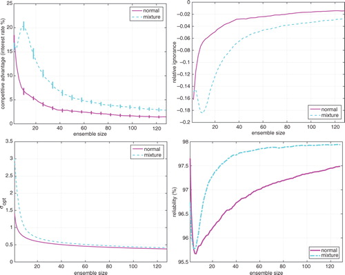
Note that eq. (13) evaluates continuous probability density functions (PDFs) whilst the discussion near eq. (7) considers discrete probabilities. In each case, the forecast system with lower IGN will (in expectation) yield better investment returns. The top left graphs show the competitive advantage gained over a forecaster using ensemble half the size. The top right panel of Fig. 1 presents corresponding graphs of IGN, the logarithmic scoring rule; note that the competitive advantage mirrors the ignorance score. Considering graphs of competitive advantage, it is evident that doubling the ensemble size results in a competitive advantage of at least 1 % (2 %) when the underlying distributions are normal (bimodal). Notice also that, except at the smallest ensemble sizes, the competitive advantage is always greater for the mixture distribution than it is for the normal distributions. Intuitively, one expects a larger ensemble size to capture a bimodal distribution than a unimodal one. To assess this, a normal distribution is compared with a mixture distribution of equal mean and variance. Bimodality of the mixture distribution plays a central role in the increased competitive advantage when the ensemble size is doubled. Distributions with additional fine structure are expected to benefit more, in terms of competitive advantage, when the ensemble size is doubled. This point is revisited in the discussion of probabilistic forecasting in the next section. The lower panels of Fig. 1 present the kernel width at which ignorance is minimised and the reliability _PIT for each of the two distributions as a function of ensemble size; these properties are discussed in Section 6.

4. Probabilistic forecasting

In this section the effect of increasing the ensemble size is considered in a forecasting context with measurement error (i.e. observational noise). In the perfect model scenario (PMS), two cases are considered. In the first case one forecasts from random perturbations of the initial conditions; this ensemble formation scheme will be called inverse observational noise (IN). In the second case, the initial ensembles consist of members that are more consistent with the system's dynamics; call this ensemble formation scheme, collapsed noise (CN) (Hansen and Smith, 2001).

In order to mitigate both the finite ensemble size and model error in probabilistic forecasting, Brocker and Smith (2008) suggested blending a distribution based upon the ensemble at time t, with the climatological distribution ρ(x). The forecast distribution then becomes15

where α _n ∈ [0,1] is the blending parameter. The blending parameter mitigates both model error and the finite size of the ensemble. For a finite ensemble, one may find α _n <1 even within the perfect model, while a value of α _n =0 indicates lack of any useful information in the forecast system's ensemble. The climatology is estimated from past data. The variance of the blended distribution is given by16

where is the ensemble variance, μ _t is the ensemble mean, μ _c is the climatological mean and V _c is the variance of the climatological distribution ρ(x).

4.1. Perfect model scenario

PMS was introduced to draw attention to a situation often assumed explicitly in forecast studies but arguably never achieved in operational practice (Smith, 2002). PMS is the endpoint, the target, of Teller's Perfect Model Model (Teller, 2001), a goal he recommends scientists might better abandon. Chatfield (2001) discusses (too frequent) failures of statistical inference (including forecast uncertainty) as arising due to similar faulty assumptions. In PMS one has access to mathematical equations equivalent (diffeomorphic) to those that generated the observations: the mathematical model is structurally equivalent to the ‘data generating mechanism’ sometimes referred to as ‘Truth’ and called the ‘system’ in this paper. Within PMS there may or may not be uncertainty in parameter values (in this article the True parameter values are known exactly within PMS). Similarly there may or may not be uncertainty in the initial conditions (in this article it is assumed that there is). Note that if the model is chaotic then observational noise implies the actual initial condition cannot be identified (MacEachern and Berliner, 1995; Lalley, 1999; Judd and Smith, 2001) even with a series of observations extending to the infinite past. A perfect ensemble is a set of points drawn from the same statistical distribution from which the target outcome state is drawn; this distribution is conditioned on the observational noise model, which is known exactly within PMS. Under PMS a perfect ensemble is said to be ‘accountable’ in the sense of Smith (1995) and Popper (1972); this property has also been called ‘fairness’ (Ferro, 2014).

Simulation of physical dynamical systems is never mathematically precise, as all models of physical systems have structural model error. Thus, when forecasting physical systems every model is inadequate in that its fundamental functional form is flawed. In this case, chaotic models cannot be expected to shadow the target system indefinitely [Note, however, the Russell Map of Smith (1997)]. Whenever the mathematical structure of the model differs from that of the system, one is in the Imperfect Model Scenario. Within PMS, uncertainty of initial condition or uncertainty of parameter value can be treated within the Bayesian framework; structural model error is a distinct challenge not to be confused with imprecisely known (but well-defined) real numbers.

4.1.1. The Moore–Spiegel 1966 system.

The effect of progressively doubling the ensemble size on forecast performance in numerical studies of the third-order ordinary differential equation Moore–Spiegel system (Moore and Spiegel, 1966) is considered in this section. A major motivation for using this particular system of ordinary differential equations is the existence of a physical electronic circuit (Machete, 2008, 2013b) designed so as to have related dynamics. The Moore–Spiegel system is17

with traditional parameters Γ ∈ [0,50] and R=100. The discussion below focuses on the variable z, which represents the height of an ionised gas parcel in the atmosphere of a star. Consider the parameter values Γ=36 and R=100 at which the system is chaotic.² Recall that Lyapunov exponents, which refer only to long-term averages and infinitesimal uncertainties, can provide misleading measures of predictability (Smith, 1994; Smith et al., 1999). Nevertheless, note that at these parameters the Moore–Spiegel system is chaotic with a leading Lyapunov exponent of 0.32 (base two) and an (arithmetic) average doubling time of 1.2 time units (Smith et al., 1999) for infinitesimal uncertainties. Like the Lorenz system (Lorenz, 1963), the Moore–Spiegel system arises in the context of thermal convection but in the case of a stellar atmosphere. The Poincare’ section of the Moore–Spiegel system near the origin (an unstable fixed point) lead Balmforth and Craster (1997) to argue that the dynamics of this system can be related to those of the Lorenz system. At these parameter values, the forecast systems for Moore–Spiegel exhibits variations in the growth of forecast uncertainty as a function of position in state space (Smith et al., 1999; Machete, 2008), a property shared with models of the Earth's weather (Palmer and Zanna, 2013) and the Lorenz system. The dynamics of infinitesimal uncertainties, properties of the ordinary differential equations themselves independent of any forecast system, also vary with position in the Lorenz and Moore–Spiegel systems (Smith et al., 1999).

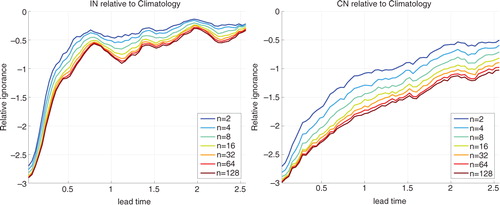
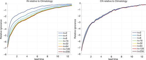
Predictability in a chaotic system is a property of a forecast system, not merely the underlying deterministic dynamical system. In addition to verifying observations from the target dynamical system (the ‘data generating mechanism’ whatever it may actually be), a forecast system includes the observational network (fixed and adaptive), full data assimilation scheme, dynamical simulation model(s), properties of the ensemble and the ensemble interpretation scheme, and so on; in short, every aspect of the operational forecast system that has any impact on the forecast generated. This means that one cannot quantify the predictability of the Moore–Spiegel system itself. The predictability, as reflected in the decay of forecast skill with lead time, of the Moore–Spiegel system under each of two different forecast systems is shown in Fig. 2. The two forecast systems are based on different data assimilation algorithms (namely IN and CN as noted above); these are introduced in the next two sub-sections. Note that the decay of predictability in the right panel is much slower than the decay in the left panel. Similarly, the utility of increasing the ensemble size can be expected to vary with other aspects of the forecast system, as demonstrated in the next sub-section. Such observations suggest that more systematic consideration of ensemble size in the design of forecast systems would be of value.

Fig. 2 Moore–Spiegel system. The decay of predictability with time of two forecasts systems of the Moore–Spiegel system. Ignorance relative to climatology is shown as a function of lead time for ensembles of size 2, 4, 8, 16, 32, 64 and 128. Lead-time is reflected by colour. The forecast systems differ in the data assimilation scheme used; Left: The inverse noise (IN) method. Right: The collapsed noise (CN) method. Note the forecast system using CN gives systematically more skilful forecasts. Note that the larger ensembles routinely show greater skill at each lead time for each system.

4.1.2. Inverse observational noise ensemble formation.

Multiple ensemble forecasts were made for the Moore–Spiegel system, launched from (near) 1024 observations separated in steps of 2.56 time units along a trajectory. These points in time, which reflect the system state, are the focus about which forecasts are initialised and are hereafter simply called ‘launch points’. Initial condition ensembles were formed about the observation at each launch time. Inverse observational noise ensembles were generated by perturbing each launch point with Gaussian innovations of the same covariance matrix as the observational noise [In this special case, the inverse noise (IN) model has the same covariance matrix as the observational noise)]. Each ensemble of simulations is iterated forward under the Moore–Spiegel system for a duration of 2.56 time units and interpreted as a density forecast; the kernel width and blending parameters were selected to minimise mean ignorance over a training-set of 1024 IN forecast–outcome pairs for each lead time and ensemble size.

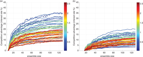
Figure 3 shows the competitive advantage increases as ensemble size increases. The left panel shows the competitive advantage relative to an ensemble of size 8, the right panel relative to an ensemble of size 16. Clearly increasing the ensemble size well above the value of 8 or 16 is beneficial; arguably it is still increasing at the largest ensemble sizes considered in these graphs (128). While noting that small ensembles were sufficient to provide a good root-mean-square estimate of the ensemble mean, Leith (1974) also suggested moving beyond root-mean-square error, and that a better measure would reflect maximising the user's expected gain. Inasmuch as the ignorance score reflects utility, our results are consistent with Leith's insight.

Fig. 3 Moore–Spiegel system with inverse noise. Graphs of competitive advantage when increasing the ensemble size relative to a reference ensemble size. Left: Reference ensemble-size is 8. Right: Reference ensemble-size is 16. The colour bars indicate lead time. Note that when the competitive advantage is sloping upward towards the right-hand side of each graph, the benefit of increasing the ensemble size is still increasing at the largest ensembles tested. At shorter lead times (dark blue) the benefit tends to be greater than longer lead times (dark red).

The panels in Fig. 4 reflect vertical slices through Fig. 3, one panel with ensemble size 32, the other with ensemble size 128. The right panels of Fig. 4 show the corresponding ignorance scores, illustrating the (inverse) relationship between ignorance and competitive advantage.

Fig. 4 Moore–Spiegel system with inverse noise. The two graphs on the left show the competitive advantage as a function of lead-time for an ensemble size of 32 relative to 16 as a functions of lead-time (top) and 128 relative to 16 (bottom). Each curve corresponds to a slice through Fig. 3. The IGN scores for the same comparisons are shown on the right. Note the symmetry between ignorance and competitive advantage [flipping over (y → −y) in a graph in the right column leads yields the pattern of a curve on the left].

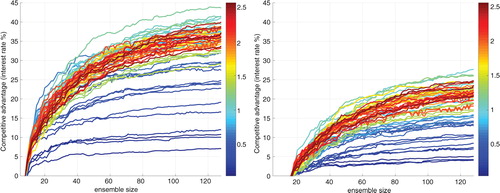
The competitive advantage gained by doubling the ensemble size as a function of the final ensemble size under IN is shown in the left panel of Fig. 5. Note that as the ensemble size is doubled, competitive advantage is positive at all lead times considered. Most of the higher lead times yield competitive advantages greater than 1 %.

Fig. 5 Doubling the ensemble size in the Moore–Spiegel system. Left: Graphs of competitive advantage gained by doubling the ensemble size of IN forecast systems as a function of the final ensemble size. Right: Graphs of competitive advantage gained by doubling the ensemble size of CN forecast systems as a function of the final ensemble size. Each line on a given graph corresponds to the forecast lead time according to the corresponding colour bar. Note that doubling the ensemble size is demonstrably beneficial at all lead times, and the (more expensive) CN-based forecast systems tend to benefit more than the IN-based systems, especially at longer lead times.

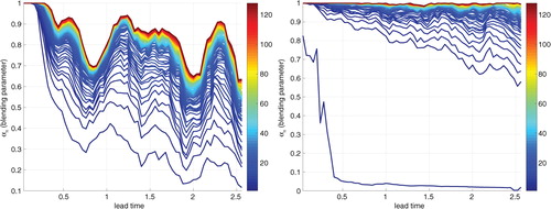
The left panel of Fig. 6 shows the blending parameter as a function of ensemble size for a forecast system using IN data assimilation. In general, the blending parameter tends to rise as a function of ensemble size. That is, the climatology is weighted more highly in smaller ensembles. Note however that at some intermediate lead times (those plotted as lighter blue and yellow, for instance) the value of α _n for large ensemble sizes falls below that of both shorter and longer lead time forecasts. This is shown more clearly in Fig. 7, where the blending parameter for various ensemble sizes is shown as a function of lead time. On the left, notice the oscillatory behaviour of the blending parameter (as a function of lead time), especially for larger ensemble sizes. This might be a feature of the chaotic nature of the underlying dynamics due to variations in predictability across time scales (Smith, 1994) or may be due to the macroscopic structure of this particular attractor. The decrease in the blending factor as a function of lead time reflects a number of different effects, from issues of data assimilation to model inadequacy. In light of this, a more effective ensemble formation scheme is considered in the next section.

Fig. 6 Moore–Spiegel system. Graphs of blending parameter (α _n ) versus ensemble size determined by minimising the average ignorance score over a forecast–outcome archive. Left: IN-based forecast systems. Right: CN-based forecast systems. Note the systematic increase of α _n with ensemble size in each panel. The colour bars on the right of each panel correspond to lead time.

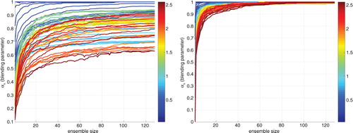
Fig. 7 Moore–Spiegel system. Graphs of blending parameter (α _n ) versus lead time under each of the two data assimilation strategies. Left: IN-based forecast systems. Right: CN-based forecast systems. In the IN-based systems the general decrease in α _n with lead-time is rather complex; nevertheless the value of α _n for these systems is systematically lower than that for the CN-based systems, and thus the weight on climatology is significantly greater. In the CN-based forecast systems, the decrease is more regular; interestingly at a given lead-time the value of α _n is greater for the larger lead-times. This suggests a potentially resolvable shortcoming in the CN data assimilation scheme. The colour bar on the right-hand side of each graph indicates the number of ensemble members.

4.1.3. Collapsed noise ensemble formation.

The dynamic of a dissipative chaotic system induces a natural measure (which sometimes falls on a strange attractor) in the system state space (Eckmann and Ruelle, 1985). This distribution would yield an ideal climatology in meteorological terms. For instance, the distribution of temperature at a given geographical point is the marginal distribution of a higher dimensional climatological distribution. Given a noisy observation of the state of the system, there will be a distribution consistent with both the observational uncertainty (the noise model) and the dynamics of the system (as reflected in the local detailed structure of the climatological distribution). Ideally, an accountable ensemble would be drawn from a set of indistinguishable states of a perfect model, states consistent with the observations, the dynamics and the noise model (Judd and Smith, 2004); only the simpler target of a dynamically consistent distribution (defined below) is attempted in this article.

In meteorology, obtaining the initial state (or distribution) is referred to as data-assimilation (e.g. see Lorenc, 1986; Kretschmer et al., 2015; Stull, 2015). Traditional data assimilation typically aims to determine a single state by minimising the misfit between a model trajectory and observations within the corresponding assimilation window. The benefit of increasing ensemble size can be expected to vary with the data assimilation scheme used to construct the ensembles. Sampling the set of indistinguishable states is computationally costly. Hansen and Smith (2001) suggested that one might sample an alternative distribution in which the states are ‘more consistent’ with the model dynamics than in the IN approach yet less expensive than sampling the natural measure. Given initial candidates drawn from an IN distribution at the beginning of an assimilation window, it was suggested that one retain candidates weighted by their consistency with all the observations in an assimilation window yielding a dynamically consistent initial distribution. The method used in subsequent discussions employs a weaker constraint: the same initial candidates are selected at the beginning of the assimilation window; whether or not they are included in the ensemble is then based only on their distance to observation at the launch time (the most recent end of the assimilation window). Details of this ‘final-time CN’ algorithm are in Appendix A.

The competitive advantage graphs for IN-based forecast systems and CN-based forecast systems are shown in the right panel of Fig. 5. Notice that the longer lead-time performance under CN benefits more from increases in the ensemble size than under IN. In particular, when the ensemble size doubles to 128, the longer lead time graphs yield competitive advantage of at least 2 % per trial. It is evident that doubling the ensemble size generally benefits the forecast system using CN more than the one using IN at longer lead times and larger ensemble sizes. At the shortest lead times (<0.05) the forecast system using IN shows a larger benefit.

The quality of the ensemble formation scheme is also reflected in the blending parameter (see Fig. 6), which increases as the ensemble size increases: the forecasts have increased skill and the ensemble component of the forecast distribution is weighted more heavily relative to climatology. This increase with ensemble size tends to be slower for longer lead-time forecasts; note also the behaviour of the blending parameter. Graphs of the blending parameter corresponding to the CN ensemble shown in the right panels of Figs. 6 and 7 lie in striking contrast to those corresponding to IN ensembles inasmuch as the CN blending parameters increase, approaching one for all lead times (signalling a significant increase in information content of the distribution of ensembles members), while the blending parameters of the IN ensembles appear to saturate at α _n significantly less than one.

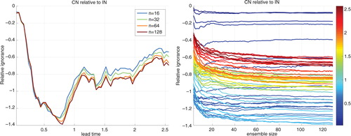
Values of the blending parameter α _n which are less than one suggest imperfection somewhere in the forecasting system; possible imperfections include flawed ensemble initialisation strategies, suboptimal parameter selection, structural model error (Orrel et al., 2001), a poor ensemble interpretation and an ensemble of finite size. Chaos cannot be blamed for these imperfections since a perfect initial ensemble evolved forward in time under a perfect model with the correct parameters can yield forecast distributions that are perfectly consistent with observations of the system (i.e. they are accountable; their performance is hindered only by containing a finite number of members). Figure 6 suggests that in this case significant improvement in forecast skill is achieved by improving the data assimilation scheme and increasing the ensemble size. The improvement in skill using CN data assimilation is clear in each panel of Fig. 8. The left panel shows the skill of CN relative to IN as a function of lead-time for several different ensemble sizes. In every case, the value is negative indicating that CN outperforms IN, and for longer lead times this relative advantage increases as the ensemble size increases, although the increase is smaller for larger ensemble sizes. The right panel shows the skill of CN-based systems relative to IN-based systems as a function of ensemble size, for a variety of lead-times. Note that at longer lead-times (coloured red or orange) the curves appear to be downward sloping even at the largest ensemble sizes; this would indicate that the more expensive data assimilation scheme (CN) benefits more (obtains a larger α _n ) from increasing the ensemble size even at the largest sizes tested.

Fig. 8 Contrasting skill due to data assimilation scheme: Moore–Spiegel system. The skill of competing forecast systems which differ only in the data assimilation scheme is contrasted in the Moore–Spiegel system: each panel shows IGN of CN-based forecasts relative to those of IN-based forecasts, thus negative values imply more skill in the CN method. Note that all values are negative. Left: Ignorance as a function of lead time for four ensemble sizes (16, 32, 64 and 128). Note that the forecast system using CN gains additional skill above the one using IN as the ensemble size increases. Right: Ignorance as a function of ensemble size for a variety of lead times (as indicated by the colour bar on the right-hand side of the panel). Note that the benefit of using CN is greatest in the medium range, lead times between 0.5 and 0.9; while the advantage continues to exceed half a bit (a 40 % gain in probability, on average) at longer lead times, it is less than a tenth of a bit at short lead times. This suggests that the CN data assimilation might require improvement (to justify its added cost) if the focus is on shorter lead times. Also note in the right panel that for longer lead times (reddish) the skill curves are still sloping down even at the largest ensembles tested, indicating that the CN-based forecasts are improving faster as the ensemble size is increased even at the largest ensembles tested.

The increase in competitive advantage (under CN) in Fig. 5 indicates that doubling the ensemble size can yield a competitive advantage of 2.5 % even at the largest ensemble sizes considered. Comparing these with the IN case in Fig. 5, it is clear that at longer lead times, more improvement is made under CN. Graphs of the competitive advantage obtained when competing with a forecast system issuing odds based on ensemble sizes of 8 and 16 respectively are shown in Fig. 9.

Fig. 9 Moore–Spiegel system with collapsed noise. Graphs of competitive advantage when increasing the ensemble size relative to a reference ensemble-size. Left: Reference ensemble-size is 8. Right: Reference ensemble-size is 16. Contrasting this figure with its counterpart (Fig. 3) suggests that for all but the shortest lead times, using the CN algorithm increases the gain obtained by these increases in ensemble size. The colour bar on the right-hand side of each graph indicates the lead time.

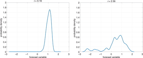
Forecast distributions derived from the same initial ensemble of 128 members are shown in Fig. 10; two lead times are shown. Notice that the longer lead time distribution does not appear to be Gaussian; in any event a Gaussian distribution evolving under a non-linear model will inevitably become non-Gaussian. The results of the previous section suggest that (relevant) complexity in the longer lead time distributions will increase the value-added by increasing the ensemble size. In numerical weather prediction, it is common to interpret an ensemble as a Gaussian distribution; this procedure can lead to relatively poor forecast skill (Brocker and Smith, 2008). The results presented here reinforce the suggestion that kernel dressing is to be preferred: ensemble interpretations which merely fit predictive distributions using symmetric unimodal distributions can reduce the utility (information content) available in larger ensemble sizes.

Fig. 10 Moore–Spiegel with collapsed noise. Two illustrative forecast distributions corresponding to the same initial ensemble; the ensemble size n=128. The left panel at lead time τ=0.16 shows a distribution that might be well described as normally distributed. The right panel, at longer lead time τ=2.56, would be less well described by a normal distribution.

5. Imperfect model scenario: a physical circuit

Insights based upon mathematically known dynamical systems do not always generalise to real-world systems; this is no doubt in part due to their having a well-defined mathematical target in the first case. It is of value to evaluate claims in forecasts of actual systems. An electronic circuit designed to mimic the Moore–Spiegel system is used for this purpose. Voltages corresponding to the three variables were collected with a sampling frequency of 10 kHz (i.e. every 0.1 ms). A data-based model of the circuit was constructed using radial basis functions in a four-dimensional delay space, based on the voltage signal that mimics the z variable in the Moore–Spiegel system. Further details of the circuit and this model can be found in Machete (2013b). As before, 1024 launch points were considered, allowing 64 time steps between consecutive launch points. A maximum forecast lead time of 128 time steps is considered, with ensemble of size n where n takes on integer values within the set {1,2,…,256}. In terms of the ignorance of forecasts relative to climatology, the predictability of the circuit at the longest lead time considered (128 time steps) is comparable to that of 8-day ahead weather forecasts (Brocker and Smith, 2008) under this model.

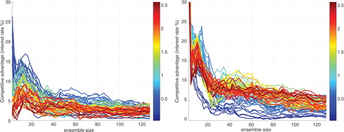
First consider IN ensembles where, following earlier work (Machete and Moroz, 2012), a standard deviation of 10⁻² was used. Graphs demonstrating the value of doubling the ensemble size in this case are shown in Fig. 11. As before, the different lines correspond to lead times according to the colour bar on the right-hand side. Note that there is less improvement from increasing the ensemble size at longer lead times. This observation is more evident on graphs of competitive advantage over ensemble sizes of 8 and 16 shown in Fig. 12. The lead times considered all correspond to forecasts with predictive skill relative to climatology.

Fig. 11 Circuit with inverse noise. Left: Graphs of competitive advantage of an ensemble versus an ensemble half its size. All forecast results in this article are out of sample. Right: Graphs of blending parameter versus ensemble size, note that α _n saturated (the curve goes flat) at smaller ensemble sizes than in the case of IN-based forecasts of Moore–Spiegel. Each line on a given graph corresponds to the forecast lead time according to the corresponding colour bar.

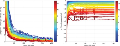
Fig. 12 Circuit with inverse noise. Graphs of competitive advantage when increasing the ensemble size relative to a reference ensemble-size. Left: Reference ensemble-size is 8. Right: Reference ensemble-size is 16. The colour bars indicate lead time. Note that when the competitive advantage is sloping upward towards the right-hand side of each graph, the benefit of increasing the ensemble size is still increasing at the largest ensembles tested. At shorter lead times (dark blue) the benefit tends to be more than longer lead times (dark red). The colour bar on the right-hand side of each graph indicates the lead time. The occasional glitches (short, sharp drop-outs of low skill) are due to a well understood flaw in our automated kernel-selection algorithm.

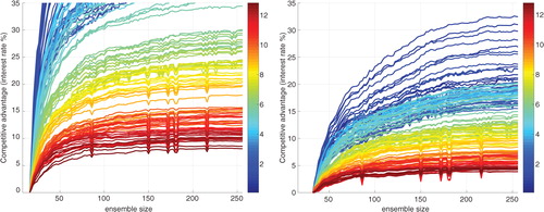
At the longer lead times, the ensembles under the model dynamics represent the dynamics of the target system less well. This decreases the benefit from increasing the ensemble size. Nevertheless, the benefit of ensembles with more than 16 members remains significant in this imperfect model case. Note the upward sloping lines on the right panel of Fig. 12, which indicate that forecasts are improved by increasing the ensemble size even at the largest ensembles considered. For shorter lead-times this improvement is striking.

6. Quantifying reliability, resolution and other properties of forecast distributions

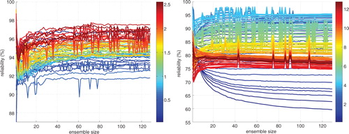
Probability distributions have many properties. Some of these properties (like IGN) reflect their information content regarding target outcomes, while other properties (like variance) reflect only properties of the distribution itself. Only forecast skill reflects the value of the forecast. In this section, other properties are considered. A probability forecast system is arguably reliable if its forecast probabilities are consistent with the relative frequency(s) of the outcome observed. Of the many measures of reliability, a measure based on the probability integral transform, reliability _PIT , is considered below. Resolution is quantified by the area under the ROC curve, denoted resolution _ROC . These measures are defined in Appendix B.1. Note that the application of such summary statistics often requires abandoning the evaluation of full probability forecasting of continuous variables, as those statistics consider merely binary (or other few-tile) forecasts. Graphs of reliability _PIT for the blended distributions are shown in Fig. 1 and for Moore–Spiegel System in Fig. 13.

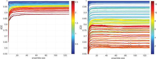
Fig. 13 Quantifying reliability _PIT . Graphs of reliability _PIT as a function of ensemble size. Left: Moore–Spiegel system under CN-based forecast systems. Right: Circuit under IN-based Forecast systems. Here forecasts of the circuit, for which the model is imperfect, display two qualitative differences from the Moore–Spiegel system and the mixture distributions shown in Fig. 1. First, at the shortest lead times (dark blue) reliability _PIT decreases significantly with ensemble size. Second, at the longest lead times (orange and red) there is a slow decrease in reliability _PIT rather than a plateau. The occasional glitches are due to a well understood flaw in our automated kernel selection algorithm.

The lower right panel of Fig. 1 shows reliability _PIT for the two Gaussian mixture distributions of Section 3 as functions of ensemble size. In both cases, as the ensemble size increases from one, reliability _PIT first decreases (until an ensemble size of about eight) and then increases monotonically. The reliability _PIT of the Gaussian distribution falls more steeply and rises more slowly than that of the mixture.

Contrast this graph with graphs of reliability _PIT of forecasts of the Moore–Spiegel system and the circuit in Fig. 13. As in the density estimation case, these graphs generally show an initial decrease in reliability _PIT with increasing ensemble size, and followed by a steady increase. This general behaviour is seen at all lead times considered in the Moore–Spiegel case. Interestingly, the early lead time forecasts of the circuit (darker blues in the right panel of Fig. 13) show a different behaviour in that the reliability _PIT continues to decrease with increasing ensemble size. Observations like this are the value of the reliability and resolution measures, as they can inspire insights that lead to the improvement of forecast skill.³ Also note the decrease in reliability _PIT at longer lead times for the circuit (right panel of Fig. 13). This decrease is effectively monotonic, in contrast to the pure density estimation. While the impact of model error is expected to increase with lead time, it is unclear why as ensemble size increases a good ensemble interpretation scheme would not counter this decrease in reliability _PIT , resulting in values of reliability _PIT which were roughly constant.

The competitive advantage gained by increasing ensemble size occurs not, of course, because the forecast distributions achieve a better reliability _PIT or become sharper per se, but rather because more probability is placed on the outcome as the ensemble size is increased. Under CN, the sharpness of forecast distributions (not shown) increases a good deal at shorter lead times, highlighting the potential benefits of an effective data assimilation scheme. It is critical to note, however, that an increase in sharpness only adds to information content or the economic benefit if the relative ignorance decreases.

Richardson (2001) and Weigel et al. (2007) considered the effects of ensemble size on reliability (or calibration) based on the decomposition of the Brier score, effectively assessing probabilistic calibration. One should not, however, expect perfectly calibrated forecasts in practice (Gneiting et al., 2007; Machete, 2013a). Even under a perfect model, perfect calibration would require that the initial distributions be accountable, that is consistent both with the long-term dynamics of the target system and with the observations given the statistics of the observational noise (Smith, 1995). This is unlikely to be the case (Judd and Smith, 2004).

Note that many properties of the distributions (such as ROC curves shown in Fig. 14) saturate at relatively small ensemble sizes, while the skill of the forecast continues to increase, illustrating that those measures do not reflect skill. It is the skill of a forecast system, neither its components nor the averaged properties of the forecast distributions, which determines forecast value.

Forecast skill is best reflected by (a subset of) proper skill scores. The limited utility of reliability per se is not surprising; note for example that a climatological distribution is reliable by construction, yet it will be outperformed by a less reliable probability distribution conditioned on current observations with significantly more skill. This insight is not new and Bross highlighted this point over half a century ago [note that Bross (1953) used the word ‘validity’ rather than ‘reliability’]. Reliability, however defined, is but just one aspect of a forecast system. A more complete investigation of various measures of reliability (and other forms of calibration) and of resolution would be of value.

7. Discussion and conclusions

How might this study, considering only low-dimensional mathematical systems and data from a physical circuit, aid the design of operational forecast systems? First, it argues strongly for the evaluation of information provided by larger ensembles at the design stage (Palmer et al., 2004; Doblas-Reyes et al., 2005; Smith et al., 2014). There has been resistance to considering more than nine members in these hindcast studies; the restrictions this placed on evaluating the value of ENSEMBLES⁴ are documented in Smith et al. (2014). While a detailed investigation of ensemble design is beyond the scope of this article, it is noted in passing that a more effective experimental design need not require the computational cost of running massive ensembles for every hindcast launch date. Second, improvements in the ensemble formation scheme (data assimilation designed explicitly to generate ensembles) can significantly increase the information provided by larger ensembles. More generally, it is conjectured that the better the simulation model, the greater the benefit of increasing the size of the ensemble. Computational resources may be fixed, of course, but a more informative forecast system arguably justifies increased computational resource.

The longstanding question of the appropriate size for a forecast ensemble-size has been considered both in PMS and in the imperfect model scenario. Model inadequacy and the particular ensemble-formation scheme place a limit on the gain achievable by increasing the ensemble size. A good ensemble formation scheme and a good ensemble interpretation can each enhance the benefit of increasing the ensemble size well above 16 members. Some previous studies have focused on the effect of one additional member on the quality of the ensemble (Richardson, 2001; Ferro et al., 2008) in a root-mean-square sense. Even in this context, Smith et al. (2014) have shown that probabilistic evaluation can lead to insights different from those where the evaluation is restricted to the ensemble mean as a point-forecast.

The approach in this article is more information theoretic: It assessed the effect of doubling the ensemble size on probabilistic-forecast quality as measured by ignorance (Good's logarithmic score), which reflects the information contained in the forecast. In PMS under a good ensemble formation scheme, doubling the ensemble size still resulted in a non-trivial improvement in competitive advantage, averaging an increase of at least 2 % (per forecast), even for ensembles of size 128. If this first appears to be only a small advantage, consider the fact that, compounded daily, an initial investment would be multiplied by a factor of 1377 after one year! The competitive advantage was greater on longer lead times. An analysis of traditional kernel density estimation suggests that inasmuch as the magnitude of the advantage varies with properties of the underlying distribution, more complex distributions benefit more from increasing the ensemble size than simple unimodal distributions. This is consistent with much of the competitive advantage at longer lead times arising from the non-Gaussian nature of the forecast distributions at these lead times. Cases where complicated forecast distributions systematically outperform Gaussian forecast distributions out of sample reflect this effect, even when traditional null hypothesis tests (given small ensembles) fail to detect a statistically significant departure from normality. In any case, given a non-linear model, an initially Gaussian distribution will evolve to become non-Gaussian (McSharry and Smith, 1999).

Outside PMS, forecasts at longer lead times benefit less from increasing the ensemble size. This is consistent with structural model error having a greater impact at longer lead times than at shorter lead times: at longer lead times even arbitrarily large ensembles would provide limited information regarding the relevant target distribution.

The effect of improved data assimilation within PMS can be gleaned from the right panel of Fig. 8. Notice that for each ensemble size shown the relative ignorance is negative, signalling that there is improvement in the probabilistic forecast skill due to implementing the data assimilation scheme. Also note that this relative advantage is maintained as the ensemble size increases (each curve is fairly horizontal for all but the smallest ensemble sizes).

While only one target variable has been considered in determining how large an ensemble size should be, the approach above can be extended to the multivariate forecast target case. Forecast distributions for different target variables may have very different properties (some may be positive definite, for instance) suggesting that the desired ensemble size for different target variables may differ as well, unless an elegant ensemble interpretation is available. The use of a novel ensemble-formation scheme based upon the work of Hansen and Smith (2001) illustrates significant improvements given a more effective ensemble formation scheme. The fact that the simple data assimilation scheme employed above will no doubt prove inferior to alternative ensemble-formation schemes does not detract from our point: better ensemble formation schemes are expected to increase the benefit of increasing ensemble size.

Fig. 14 Resolution _ROC . Left: Graphs of the area under the ROC curve , resolution _ROC , which is considered a measure of resolution. Left: For the Moore–Spiegel system under CN-based forecast systems. Right: For the Circuit under IN-based forecast systems. The colour bar on the right-hand side indicates the forecast lead time.

A central argument of this article is well-captured in Fig. 15, which shows the skill of two forecast systems of the circuit with lead time; each system is shown for a variety of ensemble sizes. In each panel there is an effectively monotonic increase in skill each time the ensemble size is doubled. The uniformity of this improvement is much clearer in the left panel, which reflects the skill of the forecast systems using IN assimilation. Note that the improvement shown in the right panel, which reflects the skill of the forecast systems using CN assimilation, is rather different: the gain from doubling the ensemble size is much less in absolute terms (bits). In addition, the gain in skill in moving from IN data assimilation to CN data assimilation dwarfs the improvement obtained after significant increases in the ensemble size of the forecast system using IN. The argument of this article is not that larger ensembles are always justified, but rather that decisions regarding resource allocation and forecast system design are better informed when the information gain of altering the ensemble size (and data assimilation method) are explored explicitly. The cost of quantifying the value of larger ensembles is, relatively, modest. In the case of Fig. 15, increasing the ensemble size to (at least) 256 increases the skill of the forecast, and at the same time, the larger investment required to change data assimilation scheme yields a much larger improvement in the information content of out-of-sample forecasts.

Fig. 15 Decay of predictability of the circuit in two forecast systems based on different data assimilation schemes. IGN score of forecasts of the circuit relative to climatology for eight ensemble sizes. The two forecast systems use different data assimilation methods. Left: A inverse noise (IN)-based forecast system. Right: Collapsed noise (CN)-based forecast system, with an assimilation window of two steps. Note that the gain from merely moving from an IN-based forecast system to a CN-based forecast system alone is much greater than the gain from increasing the ensemble size by a factor of 128 in the IN-based forecast system.

In forecasts of mathematical chaotic systems and in forecasts of a physical system, more information can be gleaned from ensemble forecasts by increasing the ensemble size well beyond ‘16’. While the general thrust of these arguments hold in forecasting more complicated physical systems, the quantitative results will depend on model quality, the data assimilation scheme, the ensemble interpretation method and the target system observable. We hope this article has given sufficient evidence to justify further exploration of the information larger ensembles provide in operational forecast systems.

8. Acknowledgements

We thank Hailiang Du, Emma Suckling and Edward Wheatcroft for reading earlier versions of this article and giving useful feedback. Lyn Grove improved the readability of the article significantly. This research was supported by the LSE Grantham Research Institute on Climate Change and the Environment and the ESRC Centre for Climate Change Economics and Policy, funded by the Economic and Social Research Council and Munich Re. Support of Climathnet is also acknowledged. Feedback from three anonymous reviewers helped improve the manuscript, and we are particularly grateful to one of these reviewers for insightful comments that improved both presentation and content. LAS gratefully acknowledges the support of the Master and Fellows of Pembroke College, Oxford.

Notes

1 For a probability q, the ‘to odds’ are defined as , whereas Kelly's ‘for odds’ are defined as .

2 The system is integrated with a fourth-order Runge–Kutta method, initialised with a randomly chosen initial condition near the origin; transient states were discarded. The integration time step used is 0.01 and states were recorded every four steps; thus, the time step between any successive data points is 0.04. The observations are true states corrupted with zero-mean, uncorrelated additive Gaussian noise such that each variable had a signal to noise ratio of 10:1. (The standard deviation of the observational noise added to the true z variable is 0.1; in the Moore–Spiegel system σ _z ≈1.13.)

3 It can be argued that, in the case of and only of binary forecasts, reliability measures can be used to ‘recalibrate’ the forecast once the forecast–outcome archive is sufficiently large. In cases where the causes of miscalibration are robust (unchanging), this can be approached simply by forecasting the relative frequency corresponding to the actual forecast system. As the focus of this article is on evaluating probability forecasts of continuous variables, this avenue is not pursued further. We are grateful to an anonymous reviewer for stressing the possibility of doing so.

4 ENSEMBLES was a large multi-model seasonal hindcast project (Alessandri et al., 2011, and citations thereof).

5 Given two vectors, a=(a₁,…,a_m) and b=(b₁,…,b_m), the inner product of the two vectors is . It follows that 〈a,e_i〉=a_i.

9. Appendix

A. Data assimilation

Given a time series of observations { s (t)} _t≥0 and that the underlying dynamics are described by the function ϕ ( x ,t) where x ∈ ℜ ^m (the state vector is m-dimensional) and the initial state is x (0)= x ₀, then the state at time t is given byA.1

where x _t and x (t) have the same meaning. Usually, one cannot know the true state x (t). If h is the observation function, thenA.2

where ɛ _t is the observational error. In the algorithm given below, the observation function is taken to be the identity operator and the uncertainty solely due to additive noise. Assume that and , that is, the observational errors have no bias and are spatially uncorrelated. Consider an initial observation and let e _i be a unit vector whose ith entry is one and the rest of the entries are zero. The parameter δ _i is the standard deviation of the observational noise corresponding to the ith coordinate. Typically, one has a non-linear model of the model dynamics φ (·,t) so that given a point z ₀, we can iterate it forward under the dynamics to obtain z _t = φ ( z ₀,t). In the perfect model scenario (PMS), φ (·,t) coincides with ϕ (·,t). Data assimilation then is a process of (often using the dynamical model) estimating initial conditions which define ensemble members. In the following algorithm of our simplified data assimilation scheme, j_max is a fixed integer denoting the maximum number of searches for a collapsed noise (CN) ensemble member, j is the integer that counts the number of searches for initial ensemble members and τ _a is the length (in time) of the assimilation window. Denote a Gaussian random vector by , where , and fix an integer k, which is the number of standard deviations within which an assimilation point is considered indistinguishable from the launch point . Let be an initial ensemble at the launch point. The number of ensemble members is denoted by . The algorithm is given below:

1. Set and j=0.

2. Perturb the observation s (t₀ – τ _a ) to obtain a new point y = s (t₀ – t _a )+ ξ and set j=j+1.

3. If j≤ j_max, compute φ ( y ,τ _a ) and go to (5).

4. If j>j_max, generate a new vector ξ to obtain a new point and set , j=0 and then go to (6).

5. If for all i, set ⁵ and go to (6).

6. If , then stop. Otherwise if j=j_max set j=j_max+1 and go to (4) else if j<j_max go to (2).

The aim of the above ensemble formation procedure is to evolve a random set of initial states near the observations at time t=t₀ – τ _a forward in time to t=t₀, and then use those which remain consistent with the observations at (up to) t=t₀ for the ensemble. This effectively collapses onto a set of states that are dynamically consistent with the system's dynamics. Step (1) sets the initial ensemble within the neighbourhood of a current observation to an empty set. Step (2) generates random states at the beginning of the assimilation window that are consistent with the observational error model (A2). Step (3) generates a potential member of the initial ensemble using the model dynamics. Step (4) curtails the search if an insufficient number of neighbours have not been found in good time; the integer j_max defines the threshold that restricts the maximum time allocated for the search. Step (5) assesses whether the point at the end of the assimilation window is within some neighbourhood of the current observation; if it is, then it is taken to be a member of the CN initial ensemble, B( s ₀). The resulting initial ensemble B( s ₀) should be approximately distributed more consistently with the climatological distribution and be consistent with the model dynamics. Another possibility to avoid the cost of long searches is to adjust k for this initial condition; this option will be reported in future work. Alternatively, the search for members stops when the required ensemble size is reached [Step (6)].

In the experiments reported above, j_max=512 with k=3 for MS system and k=1 for the circuit, τ _a =6.4 for the MS system (and two time steps for the circuit); n took on each integer value in the set {1,2,…,128} for the MS system and n ∈ {1,2,…,256} for the circuit. A time series of the Moore–Spiegel system was generated such that the time step between successive points was 0.04. From this time series, 1024 launch points were sampled such that there were 128 time steps between successive launch points. Ensemble forecasts were then made from the 1024 launch points up to lead times of 128 time steps, based on initial ensembles being generated via the CN scheme.

B. Properties of forecast distributions

B.1. Reliability

Statistical consistency between the forecast probabilities and corresponding outcomes is a desirable property of probability forecasts; one aspect of this property is termed reliability (Brier, 1950) in meteorology and calibration in economics (Dawid, 1984; Diebold et al., 1998; Gneiting et al., 2007). The meteorological community uses ‘reliability diagrams’ to assess reliability (Brier, 1950; Brocker and Smith, 2007) whilst the economics community tends to use probability integral transforms. A reliability diagram is obtained by plotting predicted probabilities against observed relative frequencies: if the forecast system is reliable, the relative frequencies will lie near the diagonal, the relevant distance depending on the number of forecasts, the precise probabilities and so on. Brocker and Smith (2007) provided a straightforward approach to interpreting reliability diagrams and noted that visual inspection is at best uninformative. The probability integral transform provides one summary statistic which can be used to compare the reliability of two forecasting systems (Dawid, 1984).

Consider a sequence of density forecasts, , and corresponding observations (i.e. outcomes) . If the cumulative distribution function for each f _t (x) is F _t (x), then the corresponding probability integral transform is given by z _t =F _t (x _t ). In finance and economics, a forecasting model is said to be correctly specified (or perfectly calibrated) if (Diebold et al., 1998; Corradi and Swanson, 2006), where ‘U[0,1]’ stands for uniformly distributed on the interval 0 to1. Machete (2013a) argued that this requirement is not satisfied by operational forecasting models.

The aim is a summary measure of reliability for imperfect forecast systems. First note that a sequence of probability integral transforms can be used to form an empirical distribution functionB.1

Reliability can then be assessed by computing the L ¹ norm (Hora, 2004),B.2

This norm is a measure of miscalibration and details of its computation can be found in Hora (2004). Noting that the norm attains the minimum of 1/4T and the maximum of 1/2, Hora (2004) inverts and rescales the norm to obtain a measure of probabilistic calibration, which is a measure of the degree of reliability. This measure is given byB.3

which takes values between 0 and 100 %, larger values corresponding to greater reliability; this measure or statistic is referred to as reliability _PIT due to its dependence on probability integral transforms and it is positively oriented. Alternative measures of reliability can be defined.

Note that Machete (2013a) suggested an alternative form of calibration proposed by Gneiting et al. (2007), called marginal calibration. Given a sequence of forecasts , a forecasting system is said to be marginally calibrated ifB.4

While beyond the scope of this article, further investigation of marginal calibration is of interest.

B.2. Resolution

In the recent work of Brocker (2015), a forecasting scheme is said to have no resolution if the forecasts are independent from the observations. This definition is said to be consistent with that of the WWRP/WGNE Joint Working Group on Forecast Verification. Equivalently, a forecasting scheme has no resolution if the conditional probability of the forecast given the observation does not depend on that observation (Brocker, 2015).

The resolution of a binary forecasting scheme can be quantified by computing the area under an ROC curve. This area is applicable to binary observations or events (Brocker, 2015), but extensions are given in Mason and Graham (2002). In order to present this metric, let Y be an observation with Y ∈ {0,1}. Assume that Λ is the forecast probability that Y=1. Hence the probability that Y=0 is 1 − Λ. Here Λ is taken to be a random variable taking values between 0 and 1.

The hit rate can then be defined asB.5

and the so-called false-alarm rate asB.6

Forecasts and observations are independent provided H(λ)=F(λ) for all λ ∈ [0,1] (Brocker, 2015). Hence a forecasting system has no resolution if this equality holds. Furthermore, the ROC curve is simply a graph of H against F. It is a monotonic increasing function whose shape depends on the statistics of Λ and Y. The foregoing equality can be tested using the Mann–Whitney U-statistic, which statistic is an estimate of the area under an ROC curve up to some factors. To estimate this statistic, given the data set , sorted such that the Λ's are in ascending order, the quantityB.7

is an estimate of the area under an ROC curve, with M₁ being the sum of all values of Y and M₀=M – M₁. Note that the bracketed term in eq. (B.7) is the Mann–Whitney statistic. In computations for quantifying the resolution of a forecasting scheme, Y=1 will be the event that the observation is less than the climatological mean. The statistic for resolution is called resolution _ROC and it is positively oriented.

References

- Alessandri A. , Borrelli A. , Navarra A. , Arribas A. , Deque M. , co-authors . Evaluation of probabilistic quality and value of the ENSEMBLES multimodel seasonal forecasts: comparison with DEMETER. Mon. Weather Rev. 2011; 139: 581–607.
- Balmforth N. J. , Craster R. V . Synchronizing Moore and Spiegel. Chaos. 1997; 7(4): 738–752.
- Bates J. M. , Granger C. W. J . The combination of forecasts. Oper. Res. Soc. 1969; 20(4): 451–468.
- Brier G. W . Verification of forecasts expressed in terms of probability. Mon. Weather Rev. 1950; 78(1): 1–3.
- Brocker J . Resolution and discrimination – two sides of the same coin. Q. J. Roy. Meteorol. Soc. 2015; 141: 1277–1282.
- Brocker J. , Smith L. A . Increasing the reliability of reliability diagrams. Weather Forecast. 2007; 22(3): 651–661.
- Brocker J. , Smith L. A . From ensemble forecasts to predictive distribution functions. Tellus A. 2008; 60(4): 663–678.
- Bross I. D. J . Design for Decision: An Introduction to Statistical Decision-Making. 1953; New York: Macmillan.
- Buizza R. , Palmer T. N . Impact of ensemble size on ensemble prediction. Mon. Weather Rev. 1998; 126: 2503–2518.
- Chatfield C . Time Series Forecasting. 2001; London: Chapman and Hall.
- Corradi V. , Swanson N. R . Elliott G. , Granger C. W. J. , Timmermann A . Predictive density evaluation. Handbook for Economic Forecasting. 2006; North-Holland: Elsevier. 197–284.
- Dawid A. P . Present position and potential developments: some personal views: statistical theory: the prequencial approach. J. Roy. Stat. Soc. A. 1984; 147(2): 278–292.
- Diebold F. X. , Gunther T. A. , Tay A. S . Evaluating density forecasts with application to financial risk management. Int. Econ. Rev. 1998; 39(4): 863–883.
- Doblas-Reyes F. J. , Hagedorn R. , Palmer T. N . The rationale behind the success of multi-model ensembles in seasonal forecasting. Part II: calibration and combination. Tellus A. 2005; 57: 234–252.
- Eckmann J. P. , Ruelle D . Ergodic theory of chaos and strange attractors. Rev. Mod. Phys. 1985; 57: 617–653.
- Ferro C. A. T . Fair scores for ensemble forecasts. Q. J. Roy. Meteorol. Soc. 2014; 140(683): 1917–1923.
- Ferro C. A. T. , Jupp T. E. , Lambert F. H. , Huntingford C. , Cox P. M . Model complexity versus ensemble size: allocating resources for climate prediction. Philos. Trans. Roy. Soc. 2012; 370: 1087–1099.
- Ferro C. A. T. , Richardson D. S. , Weigel A. P . On the effect of ensemble size on the discrete and continuous ranked probability scores. Meteorol. Appl. 2008; 15: 19–24.
- Gneiting T. , Balabdaoui F. , Raftery A. E . Probabilistic forecasts, calibration and sharpness. J. Roy. Stat. Soc. B. 2007; 69(2): 243–268.
- Good I. J . Rational decisions. J. Roy. Stat. Soc. B. 1952; 14(1): 107–114.
- Hagedorn R. , Smith L. A . Communicating the value of probabilistic forecasts with weather roulette. Meteorol. Appl. 2009; 16(2): 143–155.
- Hansen J. A. , Smith L. A . Probabilistic noise reduction. Tellus A. 2001; 55(5): 585–598.
- Hora S. C . Probability judgements for continuous quantities: linear combinations and calibration. Manage. Sci. 2004; 50(5): 597–604.
- Judd K. , Smith L. A . Indistinguishable states I: perfect model scenario. Physica D. 2001; 151: 125–141.
- Judd K. , Smith L. A . Indistinguishable states II: the imperfect model scenario. Physica D. 2004; 196: 224–242.
- Kelly J. L . A new interpretation of information rate. Bell Syst. Tech. J. 1956; 35(4): 916–926.
- Kretschmer M. , Hunt B. R. , Ott E. , Bishop C. H. , Rainwater S. , co-authors . A composite state method for ensemble data assimilation with multiple limited-area models. Tellus A. 2015; 67: 26495.
- Lalley S. P . Beneath the noise, chaos. Ann. Stat. 1999; 27: 461–479.
- Leith C. E . Theoretical skill of Monte Carlo forecasts. Mon. Weather Rev. 1974; 102(6): 409–418.
- Leutbecher M. , Palmer T. N . Ensemble forecasting. J. Comput. Phys. 2008; 227: 3515–3539.
- Lorenc A. C . Analysis methods for numerical weather prediction. Q. J. Roy. Meteorol. Soc. 1986; 112: 1177–1194.
- Lorenz E. N . Deterministic non-periodic flow. J. Atmos. Sci. 1963; 20: 130–141.
- Lorenz E. N . Predictability of a flow which possesses many scales of motion. Tellus. 1969; 21: 289.
- MacEachern S. N. , Berliner L. M . Asymptotic inference for dynamical systems observed with error. J. Stat. Plan. Inference. 1995; 46: 277–292.
- Machete R. L . Modelling a Moore-Spiegel Electronic Circuit: The Imperfect Model Scenario. 2008; University of Oxford. DPhil Thesis.
- Machete R. L . Early warning with calibrated and sharper probabilistic forecasts. J. Forecast. 2013a; 32(5): 452–468.
- Machete R. L . Model imperfection and predicting predictability. Int. J. Bifurcat. Chaos. 2013b; 23(8): 1330027.
- Machete R. L. , Moroz I. M . Initial distribution spread: a density forecasting approach. Physica D. 2012; 241: 805–815.
- Mason S. J. , Graham N. E . Areas beneath the relative operating characteristics (ROC) and relative Operating levels (ROL) curves: statistical significance and interpretation. Q. J. Roy. Meteorol. Soc. 2002; 128: 2145–2166.
- McSharry P. E. , Smith L. A . Better nonlinear models from noisy data: attractors with maximum likelihood. Phys. Rev. Lett. 1999; 83(21): 4285–4288.
- Moore W. D. , Spiegel E. A . A thermally excited nonlinear oscillator. Astrophys. J. 1966; 143: 871–887.
- Muller W. A. , Appenzeller C. , Doblas-Reyes F. J. , Liniger L. A . A debiased ranked probability skill score to evaluate probabilistic ensemble forecasts with small sizes. J Clim. 2005; 18: 1513–1522.
- Orrel D. , Smith L. A. , Barkmeijer J. , Palmer T. N . Model error in weather forecasting. Nonlinear Process. Geophys. 2001; 8: 357–371.
- Palmer T. N. , Alessandri A. , Andersen U. , Cantelaube P. , Davey M. , co-authors . Development of a European multimodel ensemble system for seasonal-to-interannual prediction (DEMETER). Bull. Am. Meteorol. Soc. 2004; 85: 853–872.
- Palmer T. N . Predicting uncertainty in forecasts of weather and climate. 2000; 71–116. Reports on progress in Physics. No. 63, IOP Publishing.
- Palmer T. N. , Zanna L . Singular vectors, predictability and ensemble forecasting for weather and climate. J. Phys. Math. Theor. 2013; 46: 254018.
- Parzen E . On the estimation of a probability density function and mode. Ann. Math. Stat. 1962; 33(3): 1065–1076.
- Popper K. R . Objective Knowledge: An evolutionary approach. 1972; Oxford: Clarendon Press.
- Richardson D. S . Measures of skill and value of ensemble prediction systems, their interrelationship and the effect of ensemble size. Q. J. Roy. Meteorol. Soc. 2001; 127: 2473–2489.
- Silverman B. W . Density Estimation for Statistics and Data Analysis. 1986; 1st ed, London: Chapman and Hall.
- Smith L. A . Local optimal prediction: exploiting strangeness and variation of sensitivity of initial conditions. Philos. Trans. Roy. Soc. Lond. A. 1994; 348: 371–381.
- Smith L. A . Accountability and error in ensemble prediction of baroclinic flows. Seminar on Predictability, 4–8 September 1995. ECMWF Seminar Proceedings. 1995; 1 UK, European Centre for Medium-Range Weather Forecasts: Reading. 351–368.
- Smith L. A . Maintenance of uncertainty. International School of Physics ‘Enrico Fermi, Course CXXXIII’. 1997; Italy, Societ'a Italiana di Fisica: Bologna. 177–246.
- Smith L. A . What might we learn from climate forecasts?. Proc. Natl. Acad. Sci. USA. 2002; 99(Suppl): 447–461.
- Smith L. A. , Du H. , Suckling E. B. , Niehoester F . Probabilistic skill in ensemble seasonal forecasts. Q. J. Roy. Meteorol. Soc. 2014; 140: 729–1128.
- Smith L. A. , Ziehman C. , Fraedrich K . Uncertainty in dynamics and predictability in chaotic systems. Q. J. Roy. Meteorol. Soc. 1999; 125: 2855–2886.
- Stull R . Practical Meteorology: An Algebra-based Survey of Atmospheric Science. 2015; Columbia: University of British.
- Teller P . Twilight of the perfect model model. Erkenntnis. 2001; 55: 393–415.
- Tennekes H . The outlook: scattered showers. Bull. Am. Meteorol. Soc. 1988; 69(4): 368–372.
- Todter J. , Ahrens B . Generalisation of the ignorance score: continuous ranked version and its decomposition. Mon. Weather Rev. 2012; 140(6): 2005–2017.
- Toth Z. , Kalnay E . Ensemble forecasting at NMC: the generation of perturbations. Bull. Am. Meteorol. Soc. 1993; 74: 2317–2330.
- Weigel A. P. , Liniger M. A. , Appenzeller C . The discrete Brier and ranked probability skill scores. Mon. Weather Rev. 2007; 135(1): 118–124.