Potential ocean–atmosphere preconditioning of late autumn Barents-Kara sea ice concentration anomaly

Abstract

Many recent studies have revealed the importance of the climatic state in November on the seasonal climate of the subsequent winter. In particular, it has been shown that interannual variability of sea ice concentration (SIC) over the Barents-Kara (BK) seas in November is linked to winter atmospheric circulation anomaly that projects on the North Atlantic Oscillation. Understanding the lead–lag processes involving the different components of the climate system from autumn to winter is therefore important. This note presents dynamical interpretation for the ice-ocean–atmosphere relationships that can affect the BK SIC anomaly in late autumn. It is found that cyclonic (anticyclonic) wind anomaly over the Arctic in October, by Ekman drift, can be responsible for positive (negative) SIC in the BK seas in November. The results also suggest that ocean heat transport via the Barents Sea Opening in September and October can contribute to BK SIC anomaly in November.

• Arctic sea ice concentration
• sea ice motion
• boreal autumn climate

1. Introduction

Recent studies have revealed the importance of the November climatic state on the ensuing winter in the Northern Hemisphere (e.g. Garcia-Serrano et al., 2015; King et al., 2016; Stockdale et al., 2015). In particular, it has been shown that interannual variability of sea ice concentration (SIC) in the Barents-Kara (BK) seas in November has statistical link to winter anomalous atmospheric circulation which projects onto the North Atlantic Oscillation. The underlying physical processes linking autumn Arctic sea ice variability, particularly that in the BK seas, and winter climate anomalies are still not well understood, although sea ice anomalies persistence, snow feedbacks and the stratosphere have either been found or suggested to play some roles (e.g. Cohen et al., 2014; Garcia-Serrano et al., 2015; King et al., 2016; Nakamura et al., 2015; Orsolini et al., 2012; Sun et al., 2015). Scaife et al. (2014) suggest that the physical processes that contribute to the predictability in the Euro-Atlantic sector are tropical Pacific sea surface temperature, the Quasi-Biennial Oscillation, the North Atlantic subpolar gyre and the Arctic sea ice. Long-range seasonal forecasts have not reached their potential because there is still a lack of understanding on how these processes affect winter climates, as well as that some processes are not incorporated, or not incorporated properly, in the prediction systems. Recent efforts provide encouraging prospects for further development such as in having stratosphere-resolving, high-resolution ocean and interactive sea ice models (e.g. Riddle et al., 2013; Scaife et al., 2014; Stockdale et al., 2015).

Balmaseda et al. (2010), Fereday et al. (2012), Orsolini et al. (2012) and Scaife et al. (2014) studied the impacts of sea ice on winter climate from the perspective of seasonal forecasting. Generally, there is evidence suggesting that sea ice plays a role in setting up the atmospheric states in autumn which are important for initialising the predictions. However, there is still incomplete understanding on whether realistic sea ice initialisation, sea ice boundary conditions, or implementing coupled sea ice model is necessary for improving the predictive skill (e.g. Doblas-Reyes et al., 2013; Stockdale et al., 2015).

During our research on the mechanisms that link the autumn and winter climate anomalies (Garcia-Serrano et al., 2015; King et al., 2016), it was noticed that interannual variability of the BK SIC in November (Fig. 1d) is preceded by statistical significant atmospheric circulation anomaly in October. The hypothesis here is that the statistical relationship between atmospheric circulation in October and BK SIC in November has a direct physical link. The aim of this note is to present some evidence for this and to explore other potential contributors, as our previous studies did not address this particular aspect. Described briefly above are some practical and scientific motivations for the importance of the lead–lag relationships of late autumn sea ice and the ocean–atmosphere interaction.

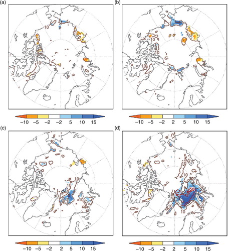
Fig. 1 Colour shading shows regressions of sea ice concentration (SIC, %) in (a) August, (b) September, (c) October, (d) November, on BK SIC time series in November. Shading in all panels also indicates areas with 95 % significance level. Contour lines indicate percentage of explained variance in SIC of the same months for November SIC. Original data from NSIDC.

2. Data and methodology

This investigation uses data from the National Snow and Ice Data Center (NSIDC), NCEP/NCAR Reanalysis (Kalnay et al., 1996) and ECMWF-ORAS4 ocean reanalysis (Balmaseda et al., 2013) for 1979 to 2013. For the variables used, SIC (Cavalieri et al., 1996) and ice motion vectors (Fowler et al., 2013) can be considered as measurements, sea-level pressure (SLP) is reanalysis (assimilated) and the surface heat fluxes are simulated (forecast) variables in the NCEP/NCAR Reanalysis. Our approach here is similar to Ogi and Wallace (2007), Ogi et al. (2008), and Ogi et al. (2010) who studied the impact of atmospheric circulation on summer and early autumn Arctic sea ice loss and anomalies. All analyses are based on detrended data with the 5-year running mean removed. This is in order to minimise the direct effects of global warming on the different components which may affect the conclusions about possible physical relationships. In general, the results are not sensitive to the width of the running mean used. We also repeated the SLP analysis with ERA-INTERIM data and found that the result is almost identical. The BK SIC time series (denoted by tSIC) used in the regression analyses is defined as area-averaged SIC over 0 °–90 °E, 75 °–85 °N (King et al., 2016) in November with the 5-year running mean removed. Shown in Fig. 1d is the spatial pattern associated with November tSIC, while the other panels the preceding 3 months. It is found that there is no strong SIC persistence in these months in the BK seas, which suggests that dynamical effects rather than purely sea ice persistence are at work in determining the SIC anomaly in November.

3. Results

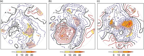
The relationship of low level winds and sea ice motion are likely to be characterised by Ekman drift (Ogi et al., 2008; Ogi and Wallace, 2007). To examine the possible role of the geostrophic winds we calculate the regressions of the mean SLP in August, September and October, respectively on November tSIC (Fig. 2a–c). For October, there is a positive (negative) SIC anomaly in the BK seas that is related to anomalous northerly (southerly) and westerly (easterly) winds through the straits between northern Greenland and Russia. The anomalous cyclonic circulation over the polar area with the associated westerlies over the marginal seas can be responsible for southward Ekman transport of sea ice (Ogi and Wallace, 2007). The correlation coefficients between November tSIC and time series defined by the area average of the negative SLP anomaly (Fig. 2, top row) in the months of October (using 60 °–120 °E,70 °–90 °N), September (using 90 °–150 °E,70 °–80 °N) and August (using 30 °–90 °E,70 °–80 °N) are −0.53, −0.39 and −0.37, respectively. This suggests that, by square of the correlation coefficients, up to 28 % of the November BK SIC variance can be accounted for by SLP in October, but it drops to about 15 % in September and August.

Fig. 2 Contours show regressions of sea-level pressure in (a) August, (b) September, (c) October, on BK SIC time series in November. Contour interval (CI) = 0.3 hPa. Solid (dashed) lines indicate positive (negative) values. Shading indicates percentage of explained variance in SLP as well as areas with 95 % significance level. Original data from NCEP/NCAR Reanalysis and NSIDC.

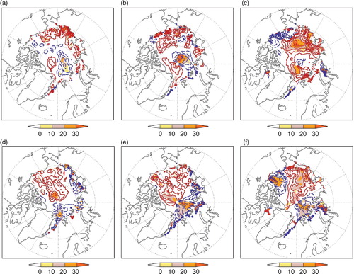
The anomalous wind directions inferred by SLP in Fig. 2 are consistent with the advection of sea ice from the north as well as a colder Arctic air that promotes heat loss from the sea (and thus freezing). Both of these processes encourage SIC increase in a cold season. Next, we examine these two effects. Shown in Fig. 3 are regressions of anomalous sea ice drift velocities on November tSIC. The drift velocity in the zonal and meridional directions is plotted separately because they have different locations of statistical significance. The directions of the anomalous sea ice motion are consistent with the wind-driven effects. In October, positive SIC anomaly in the BK seas is associated with an eastward drift (Fig. 3c, i.e. cyclonic motion) of the whole Arctic sea ice, and a southward export (Fig. 3f), presumably resulted from Ekman transport, of sea ice through the straits of Greenland and Barents seas. However, in September the anomalous sea ice velocities that contribute to the positive BK SIC anomaly in November are resulted from sea ice being pushed directly by the winds towards the straits, from area near the Canadian Arctic coast and the Pole (Fig. 3b and e). This latter sea ice export scenario appears to be similar to the transpolar drift stream of sea ice driven by an atmospheric dipole anomaly identified by Wang et al. (2009) for the summer seasons. However, in the summer a southward sea ice export would contribute to sea ice loss, because the sea ice is being moved to an environment warm enough to melt it (Wang et al., 2009).

Fig. 3 Regressions of sea ice drift velocities (CI=2 cm/s) in August (left), September (middle) and October (right) on BK SIC in November, solid (dashed) lines indicate positive (negative) values. Top row shows zonal drift velocity; bottom row meridional drift velocity. Shading indicates percentage of explained variance in drift velocity, as well as areas with 95 % significance level. Original data from NSIDC.

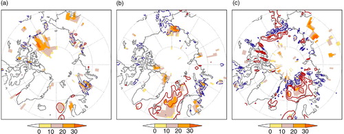
Besides the contribution of sea ice motions, anomalous BK SIC in November also depends on anomalous local sea freezing. To examine this process, regressions of the surface turbulent (sensible and latent; positive upward) heat flux on the November tSIC are calculated (Fig. 4). Heat fluxes at the ocean surface depend on the state of the top ocean layer and the atmosphere. A cold northerly wind anomaly (Fig. 2b) tends to promote the upward turbulent heat flux in the Norwegian Sea in September (Fig. 4b), while cyclonic wind anomaly over the Arctic produce the same for Barents Sea in October (Fig. 4c). The heat release cools the ocean and preconditions it for sea freezing in November. It is found that the explained variances for turbulent heat flux on November BK sea ice anomaly (shading in Fig. 4) are of similar magnitudes to those for SLP and ice drift velocities which top at 30–40 %.

Fig. 4 Regressions of surface turbulent heat flux (CI=5 W/m2, positive upwards) in (a) August, (b) September, and (c) October on BK SIC in November; solid (dashed) lines indicate positive (negative) values. Shading indicates percentage of explained variance in turbulent heat flux, as well as areas with 95 % significance level. Original data from NCEP/NCAR Reanalysis and NSIDC.

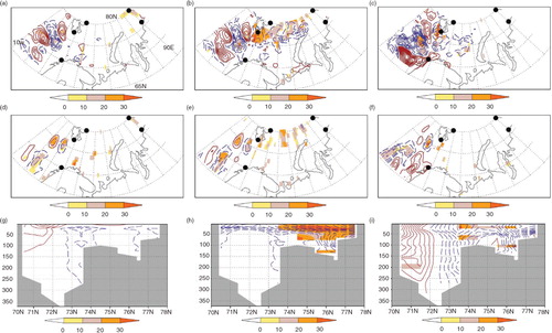
To investigate the role of ocean heat transport, we calculate the regressions of vertically integrated zonal and meridional heat transport on November tSIC (Fig. 5, top and middle rows). The heat transport here is defined as ρc_pTvA (unit=W), where ρ is density, c_p is heat capacity, T is temperature, v is zonal or meridional velocity and A the grid cell area through which the heat transport occurs. The ECMWF-ORAS4 data which have a 1-degree resolution are used here for the ocean variables. The strongest signals appear to be those of the anomalous westward zonal heat transport at 1-month and 2-month leads (Fig. 5b and c), where the highest variance explained is found to be at the Barents Sea Opening (around 20 °E). The regressions of ocean heat flux through the 18.5 °E plane are also shown in Fig. 5 (bottom), which indicate that statistical significant anomalies are found at relatively shallow area of not more than 100 m deep. For the vertically integrated heat transport, the highest amplitude of correlation coefficient with November tSIC is around 0.6, indicating a maximum explained variance of 36 %. The net heat transport into the oceanic region bounded by longitudinal and latitudinal sides between the black dots shown in Fig. 5 is also calculated. It is found that in October and September, the correlations with November tSIC are at −0.6 and −0.55, respectively, while the August heat transport does not provide statistical significant result. The oceanic heat transport thus appears to also account for a high explained variance of November BK SIC. Note that, as for the anomalous surface turbulent heat flux, the ocean heat transport and SLP anomalies may not be totally independent of each other. Our overall results also complement studies on roles of Barents Sea heat transport and high-latitude atmospheric circulations on long-term loss or interannual variation of BK sea ice (e.g. Årthun et al., 2012; Herbaut et al., 2015).

Fig. 5 Regressions of vertically integrated zonal (top), meridional (middle) heat transport at each grid cell (CI=0.5e14 W) on November BK SIC time series. Bottom panel is the same but for zonal heat flux (CI=0.5e6 W/m2) on the 18.5 °E plane. Left, middle and right panels for August, September and October, respectively. Solid (dashed) lines indicate positive (negative) values. Shading indicates percentage of explained variance, as well as areas with 95 % significance level. Original data from ECMWF-ORAS4 and NSIDC.

4. Conclusions

This note provides dynamical interpretation for the statistical relationship between atmospheric circulation anomalies in October and BK SIC in November found previously (Garcia-Serrano et al., 2015; King et al., 2016). Regression analyses show that cyclonic (anticyclonic) wind anomaly over the Arctic in October sets up Ekman drift of sea ice through the Greenland and Barents seas, contributing to positive (negative) SIC anomaly there. In September, however, the contributing factor appears to be a direct export of sea ice through the straits due to an atmospheric dipole anomaly similar to that described by Wang et al. (2009). The transition of the SLP dipolar anomalous atmospheric forcing in September to the monopole anomalous circulation in October (Fig. 2) is not addressed in this study. Further question also remains about the forcing on the SLP anomalies shown. Possible factors include internal atmospheric variability, remote and local sea surface temperature anomalies, and feedback from the sea ice. Future studies investigating these questions will require suitable model experiments as well as observational data analyses. The anomalous northerly (southerly) winds through the straits of Greenland and Barents seas in September and October can also promote (impede) upward surface turbulent heat flux which preconditions the ocean for more (less) freezing in November. Ocean heat transport into the BK seas in the preceding 2 months is also found to contribute to the November SIC anomaly. The anomalous sea ice motions, turbulent heat flux and ocean heat transport in August are not found to have strong relationship with the BK SIC in November. This study adds another important step towards understanding of the lead–lag ice-ocean–atmosphere interactions from the autumn to winter seasons.

5. Acknowledgements

JG-S has been supported by the European Union's FP7-funded NACLIM project (ENV-308299) and H2020-funded DPETNA grant (MSCA-IF-EF 655339). MPK acknowledges the Severo Ochoa Visiting Fellowship at the Barcelona Supercomputing Center and the Nordforsk GREENICE project (61841). Mehmet Ilicak and Marius Årthun provided suggestions related to ocean heat transport. Suggestions from the reviewer had also led to improvement in the analyses.

References

- Årthun M., Eldevik T., Smedsrud L., Skagseth Ø., Ingvaldsen R. Quantifying the influence of Atlantic heat on Barents Sea ice variability and retreat. J. Clim. 2012; 25: 4736–4743. http://dx.doi.org/10.1175/JCLI-D-11-00466.1.
- Balmaseda M. A., Ferranti L., Molteni F., Palmer T. N. Impact of 2007 and 2008 Arctic ice anomalies on the atmospheric circulation: implications for long-range predictions. Q. J. R. Meteorol. Soc. 2010; 136: 1655–1664. http://dx.doi.org/10.1002/qj.661.
- Balmaseda M. A., Mogensen K., Weaver A. T. Evaluation of the ECMWF ocean reanalysis system ORAS4. Q. J. R. Meteorol. Soc. 2013; 139: 1132–1161. http://dx.doi.org/10.1002/qj.2063.
- Cavalieri D. J. , Parkinson C. L. , Gloersen P. , Zwally H . Updated Yearly. Sea Ice Concentration From Nimbus-7 SMMR and DMSP SSM/I-SSMIS Passive Microwave Data. 1996. NASA DAAC at the National Snow and Ice Data Center, Boulder, CO.
- Cohen J., Screen J. A., Furtado J. C., Barlow M., Whittleston D., co-authors. Recent Arctic amplification and extreme mid-latitude weather. Nat. Geosci. 2014; 7: 627–637. http://dx.doi.org/10.1038/NGEO2234.
- Doblas-Reyes F. J., Garcia-Serrano J., Lienert F., Pinto-Biecas A., Rodrigues L. R. L. Seasonal climate predictability and forecasting: status and prospects. WIREs Cim. Change. 2013; 4: 245–268. http://dx.doi.org/10.1002/wcc.217.
- Fereday D. R., Maidens A., Arribas A., Scaife A. A., Knight J. R. Seasonal forecasts of northern hemisphere winter 2009/10. Environ. Res. Lett. 2012; 7: 034031. http://dx.doi.org/10.1088/1748-9326/7/3/034031.
- Fowler C. , Emery W. , Tschudi M . Polar Pathfinder Daily 25 km EASE-Grid Sea Ice Motion Vectors. 2013. Version 2, National Snow and Ice Data Center, Boulder, CO.
- Garcia-Serrano J., Frankignoul C., Gastineau G., de la Camara A. On the predictability of the winter Euro-Atlantic climate: lagged influence of autumn Arctic sea ice. J. Clim. 2015; 28: 5195–5216. http://dx.doi.org/10.1175/JCLI-D-14-00472.1.
- Herbaut C., Houssais M.-N., Close S., Blaizot A.-C. Two wind-driven modes of winter sea ice variability in the Barents Sea. Deep. Sea Res. I. 2015; 106: 97–115. http://dx.doi.org/10.1016/j.dsr.2015.10.005.
- Kalnay E. , Kanamitsu M. , Kistler R. , Collins W. , Deaven D. , co-authors . The NCEP/NCAR 40-year reanalysis project. Bull. Amer. Meteor. Soc. 1996; 77: 437–471.
- King M. P., Hell M., Keenlyside N. Investigation of atmospheric mechanisms related to the autumn sea ice and winter circulation link in the Northern Hemisphere. Clim. Dyn. 2016; 46: 1185–1195. http://dx.doi.org/10.1007/s00382-015-2639-5.
- Nakamura T., Yamazaki K., Iwamoto K., Honda M., Miyoshi Y., co-authors. A negative phase shift of the winter AO/NAO due to the recent Arctic sea-ice reduction in late autumn. J. Geophys. Res. Atmos. 2015; 120: 3209–3227. http://dx.doi.org/10.1002/2014JD022848.
- Ogi M., Rigor I. G., McPhee M. G., Wallace J. M. Summer retreat of Arctic sea ice: role of summer winds. Geophys. Res. Lett. 2008; 35: 24701. http://dx.doi.org/10.1029/2008GL035672.
- Ogi M., Wallace J. M. Summer minimum Arctic sea ice extent and the associated summer atmospheric circulation. Geophys. Res. Lett. 2007; 34: 12705. http://dx.doi.org/10.1029/2007GL029897.
- Ogi M., Yamazaki K., Wallace J. M. Influence of winter and summer surface wind anomalies on summer Arctic sea ice extent. Geophys. Res. Lett. 2010; 37: 07701. http://dx.doi.org/10.1029/2009GL042356.
- Orsolini Y. J., Senan R., Benestad R. E., Melsom A. Autumn atmospheric response to the 2007 low Arctic sea ice extent in coupled ocean–atmosphere hindcasts. Clim. Dyn. 2012; 38: 2437–2448. http://dx.doi.org/10.1007/s00382-011-1169-z.
- Riddle E. E., Butler A. H., Furtado J. C., Cohen J. L., Kumar A. CFSv2 ensemble prediction of the wintertime Arctic Oscillation. Clim. Dyn. 2013; 41: 1099–1116. http://dx.doi.org/10.1007/s00382-013-1850-5.
- Scaife A. A., Arribas A., Blockley E., Brookshaw A., Clark R. T., co-authors. Skillful long-range of European and North American winters. Geophys. Res. Lett. 2014; 41: 2514–2515. http://dx.doi.org/10.1002/2014GL059637.
- Stockdale T. N., Molteni F., Ferranti L. Atmospheric initial conditions and the predictability of the Arctic Oscillation. Geophys. Res. Lett. 2015; 42: 1173–1179. http://dx.doi.org/10.1002/2014GL062681.
- Sun L., Deser C., Tomas R. A. Mechanisms of stratospheric and tropospheric circulation response to projected Arctic sea ice loss. J. Clim. 2015; 28: 7824–7845. http://dx.doi.org/10.1175/JCLI-D-15-0169.1.
- Wang J., Zhang J., Watanabe E., Ikeda M., Mizobata K., co-authors. Is the dipole anomaly a major driver to record lows in Arctic summer sea ice extent?. Geophys. Res. Lett. 2009; 36: 05706. http://dx.doi.org/10.1029/2008GL036706.