Decadal predictability of regional scale wind speed and wind energy potentials over Central Europe

Abstract

Decadal predictions on timescales from one year to one decade are gaining importance since this time frame falls within the planning horizon of politics, economy and society. The present study examines the decadal predictability of regional wind speed and wind energy potentials in three generations of the MiKlip (‘Mittelfristige Klimaprognosen’) decadal prediction system. The system is based on the global Max-Planck-Institute Earth System Model (MPI-ESM), and the three generations differ primarily in the ocean initialisation. Ensembles of uninitialised historical and yearly initialised hindcast experiments are used to assess the forecast skill for 10 m wind speeds and wind energy output (Eout) over Central Europe with lead times from one year to one decade. With this aim, a statistical-dynamical downscaling (SDD) approach is used for the regionalisation. Its added value is evaluated by comparison of skill scores for MPI-ESM large-scale wind speeds and SDD-simulated regional wind speeds. All three MPI-ESM ensemble generations show some forecast skill for annual mean wind speed and Eout over Central Europe on yearly and multi-yearly time scales. This forecast skill is mostly limited to the first years after initialisation. Differences between the three ensemble generations are generally small. The regionalisation preserves and sometimes increases the forecast skills of the global runs but results depend on lead time and ensemble generation. Moreover, regionalisation often improves the ensemble spread. Seasonal Eout skills are generally lower than for annual means. Skill scores are lowest during summer and persist longest in autumn. A large-scale westerly weather type with strong pressure gradients over Central Europe is identified as potential source of the skill for wind energy potentials, showing a similar forecast skill and a high correlation with Eout anomalies. These results are promising towards the establishment of a decadal prediction system for wind energy applications over Central Europe.

• decadal prediction
• regionalisation
• wind speed
• wind energy
• Central Europe
• statistical-dynamical downscaling
• MiKlip decadal prediction system
• MPI-ESM
• COSMO-CLM

To access the supplementary material to this article, please see Supplementary files under ‘Article Tools’.

1. Introduction

The demand for renewable, ecologically sustainable energy sources as alternative to fossil sources has strongly increased in recent years (Solomon et al., 2007). In Europe, wind energy production has emerged as a promising renewable energy source to face the projected climate change due to increasing greenhouse gas emissions. The currently installed wind energy capacity in Europe has the potential to produce enough electricity to cover up to 8 % of the EU's electricity demand (Pineda et al., 2014). By 2020, the European Commission aims to produce 14.9 % of the EU's electricity from wind energy resources (Moccia et al., 2014). Wind energy production itself is influenced by weather and climate due to its dependence on near-surface wind conditions (e.g. Pryor and Barthelmie, 2010). In recent years, several studies investigated the impact of climate change on wind speeds and wind energy production over Europe on the regional scale for the middle and end of the 21st century (e.g. Barstad et al., 2012; Pryor et al., 2012; Hueging et al., 2013; Tobin et al., 2014; Reyers et al., 2016). These studies used different global and regional climate models (GCMs and RCMs) with different emission scenarios and downscaling techniques, and focused on different parts of Europe. Most of these studies agree on a general increase in wind energy potentials over Northern Europe and a general decrease over Southern Europe in future decades. Differences can be found regarding the magnitude and sometimes the sign of the projected changes. These differences seem to result not only from different initial conditions and model parameterisations but also from downscaling technique (e.g. Pryor et al., 2005, 2012; Tobin et al., 2014; Reyers et al., 2016). However, both potential long-term trends and future changes for wind speed and wind energy potentials are quite small compared to temperature trends (IPCC, 2012). At the same time, the natural variability of wind, especially on interannual to decadal timescales, is quite large and might conceal potential long-term trends.

Short-term climate predictions, which can assess this decadal variability, are of particular interest for the development of wind energy production, as their time frame of one year up to one decade falls within the planning horizon of politics and economy (e.g. Meehl et al., 2009). The German consortium MiKlip (‘Mittelfristige Klimaprognosen’, decadal climate predictions; Marotzke et al., submitted) developed a model system based on the Max-Planck-Institute Earth System Model (MPI-ESM) to provide skilful decadal predictions on global and regional scales. Therefore, the decadal predictions should represent natural variability as well as changes due to increasing greenhouse gas emissions (e.g. Solomon et al., 2011). The present study evaluates several generations of the MPI-ESM decadal prediction system recently conducted within MiKlip with respect to the decadal predictability of regional wind speed and wind energy production. The first generation of MPI-ESM decadal predictions (baseline0) contributes to the Coupled Model Intercomparison Project Phase 5 (CMIP5; Taylor et al., 2012). An overview over recent studies, especially from CMIP5, and the current state-of-the-art for decadal predictions can be found in Meehl et al. (2014). Through CMIP5, a set of global decadal hindcast experiments (initialised forecasts of past cases) and predictions (of future cases) has been made available. The initial conditions for these decadal runs are taken from assimilation runs, which use reanalysis data (ocean-only or ocean-atmosphere) from the past and the present (see Section 2.1). Ensembles are generated by initialising the simulations at different time steps of the assimilation run (usually 1-day-lagged initialisation; e.g. Müller et al., 2012). The hindcast experiments are used to analyse the decadal predictability for different parameters through a comparison to observations and reanalysis data (e.g. Smith et al., 2007).

Several publications assessed the decadal forecast skill of existing forecast systems, either for individual model ensembles (e.g. Müller et al., 2012, 2014; Goddard et al., 2013; Marotzke et al., submitted) or for multi-model ensembles (e.g. van Oldenborgh et al., 2012; Doblas-Reyes et al., 2013; Eade et al., 2014). Most of these studies focus on the global scale and on primary meteorological parameters like temperature (e.g. Smith et al., 2007; Müller et al., 2012) and precipitation (e.g. van Oldenborgh et al., 2012). Although all of these studies found some decadal forecast skill, their results differ for different parameters, regions and lead times. In particular, Eade et al. (2014) indicated that potential skill in decadal prediction systems may often be underestimated. Nevertheless, most of them agree that the North Atlantic is a key region for decadal climate predictions (e.g. Müller et al., 2012). So far, only few studies investigated decadal predictions on the regional scale, and to our knowledge, none is dealing with wind energy. Kruschke et al. (2014), for example, analysed the decadal forecast skill for cyclone activity over the Northern Hemisphere in the MPI-ESM and found some regions over the North Atlantic with positive predictive skill for intense cyclones. Mieruch et al. (2014) investigated the decadal forecast skill for seasonal temperature anomalies and precipitation sums in dynamically downscaled MPI-ESM hindcasts, focusing on Europe. They found a good predictive skill for summer temperature, which could be preserved by regionalisation. Predictive skill for precipitation sums could even be improved by the downscaling in their study. Haas et al. (2015) evaluated the decadal predictability of peak winds on the regional scale in the MPI-ESM, using a statistical-dynamical downscaling (SDD) approach for the regionalisation. Their results showed highest skill scores for short lead times and upper gust percentiles.

For the application to regional scales, the resolution of the global decadal predictions is insufficient. Therefore, a downscaling of the global datasets to the regional scale is necessary (e.g. Mieruch et al., 2014; Haas et al., 2015). In principle, it is possible to use a dynamical downscaling (DD) approach for the regionalisation of large ensembles, depending on available computing power, storage capacities and time. However, since most decadal prediction systems comprise multiple ensemble members of yearly initialised hindcasts, resulting in a total of several hundreds of simulations per ensemble generation (see Section 2.1), it is hardly possible to regionalise the entire hindcast ensemble using a purely DD method. The present study uses a SDD approach (following Fuentes and Heimann, 2000; Pinto et al., 2010) to investigate the decadal predictability of wind energy potentials over Central Europe, with special focus on Germany. SDD approaches combine a purely DD application with statistical approaches, for example weather type analysis (e.g. Reyers et al., 2015) or transfer functions (e.g. Najac et al., 2011; Haas and Pinto, 2012). This combination offers a good and cost-efficient alternative to DD. In this study, we applied the SDD approach developed by Reyers et al. (2015) to the decadal hindcasts and predictions of the MPI-ESM and analysed the decadal forecast skill for different lead times and different seasons. The focus of this study is given to wind and wind energy potentials over Germany.

The paper is organised as follows. The decadal prediction and hindcast datasets are described in Section 2 (part 2.1). Additionally, Section 2 contains the methodology of SDD (2.2), bias and drift correction (2.3), and an explanation of the skill metrics (2.4). The results for wind speed are presented in Section 3: the added value of downscaling is addressed in Section 3.1, while Section 3.2 contains the forecast skill for different wind percentiles. The results for wind energy potentials are described in Section 4, focusing on the forecast skill over Central Europe (4.1), the seasonal dependence of forecast skill (4.2) and a potential source of forecast skill (4.3). A short summary and discussion of the results concludes this paper in Section 5.

2. Data and methods

2.1. Data

Three decadal prediction generations of the coupled model MPI-ESM performed in low-resolution mode (MPI-ESM-LR; Giorgetta et al., 2013) are analysed. The coupled model consists of the atmospheric model ECHAM6 (Stevens et al., 2013), the ocean model MPIOM (Jungclaus et al., 2013), the land-biosphere model JSBACH (Raddatz et al., 2007) and the ocean-biogeochemistry model HAMOCC (Ilyina et al., 2013), coupled by OASIS3 (Valcke et al., 2003). The atmospheric component is run with a T63 horizontal resolution (1.875°) and 47 vertical levels, and the MPIOM with a horizontal resolution of 1.5° and 40 vertical levels.

The three MPI-ESM ensemble generations differ in their initialisation (see Table 1; cf. also Marotzke et al., submitted). The first analysed generation of decadal hindcasts is called baseline1 (second MiKlip ensemble generation). The initial conditions are taken from an assimilation experiment, where the model state is nudged towards ocean temperature and salinity anomalies of an MPIOM experiment forced with ORA-S4 ocean reanalysis (Balmaseda et al., 2013), and full atmospheric fields from ERA40 (Uppala et al., 2005) and ERA-Interim (Dee et al., 2011). The baseline1 ensemble consists of 10 members of yearly initialised decadal hindcasts and predictions from the initialisation year 1960 (hereafter dec1960: comprising the 10-yr period 01 January 1961 to 31 December 1970) to 2011 (dec2011: comprising the 10-yr period 01 January 2012 to 31 December 2021), and is described in detail in Pohlmann et al. (2013). The latest MPI-ESM generation – named prototype – differs from baseline1 in terms of full-field ocean initialisation and consists of two separate ensembles (see Table 1). The first prototype ensemble (hereafter prototype1) uses full-fields from ORA-S4 reanalysis, while the second prototype ensemble (hereafter prototype2) uses full-fields of GECCO2 ocean reanalysis (Köhl, 2015). Both prototype1 and prototype2 ensembles consist of 15 members of yearly initialised decadal hindcasts and predictions, from which 10 members are utilised here for the initialisation period 1960–2013 (dec1960 to dec2013). For all three generations, the ensemble members are generated through a 1-day-lagged initialisation (e.g. Müller et al., 2012). Further, uninitialised historical runs are used here as reference datasets to estimate the added value of initialisation (see also Section 2.4). They consist of 10 ensemble members and are started from a pre-industrial control simulation and consider aerosol and greenhouse gas concentrations for the period 1850–2005 (e.g. Müller et al., 2012). The first MiKlip ensemble generation baseline0 is not discussed here due to the limited number of runs (10 members every 5 yr for the period 1960–1999, 10 members for the period 2000–2010 and only three members in every other year).

Table 1. Overview of the three MPI-ESM ensemble generations used in this study, including information on the name within the MiKlip consortium, the ocean initialisation, the atmosphere initialisation and the number of ensemble members.

Ensemble	Ocean initialisation	Atmosphere initialisation	# Ensemble member
baseline1	Anomalies from ORA-S4 reanalysis	Full-fields from ERA-Interim/ERA40	10
prototype1	Full-fields from ORA-S4 reanalysis	As above	10 (from 15)
prototype2	Full-fields from GECCO2 reanalysis	As above	10 (from 15)
historical	–	–	10 (from 15)

In order to enable a direct comparison between the different ensembles, 10 simulations are used for all datasets. All simulations correspond to the ‘low-resolution’ set up.

To evaluate the model performance in terms of the decadal forecast skill, observations or reanalysis datasets are usually used. In this study, we consider the ERA-Interim reanalysis dataset (Dee et al., 2011) for evaluation and for the computation of different forecast skill scores (see also Section 2.4). ERA-Interim is the third global reanalysis dataset of the European Centre for Medium-Range Weather Forecasts (ECMWF). It is available from 1979 onwards. In this study, we use ERA-Interim data for the period 1979–2010.

2.2. Statistical-dynamical downscaling methodology

We follow the SDD methodology by Reyers et al. (2015) to downscale the global MPI-ESM hindcasts and historical runs to derive regional wind speeds and wind energy production. Since the SDD approach for the application to wind energy potentials is described in detail in Reyers et al. (2015), only a short summary is given here. SDD consists of four steps:

In the first step, a circulation weather type (CWT) approach after Jones et al. (1993) is applied to daily mean sea level pressure (MSLP) fields, using the following global datasets as input data: ERA-Interim reanalysis for evaluation, 10 historical runs and three ensembles of MPI-ESM hindcasts for the analysis of decadal predictability. All datasets are interpolated on the same regular 2.5° grid for the computation of the CWTs. The large-scale atmospheric flow as represented by the instantaneous MSLP fields is characterised for each day for Central Europe using the central point at 10°E, 50°N (near Frankfurt, Germany; Fig. 1a). The patterns are assigned to 10 basic CWTs (eight directional and two rotational classes; e.g. west W or cyclonic C) and one mixed CWT (anti-cyclonic/west AW). The days corresponding to the AW type are not accounted for in the basic A or W types. In addition, the 11 CWTs are subdivided into classes with different pressure gradients in 5 hPa per 1000 km intervals, ranging from below 5 hPa per 1000 km to ca. 45 hPa per 1000 km. Altogether, 77 weather classes are considered.

Fig. 1 (a) Topography of Europe in metre, and grid points for CWT analysis (step 1 of SDD). The red point represents the central point at 10°E, 50°N (near Frankfurt, Germany), and the red crosses represent the surrounding 16 grid points used for the computation of the CWTs. The white box represents the region for figures (b) to (d). (b) Climatological mean of mean 10 m wind speed in metre per second for ERA-Interim (1979–2010) as obtained by SDD. (c) Climatological mean of annual Eout in 10³ MWh for ERA-Interim (1979–2010) as obtained by SDD. (d) Explained variance between annual Eout time series for ERA-Interim (1979–2010) as obtained by SDD and as obtained by DD (DD_era) per CCLM grid point. Grid points with significant correlation are dotted (t-test, 95% confidence level). Box 1 represents the subregion for the computation of the MSE skill scores as shown in Fig. 5 and Supplementary Figs. 2–5 (see also Section 4), and box 2 represents the subregion for the averages over Germany (7°E–14°E, 48°N–53°N) as shown in Figs. 2, 3, 4, Figs. 6, 7 and Supplementary Fig. 1.

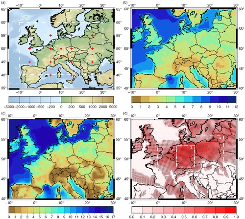
In the second step, representative days for each of the 77 classes are simulated with the regional climate model COSMO of the German Weather Service (Deutscher Wetterdienst, DWD) in its Climate Mode (version 4.8, hereafter CCLM; e.g. Rockel et al., 2008). CCLM simulations with a horizontal resolution of 0.22° are performed for the model domain of the EURO-CORDEX project (Giorgi et al., 2006), using ERA-Interim data as initial and boundary conditions. For each of the 77 weather classes, up to 10 representatives have been extracted. Note that the ERA-Interim-driven representatives are used for the regionalisation of all global datasets, assuming that the wind characteristics of the different CWTs are similar in both the model and the reanalysis (see Reyers et al., 2015).

In the third step, simulated hourly 10 m wind speeds of the representative days are recombined to probability density functions (PDFs) at each CCLM grid point. Therefore, we weighted the contributions of all 77 classes by the respective class frequency (e.g. frequency of a weather class in a certain decade) and the number of representative days.

The last step is subdivided into two separate substeps, one for wind speed and one for wind energy potentials. For wind speed, the PDFs of the hourly 10 m wind speeds are directly used to calculate different wind percentiles and the mean wind for each grid point. Figure 1b shows the spatial distribution of the mean wind for ERA-Interim (climatology for 1979–2010) as obtained by SDD. For wind energy applications, the PDFs of the hourly 10 m wind speeds are used to calculate gridded wind energy output (Eout) of a 2.5-MW wind turbine from General Electrics (2010). First, the hourly 10 m wind speeds are extrapolated to the average turbine hub height using a vertical wind profile, which is the standard procedure in wind energy applications from the ‘large-scale’ perspective (e.g. Hueging et al., 2013; Tobin et al., 2014). Here, the power law is used to extrapolate the 10 m wind speeds to a height of 80 m (v80; Reyers et al., 2015). The extrapolated wind speeds form the basis to compute Eout, following these characteristics: Below v80=3.5 m/s (cut-in velocity) and above v80=25 m/s (cut-out velocity), no energy output is produced. Between the cut-in velocity (3.5 m/s) and the rated velocity (12.5 m/s), Eout is calculated as:1

with power coefficient c _p (constant value of 0.35 for the idealised turbine), air density ρ (constant value of 1.225 kg m⁻³) and rotor radius R of the idealised wind turbine (50 m). Between wind velocities of 12.5 m/s (rated velocity) and 25 m/s (cut-out velocity), a constant maximum Eout of 2.5 MW is assumed. To obtain spatial distributions of mean annual wind energy output for each CCLM grid point, Eout is integrated over all wind speed ranges and weighted with the respective climatological velocity frequencies. Figure 1c shows the spatial distribution of mean annual Eout for the ERA-Interim data (climatology for 1979–2010) as obtained by SDD. For the application of SDD to the different MPI-ESM datasets and to different time periods, only the weather type computation (step 1) has to be recalculated.

Reyers et al. (2015) evaluated the results for the SDD approach for wind energy potentials against a purely DD method applied to ERA-Interim. The results show a good agreement for Central Europe (see also Fig. 1d; explained variance between annual Eout as obtained by SDD and annual Eout as obtained by DD), while agreement is reduced over other areas, like the North Sea or the Mediterranean region. They also tested the applicability of SDD to decadal hindcasts of the baseline1 ensemble and concluded that SDD performs well for Germany, the Benelux region, the Czech Republic, and Poland (cf. Reyers et al., 2015; their figures 10 and 11). The lower performance of the SDD approach in other European countries is due to the considered CWT classification, which is centred over Germany and thus has a better performance over Germany and nearby countries (see Fig. 1a; Reyers et al., 2015).

2.3. Bias and potential drift correction

Several studies revealed a systematic bias in the MPI-ESM historical runs and hindcasts due to model drifts (e.g. Kruschke et al., 2014, 2015). This systematic bias is both dependent on the model generation and forecast time. The International CLIVAR Project Office (ICPO; 2011) suggests a bias correction for anomaly-initialised predictions and uninitialised simulations by subtracting a climatological bias, while a subtraction of lead time-dependent bias should be used for full-field initialised predictions. In a sensitivity study, we applied a bias correction to the CWT frequencies of the baseline1 ensemble (first step of the SDD; see Section 2.2). In terms of our SDD approach, the systematic bias is reflected by an overestimation of the frequencies of some weather types, especially the westerly types over Europe (see Reyers et al., 2016; their table 2 and figure 1b). This is due to the typical overestimation of the zonal flow in the North Atlantic/European Sector in GCMs (e.g. Sillmann and Croci-Maspoli, 2009). Therefore, the climatological CWT frequencies for both decadal hindcasts and uninitialised historical runs were corrected towards the respective climatological frequencies of ERA-Interim. The resulting empirical factors have been applied to the decadal CWT frequencies for the different lead times, which were then used for the computation of Eout. However, since the bias is systematic in CWT frequencies of both hindcasts and the historical runs as reference dataset, the bias correction has only negligible effects on our results (not shown).

Kharin et al. (2012) stated that it is problematic to assume a constant model drift, especially when differences between observed and modelled long-term climate trends are large. This is in particular the case for decadal predictions initialised by full-fields (e.g. prototype). We also analysed the potential model drift in the prototype1 ensemble, focusing on CWT frequencies and 10 m wind speeds. In both cases, the consequences of the model drift are small for our approach (not shown). Therefore, we have chosen to use the original datasets for all analyses.

2.4. Forecast skill assessment

Three different metrics are used to identify a potential added value of downscaling and estimate whether the initialisation of the hindcasts improves the decadal predictability compared to the uninitialised historical runs: the mean square error skill score (MSESS) and the ranked probability skill score (RPSS) to quantify the accuracy of the hindcasts, and the reliability (REL) to assess the relation between ensemble spread and bias. The different skill metrics are calculated for seven different lead times for the whole year and the single seasons. Lead times corresponding to the first half of the decade (e.g. yr1-3: first to third year after initialisation; hereafter short lead times) represent skill that is supposed to originate from the initialisation. We also considered lead times corresponding to the second half of the decade (e.g. yr6-9: sixth to ninth year after initialisation; hereafter longer lead times) to see how far ahead the initialisation provides predictive skill. Moreover, one lead time covering nearly the whole decade (yr2-9) is analysed. As suggested by Goddard et al. (2013), lead times are temporally averaged. All three skill metrics compare the MPI-ESM ensembles to observations. Since no gridded observations for wind are available for Central Europe, we used a purely DD simulation of a reanalysis dataset instead as verification dataset. DD is simulated with CCLM, using ERA-Interim data for 1979–2010 as boundary conditions (hereafter DD_era; see Reyers et al., 2015). As DD_era is available for the period 1979–2010, we decided to use the decadal hindcasts dec1978 (1979–1988) to dec2000 (2001–2010) for the computation of the metrics in this study. Thereby, we ensure that the same number of yearly initialised hindcasts is considered for all lead times. The study focuses on Central Europe (box 1 in Fig. 1d) and Germany (box 2 in Fig. 1d; 7°–14°E and 48°–53°N), since the results of the CWT approach are primarily representative for the large-scale atmospheric conditions over Germany and surrounding countries (cf. Fig. 1d and Reyers et al., 2015). Temporal anomalies are used for the computations of the skill metrics rather than absolute values to remove systematic climatological biases. For Germany, anomalies are spatially averaged before computing the skill scores.

The MSESS (Goddard et al., 2013) is a deterministic skill score and defined as2

where MSE _dec is the mean squared error (MSE) between the ensemble mean of the initialised hindcast experiments and the verification dataset (DD_era). MSE _hist is the MSE of a reference dataset, which is in this case the ensemble mean of the uninitialised historical runs. Therefore, a positive MSESS suggests that the initialised hindcasts are more accurate in representing the observed decadal climate variability than the uninitialised historical runs (Goddard et al., 2013), and a negative value indicates the opposite.

The probabilistic RPSS (Wilks, 2011; Kruschke et al., 2014) is defined as3

where RPS _dec is the ranked probability score (RPS) of the initialised hindcast experiments, and RPS _hist is the RPS of the uninitialised historical runs. The RPS is an extension of the Brier score (scalar accuracy measure for binary events) to multi-category forecasts (Wilks, 2011). Following Kruschke et al. (2014), three categories are used here for the calculation of RPS: below normal, normal and above normal. The categories are defined using the 33.3 and 66.6 percentiles of Eout and wind speed anomaly time series. The RPS is based on the cumulative probabilities for the three categories (Wilks, 2011):4

F _τ,i,k is the cumulative probability of the 10 ensemble members within category k (here K=3), derived from the forecast ensemble of initialisation i (with a total number of I=23, for dec1978–dec2000) for a certain lead time τ. O _t(i,τ),k is the cumulative probability within category k derived from observations (here DD_era) for time t, which corresponds to the time of initialisation i and the lead time τ. O _t(i,τ),k is the Heaviside step function with O _t(i,τ),k =1 if the event occurs in category k or lower or else O _t(i,τ),k =0 if a category higher than k is observed. A positive RPSS therefore indicates that the initialised hindcasts have a higher probability to predict an observed anomaly category than the uninitialised historical runs, and vice versa for a negative RPSS. Following Kruschke et al. (2014), we corrected the RPS for biases due to finite ensemble sizes (see also Ferro, 2007). RPSSs are calculated for different wind percentiles as well as for Eout.

The reliability (REL; Weigel et al., 2009) is defined as5

where RMSE _dec is the root mean square error between the ensemble mean of the initialised hindcasts and the verification dataset DD_era, and is the time-mean ensemble spread. The reliability quantifies if the ensemble spread is able to cover the model uncertainties (Mieruch et al., 2014). The ensemble is well calibrated for REL values around zero. The ensemble is called underconfident if REL<0, and overconfident if REL>0.

3. Decadal predictability of wind speed

3.1. The added value of downscaling

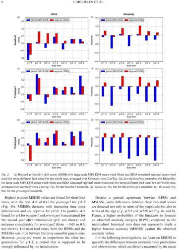
We first analyse the added value of downscaling by comparing large-scale MPI-ESM wind speed to SDD-simulated regional wind speed. With this aim, we calculate skill metrics for both variables. Figure 2 shows the RPSS and the reliability for annual wind speeds averaged over Germany (see box 2 in Fig. 1d) for the three ensemble generations (baseline1, prototype1 and prototype2). All generations exhibit forecast skill, both for large-scale and regional scale wind speeds. The RPSSs are positive for most lead times, with highest skill scores for short lead times (e.g. yr1-3). The regionalisation is able to preserve the decadal forecast skill of the global runs for almost all lead times and in all three ensembles. For some lead times, the downscaling increases the predictive skill. This added value of downscaling is particularly apparent for baseline1 (e.g. yr1-3, yr4-6). Improvements are smaller for the prototype ensembles. The reliability indicates that the global hindcasts are highly underconfident, in particular prototype2. An analysis of the individual components of the reliability [ensemble spread and RMSE, see eq. (5)] reveals that for nearly all lead times the ensemble spread of the global hindcasts clearly exceeds the RMSE (cf. Supplementary Fig. 1). The regionalisation improves both the ensemble spread and the RMSE for most lead times and in all three generations. Since the relative reduction of the spread is larger than that of the RMSE, the two values are now much closer to each other (Supplementary Fig. 1). As a consequence, the SDD ensembles are nearly well calibrated for short lead times in baseline1 and prototype1 and all lead times in prototype2. In summary, an added value of downscaling for wind speed can be identified in the ensemble generations. This added value depends on the lead time and the initialisation.

Fig. 2 (a) Ranked probability skill scores (RPSSs) for large-scale MPI-ESM mean wind (blue) and SDD-simulated regional mean wind (red) for seven different lead times for the whole year, averaged over Germany (box 2 in Fig. 1d), for the baseline1 ensemble. (b) Reliability for large-scale MPI-ESM mean wind (blue) and SDD-simulated regional mean wind (red) for seven different lead times for the whole year, averaged over Germany (box 2 in Fig. 1d), for the baseline1 ensemble. (c)–(d) as (a)–(b), but for the prototype1 ensemble. (e)–(f) as (a)–(b), but for the prototype2 ensemble.

3.2. Forecast skill for different wind percentiles

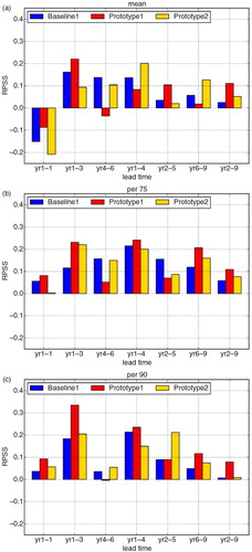
After identifying the added value of our downscaling approach, we focus on the decadal predictability of regional wind speeds. RPSSs are derived for three different percentiles averaged over Germany: mean wind, 75th percentile and 90th percentile (Fig. 3). Positive skill scores are found for all lead times in all three ensemble generations, except for yr1 (first year after initialisation) for mean wind speed (Fig. 3a). Skill scores are highest for short lead times (yr1-3 and yr1-4), with the best skill of 0.34 for prototype1 for yr1-3 for the 90th percentile (Fig. 3c). In this case, the initialisation improves the performance of the decadal prediction system against the uninitialised historical runs by 34 %. Skill scores decrease with increasing time after the initialisation (longer lead times) and are often enhanced for higher percentiles. Differences between the three ensembles are rather small, revealing that no initialisation is clearly superior to the other. Overall, the positive skill scores indicate that the hindcasts are closer to the verification dataset DD_era than the uninitialised historical runs. This is valid not only for the mean wind speed but also for higher percentiles, which are in particular relevant for the wind energy potentials.

Fig. 3 RPSSs for SDD-simulated wind speed for seven different lead times for the whole year, averaged over Germany (box 2 in Fig. 1d), for the ensemble generations baseline1 (blue), prototype1 (red) and prototype2 (yellow), for different percentiles: (a) mean wind, (b) 75th percentile and (c) 90th percentile.

4. Decadal predictability of wind energy potentials

In this section, we assess the decadal predictability of wind energy potentials on the regional scale. Therefore, we first derive forecast skill scores for wind energy output and compare them to skill scores for regional wind speed (Section 4.1). Further, the seasonal dependency of the forecast accuracy is investigated (Section 4.2). Finally, we evaluate potential large-scale sources of forecast skill for wind energy potentials (Section 4.3).

4.1. Forecast skill for Germany and Central Europe

First, RPSSs and MSESSs are calculated for annual Eout anomalies averaged over Germany for seven different lead times. The RPSSs for Eout (Fig. 4a) are analogue to the RPSSs for mean wind speed (cf. Fig. 3a): skill scores are positive for almost all lead times in all three ensembles, highest skill scores are found for short lead times (with the highest value of 0.28 for prototype1 and yr1-3), and skill scores decrease slightly with increasing time since initialisation. However, the forecast skill for Eout and mean wind speed may differ, which is particularly true for longer lead times. This indicates that the decadal predictability of the wind energy output depends on a wider wind speed range, and particularly on the higher percentiles (see Section 3.2).

Fig. 4 Forecast skill scores for SDD-simulated Eout for seven different lead times for the whole year, averaged over Germany (box 2 in Fig. 1d), for the ensemble generations baseline1 (blue), prototype1 (red) and prototype2 (yellow). (a) RPSSs and (b) mean square error skill scores (MSESSs).

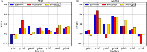
Highest positive MSESS values are found for short lead times, with the best skill of 0.47 for prototype1 for yr1-3 (Fig. 4b). MSESSs decrease with increasing time since initialisation and are negative for yr2-9. The positive skill found for yr1 for baseline1 and prototype1 is maintained for the second year after initialisation (yr2; not shown) and increases considerably for prototype2 (from −0.03 to 0.3; not shown). For most lead times, both the RPSSs and the MSESSs vary little between the three ensemble generations. However, prototype1 seems to outperform the other two generations for yr1-3, a period that is supposed to be strongly influenced by the initialisation.

Despite a general agreement between RPSSs and MSESSs, some differences between these two skill scores are detected not only in terms of the magnitude but also in terms of the sign (e.g. yr2-5 and yr2-9; see Fig. 4a and b). Hence, a higher probability of the hindcasts to forecast an observed anomaly category (RPSS) compared to the uninitialised historical runs does not necessarily imply a higher forecast accuracy (MSESS) against the observed anomaly values.

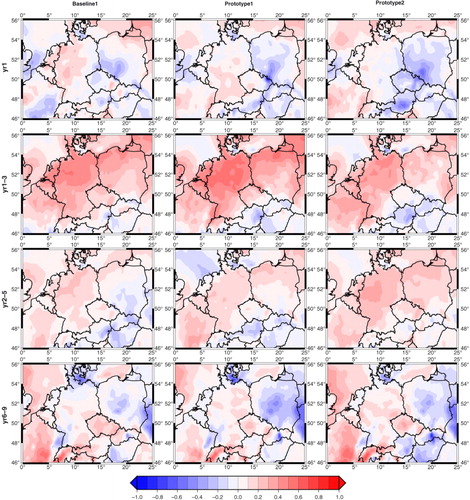
For the following investigations, we focus on MSESS to quantify the differences between ensemble mean predictions and observations, which are directly measured by the mean square error (see Section 2.4). The spatial distributions of MSESS over Central Europe for the annual mean wind energy output are shown in Fig. 5. The three MPI-ESM ensembles are compared for the four exemplary lead times yr1, yr1-3, yr2-5 and yr6-9. Generally, MSESS reveals highest positive values over Northern and Western Germany and the Benelux countries. Differences between the three ensembles are rather small. For yr1 (first year after initialisation), all three ensemble generations show positive skill scores of up to 0.25 for the Benelux countries and large parts of Germany. In these regions, the initialisation of the hindcasts improves their performance against the uninitialised historical runs by 25 %. Negative skill scores of up to −0.5 cover most parts of Poland, the Czech Republic and Eastern Germany, especially for prototype2. For yr1-3 and yr2-5, all three generations show similar distributions of MSESS. For yr1-3, the ensembles show positive skill scores of up to 0.6 over most parts of Central Europe. Skill scores are highest for prototype1 over Germany. For yr2-5, skill scores decline in all three ensembles. They now range from −0.2 (over parts of Poland and the Czech Republic) to 0.4 (over Germany), with highest positive values for prototype2. For yr6-9, skill scores are smallest compared to the other lead times (−0.5 to 0.3).

Fig. 5 MSESSs for SDD-simulated Eout for four exemplary lead times for the whole year for the ensemble generations baseline1 (left column), prototype1 (middle column) and prototype2 (right column). Reference forecast is the ensemble mean of the uninitialised historical runs.

In summary, the three MPI-ESM ensemble generations show an added value of the initialisation compared to the uninitialised simulations and therefore a decadal forecast skill for wind energy output. However, this skill is mostly limited to the first years after initialisation and seems to depend slightly on the initialisation of the different ensemble generations.

4.2. Seasonal dependency of forecast skill

Previous studies (e.g. Müller et al., 2012; Mieruch et al., 2014) found a seasonal dependence of forecast skill in the MPI-ESM in terms of temperature and/or precipitation. Given the strong seasonal variations in wind speed, we calculated MSESSs and RPSSs for Eout for different multi-year seasonal means (Fig. 6 and Supplementary Figs. 2–5 in the appendix).

Fig. 6 MSESSs (left column) and RPSSs (right column) for SDD-simulated Eout for seven different lead times for the four seasons, averaged over Germany (box 2 in Fig. 1d), for the ensemble generations baseline1 (blue), prototype1 (red) and prototype2 (yellow). (a) and (b) Winter (DJF), (c) and (d) spring (MAM), (e) and (f) summer (JJA), (g) and (h) autumn (SON). MSESS values under −1.0 are displayed in the corresponding bar. Note that yr1 for winter corresponds to months 12–14 after initialisation.

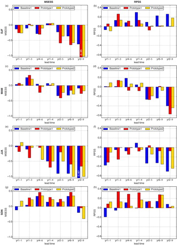
For winter (DJF) means, MSESSs are much weaker than for annual means for all three generations and all lead years. Negative values are found over Germany, the Benelux region, and most parts of Poland and the Czech Republic for almost all lead times (Fig. 6a and Supplementary Fig. 2). MSESS values around zero are only found for short lead times (yr1-3 and yr1-4). As for annual Eout, the MSESS for spring (MAM) means reaches its maximum for lead time yr1-3, in particular over Western Germany and Benelux (Fig. 6c and Supplementary Fig. 3). For all other lead times, skill scores are small or below zero. The strongest negative MSESS values are found for summer (JJA) means of Eout over Germany (Fig. 6e). At the same time, the MSESS reveals the most pronounced spatial heterogeneity for this season, with strong negative values over Northern Germany, while positive skill is identified over Poland and parts of the Czech Republic for nearly all lead times (Supplementary Fig. 4). For autumn (SON) means, positive MSE skill scores persist longest in all three MPI-ESM ensemble generations (Fig. 6g and Supplementary Fig. 5), and even increase for longer lead times. Highest skill scores can be observed over North-Eastern Germany and Western Poland for yr6-9 in all three generations. However, as for the other seasons a negative MSESS is found for yr2-9 over Germany (Fig. 6g).

The probabilistic RPSSs for Eout over Germany for the spring, summer and autumn seasons (Fig. 6d, f and h) are mostly comparable to the MSESSs in terms of the sign of the values, with lowest skill in the summer months and highest and most persistent skill scores for autumn. Large discrepancies between both skill scores are found for winter. Winter RPSSs clearly exceed the winter MSESSs (cp. Fig. 6a and b). Positive values are even found for the longer lead times (e.g. yr6-9) as well as for the multi-year mean yr2-9, especially for baseline1 and prototype2. The differences between RPSSs and MSESSs may on the one hand be attributed to the higher variability and absolute values of wind speed and wind energy output in winter, which has a stronger impact in MSESSs than RPSSs. The decadal hindcasts are apparently not able to forecast this high variability, resulting in large discrepancies between prediction and observation. These differences are directly captured by the MSE, leading to negative MSESS values (see Section 2.4). On the other hand, the decadal hindcasts are to some extent able to capture the observed category (below normal, normal, above normal) of the anomalies, resulting in positive RPSS values.

Overall, the decadal forecast skill for wind energy output over Germany and Central Europe shows a strong seasonal dependency, with best skill for autumn and worst skill for summer. Differences between the three MPI-ESM ensemble generations are generally small for all seasons, especially in terms of the sign of the skill scores. Further, the results reveal that the three ensemble generations have generally a higher potential in predicting annual than seasonal wind energy potentials (cf. Figs. 4 and 6).

4.3. Potential source of forecast skill

The previous results provided evidence that the decadal forecast skill for wind energy potentials is given primarily for short lead times in all three MPI-ESM ensemble generations. Given the SDD approach for the regionalisation, we assume that the predictive skill for regional Eout might originate from the predictive skill for the frequencies of large-scale weather types over Europe (step 1 of SDD; see Section 2.2). Sensitivity studies revealed that Eout depends strongly on the occurrence of CWT West, especially those with large pressure gradients, which corresponds to a strong zonal flow over Central Europe (not shown). Figure 7a exemplary shows anomaly time series of annual frequencies of the large-scale CWT West with pressure gradients above 10 hPa per 1000 km (hereafter CWT W +) and of annual Eout (averaged over Germany) for ERA-Interim. Both time series show similar year-to-year in-phase variations of the anomalies. They agree particularly well for years 1987–2010. The correlation of 0.62 emphasises the high dependence of Eout on the occurrence of CWT W+, although the climatological fraction of this weather type to all CWTs is less than 8 % (see also Reyers et al., 2015; their figure 3). Similar and in some cases even higher correlations are found for the historical runs of MPI-ESM (0.63 to 0.84 for the individual ensemble members), indicating that such a strong relationship between regional Eout and the large-scale CWT W+ also exists in the MPI-ESM.

Fig. 7 (a) Time series of annual frequency-anomalies for CWT W+ in % (black line) and of annual Eout anomalies in 10³ MWh (red line) for the ERA-Interim period 1979–2010. The correlation between both time series is given in the upper left corner. (b) MSESSs for CWT W+ for seven different lead times for the whole year for the MPI-ESM ensemble generations baseline1 (blue), prototype1 (red) and prototype2 (yellow). For details, see main text (Section 4.3).

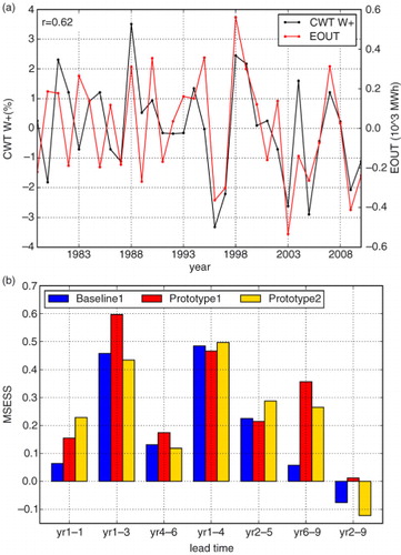
We therefore hypothesise that decadal forecast skill for regional Eout is high, if the MPI-ESM on the global scale is able to forecast the frequency of CWT W+ well. Figure 7b shows the MSESSs for annual CWT W+ frequencies for seven different lead times. Skill scores are positive for all lead times except yr2-9 in all three MPI-ESM ensemble generations. The skill scores for CWT W+ frequencies are similar to MSESSs for Eout (see Fig. 4b) and RPSSs for wind speed, with highest skill scores for short lead times and a decrease with increasing time since initialisation. As for wind energy, the highest positive skill score is found for yr1-3 for prototype1 (added value of initialisation of 60 %), while the highest value for yr2-5 is detected for prototype2. As a consequence, the decadal forecast skill for wind energy potentials can to some extend be attributed to an adequate forecast of the frequencies of strong westerly flow over Central Europe. Therefore, a potential source of forecast skill for regional wind energy potentials over Central Europe could be identified.

5. Summary and discussion

The decadal forecast skill for regional wind speed and wind energy potentials over Central Europe was investigated for three ensemble generations of the MiKlip decadal prediction system. The MPI-ESM ensembles have the same atmosphere initialisation but differ in their ocean initialisation. The performance of the global MPI-ESM and the regionalised hindcast ensembles was tested in terms of decadal predictability using different skill metrics (MSESS, RPSS and reliability). The main results of this study can be summarised as follows:

• All three ensemble generations show forecast skill for annual wind speeds and Eout over Central Europe. This skill is mostly limited to short lead times, with highest values for yr1-3, and is best for North-Western Germany and Benelux.

• In seasonal terms, forecast skill is best for autumn and worst for summer. The predictive skill for seasonal Eout is typically lower than for annual Eout.

• The differences between the three MiKlip ensemble generations are generally small. However, prototype1 slightly outperforms the other two generations for yr1-3.

• A dominant westerly weather type with a strong zonal flow (CWT W +) is identified as a potential source for the forecast skill of Eout over Central Europe. MSESSs for CWT W+ are similar to MSESSs for Eout for almost all lead times.

• The added value of downscaling for mean winds is identified in terms of both RPSSs and reliability but depends on the lead time and the hindcast generation.

The added value of downscaling was quantified in terms of mean wind speeds rather than wind energy output. This choice is motivated by the fact that only 6-hourly wind speeds are available for MPI-ESM, which does not enable an adequate computation of Eout (which requires hourly data).

The results of the presented forecast skill assessment depend strongly on the choice of the verification dataset. We have chosen a DD simulation of reanalysis data, since no gridded observations for wind and wind energy are available for Central Europe. Thereby, we assume that the high-resolution wind speeds simulated with DD are a good proxy for observed gridded wind speeds. Nevertheless, skill scores may change if gridded observations are used as a verification dataset.

The present results indicate that the decadal forecast skill for wind energy originates mainly from the initialisation, since high positive skill scores are mostly limited to the first years after initialisation. For longer lead times, this skill disappears. These findings are in line with Haas et al. (2015), who evaluated the decadal predictability of regional peak winds in the MiKlip ensemble baseline1 and also found highest skill scores for short lead times. The enhanced skill scores for higher percentiles are also consistent with results by Haas et al. (2015), who showed, for example, that the enhanced storminess over Central Europe in the early nineties (leading to enhanced peak winds at the surface) could be identified in the baseline1 hindcasts. Such skill is not found for lower percentiles (Haas et al., 2015; their figure 7).

We could not find a systematic improvement from the baseline1 ensemble to the prototype versions, thus giving evidence that there is generally no superior initialisation strategy in terms of anomaly- or full-field-initialisation for wind energy applications. This assessment agrees with Kruschke et al. (2015), who found no significant differences between the MiKlip generations for winter storm frequencies over the North Atlantic and Europe.

In this study, we have used the characteristics of one exemplary wind turbine. The consideration of power curves from other wind turbines would result in different Eout values. However, since these differences would be systematic for both the initialised hindcasts and the uninitialised historical runs, we assume that the results presented here are similar for other wind turbines and that the choice of turbine has only a small impact on our conclusions with respect to the decadal predictability (see also Reyers et al., 2016).

The detected decadal forecast skill for regional wind energy output exhibited a strong dependence on the representation of westerly CWTs (the dominant weather types for strong wind situations) in the MPI-ESM. If the occurrence of westerly CWTs, especially those with high pressure gradients, is forecasted well by the global hindcasts, predictive skill is found for both regional wind speeds and regional Eout.

For future work, the coupling of this large-scale weather type with low-frequency components like teleconnection patterns could be investigated. This may help to understand the mechanisms behind the decadal predictability for wind energy potentials. Another issue, which could be addressed, is the large uncertainties in the decadal predictability in the MPI-ESM, particularly in terms of the non-systematic skill dependency on lead times and seasons. Further investigations on the influence of the ensemble size and of the different initialisation strategies on the decadal predictability are also necessary. In this study, we considered only 10 of the 15 available members of the two prototype ensembles in order to compare the skill scores with the baseline1 ensemble (which only has 10 ensemble members). Future work could consider all 15 realisations by using the ‘fair’ variant of the RPSS (e.g. Ferro, 2014), which takes into account ensembles with a different number of members. Further, wind power generation statistics taking the wind farm distribution and installed power into account (e.g. Cannon et al., 2015; Drew et al., 2015) should be analysed.

The present results are encouraging regarding the establishment of a decadal prediction system for Central Europe. They clearly show that there is a potential for forecasts of wind energy potentials up to several years ahead. In addition, the used SDD approach proved to be adequate for an application to large datasets and could easily be applied to operational decadal prediction systems. The regionalisation preserves and sometimes increases the forecast skill of the global runs and improves the ensemble spread in some cases. This opens a wide range of options for end-user application.

6. Acknowledgements

This research was supported by the German Federal Ministry of Education and Research (BMBF) under the project ‘Probabilistic Decadal Forecasts for Central and Western Europe’ (MiKlip-PRODEF, contract 01LP1120A), which is part of the MiKlip consortium (‘Mittelfristige Klimaprognosen’, http://www.fona-miklip.de). We thank the ECMWF for the ERA-Interim reanalysis dataset and the Max-Planck-Institute (Hamburg, Germany) for providing the GCM data (MPI-ESM). We thank the German Climate Computer Centre (DKRZ, Hamburg) for computer and storage resources and the Climate Limited-area Modelling Community (CLM Community; http://www.cosmo-model.org) for providing the COSMO-CLM model. We thank the members of MiKlip Module C (Regionalisation) for discussions, and Simona Höpp for help with data processing. We are grateful for the comments of the two anonymous reviewers, which helped to improve the manuscript.

Notes

To access the supplementary material to this article, please see Supplementary files under ‘Article Tools’.

References

- Balmaseda M. A. , Mogensen K. , Weaver A. T . Evaluation of the ECMWF ocean reanalysis system ORAS4. Q. J. Roy. Meteorol. Soc. 2013; 139: 1132–1161. http://dx.doi.org/10.1002/qj.2063 .
- Barstad I. , Sorteberg A. , dos-Santos Mesquita M . Present and future offshore wind power potential in Northern Europe based on downscaled global climate runs with adjusted SST and sea ice cover. Renewable Energy. 2012; 44: 398–405.
- Cannon D. J. , Brayshaw D. J. , Methven J. , Coker P. J. , Lenaghan D . Using reanalysis data to quantify extreme wind power generation statistics: a 33 year case study in Great Britain. Renewable Energy. 2015; 75: 767–778. DOI: http://dx.doi.org/10.1016/j.renene.2014.10.024 .
- Dee D. P. , Uppala S. M. , Simmons A. J. , Berrisford P. , Poli P. , co-authors . The ERA-Interim reanalysis: configuration and performance of the data assimilation system. Q. J. Roy. Meteorol. Soc. 2011; 137: 553–597. http://dx.doi.org/10.1002/qj.828 .
- Doblas-Reyes F. J. , Andreu-Burillo I. , Chikamoto Y. , Garcia-Serrano J. , Guemas V. , co-authors . Initialized near-term regional climate change prediction. Nat. Commun. 2013; 4: 1715. http://dx.doi.org/10.1038/ncomms2704 .
- Drew D. R. , Cannon D. J. , Brayshaw D. J. , Barlow J. F. , Coker P. J . The impact of future offshore wind farms on wind power generation in Great Britain. Resour. Policy. 2015; 4: 155–171. DOI: http://dx.doi.org/10.3390/resources4010155 .
- Eade R. , Smith D. , Scaife A. , Wallace E. , Dunstone N. , co-authors . Do seasonal-to-decadal climate predictions underestimate the predictability of the real world?. Geophys. Res. Lett. 2014; 41: 5620–5628. DOI: http://dx.doi.org/10.1002/2014GL061146 .
- Ferro C. A. T . Comparing probabilistic forecasting systems with the brier score. Weather Forecast. 2007; 22: 1076–1088. DOI: http://dx.doi.org/10.1175/WAF1034.1 .
- Ferro C. A. T . Fair scores for ensemble forecasts. Q. J. Roy. Meteorol. Soc. 2014; 140: 1917–1923. http://dx.doi.org/10.1002/qj.2270 .
- Fuentes U. , Heimann D . An improved statistical-dynamical downscaling scheme and its application to the Alpine precipitation climatology. Theor. Appl. Climatol. 2000; 65: 119–135. DOI: http://dx.doi.org/10.1007/s007040070038 .
- General Electric. 2.5 MW wind turbine series GEA17007B. 2010. Online at: http://site.ge-energy.com/prod_serv/products/wind_turbines/en/downloads/GEA17007A-Wind25Brochure.pdf .
- Giorgetta M. A. , Jungclaus J. , Reick C. H. , Legutke S. , Bader J. , co-authors . Climate and carbon cycle changes from 1850 to 2100 in MPI-ESM simulations for the coupled model intercomparison project phase 5. J. Adv. Model. Earth Syst. 2013; 5: 572–597. DOI: http://dx.doi.org/10.1002/jame.20038 .
- Giorgi F. , Jones C. , Asrar G. R . Addressing climate information needs at the regional level: the CORDEX framework. Bull. World Meteorol. Organ. 2006; 58: 175–183.
- Goddard L. , Kumar A. , Solomon A. , Smith D. , Boer G. , co-authors . A verification framework for interannual-to-decadal prediction experiments. Clim. Dyn. 2013; 40: 245–272. DOI: http://dx.doi.org/10.1007/s00382-012-1481-2 .
- Haas R. , Pinto J. G . A combined statistical and dynamical approach for downscaling large-scale footprints of European windstorms. Geophys. Res. Lett. 2012; 39: L23804. DOI: http://dx.doi.org/10.1029/2012GL054014 .
- Haas R. , Reyers M. , Pinto J. G . Decadal predictability of regional-scale peak winds over Europe using the Earth System Model of the Max-Planck-Institute for Meteorology. Meteorol. Z. 2015. http://dx.doi.org/10.1127/metz/2015/0583 (in press).
- Hueging H. , Born K. , Haas R. , Jacob D. , Pinto J. G . Regional changes in wind energy potential over Europe using regional climate model ensemble projections. J. Appl. Meteorol. Climatol. 2013; 52: 903–917.
- Ilyina T. , Six K. D. , Segschneider J. , Maier-Reimer E. , Li H. , Núnez-Riboni I . Global ocean biogeochemistry model HAMOCC: model architecture and performance as component of the MPI-Earth system model in different CMIP5 experimental realizations. J. Adv. Model. Earth Syst. 2013; 5: 287–315. http://dx.doi.org/10.1029/2012MS000178 .
- International CLIVAR Project Office (ICPO). Data and Bias Correction for Decadal Climate Predictions. 2011. Online at: http://www.wrcp-climate.org/decadal/references/DCPP_Bias_Correction.pdf, compiled by CMIP-WGCM-WGSIP Decadal Climate Prediction Panel.
- IPCC. Field C. B. , Barros V. , Stocker T. F. , Qin D. , Dokken D. J. , Ebi K. L. , Mastrandrea M. D. , Mach K. J. , Plattner G.-K. , Allen S. K. , Tignor M. , Midgley P. M . Managing the risks of extreme events and disasters to advance climate change adaptation. A Special Report of Working Groups I and II of the Intergovernmental Panel on Climate Change.
- Jones P. D. , Hulme M. , Briffa K. R . A comparison of lamb circulation types with an objective classification scheme. Int. J. Climatol. 1993; 13: 655–663.
- Jungclaus J. H. , Fischer N. , Haak H. , Lohmann K. , Marotzke J. , co-authors . Characteristics of the ocean simulations in the Max Planck Institute Ocean Model (MPIOM) the ocean component of the MPI-Earth system model. J. Adv. Model. Earth Syst. 2013; 5: 422–446. http://dx.doi.org/10.1002/jame.20023 .
- Kharin V. V. , Boer G. J. , Merryfield W. J. , Scinocca J. F. , Lee W. S . Statistical adjustment of decadal predictions in a changing climate. Geophys. Res. Lett. 2012; 39: L19705. http://dx.doi.org/10.1029/2012GL052647 .
- Köhl A . Evaluation of the GECCO2 ocean synthesis: transports of volume, heat and freshwater in the Atlantic. Q. J. Roy. Meteor. Soc. 2015; 141: 166–181. http://dx.doi.org/10.1002/qj.2347 .
- Kruschke T. , Rust H. W. , Kadow C. , Leckebusch G. C. , Ulbrich U . Evaluating decadal predictions of northern hemispheric cyclone frequencies. Tellus A. 2014; 66: 22830. DOI: http://dx.doi.org/10.3402/tellusa.v66.22830 .
- Kruschke T. , Rust H. W. , Kadow C. , Müller W. A. , Pohlmann H. , co-authors . Probabilistic evaluation of decadal predictions of Northern Hemisphere winter storms. Meteorol. Z. 2015. DOI: http://dx.doi.org/10.1127/metz/2015/0641 .
- Marotzke J. , Müller W. A. , Vamborg F. S. E. , Becker B. , Cubasch U. , co-authors . MiKlip – a national research project on decadal climate prediction. Bull. Am. Meteorol. Soc. Submitted
- Meehl G. A. , Goddard L. , Boer G. , Burgman R. , Branstator G. , co-authors . Decadal climate prediction: an update from the trenches. Bull. Am. Meteorol. Soc. 2014; 95: 243–267. http://dx.doi.org/10.1175/BAMS-D-12-00241.1 .
- Meehl G. A. , Goddard L. , Murphy J. , Stouffer R. J. , Boer G. , co-authors . Decadal Prediction – Can it be skilful?. Bull. Amer. Meteor. Soc. 2009; 90: 1467–1485. DOI: http://dx.doi.org/10.1175/2009BAMS2778.1 .
- Mieruch S. , Feldmann H. , Schädler G. , Lenz C.-J. , Kothe S. , co-authors . The regional MiKlip decadal forecast ensemble for Europe: the added value of downscaling. Geosci. Model. Dev. 2014; 7: 2983–2999. http://dx.doi.org/10.5194/gmd-7-2983-2014 .
- Moccia J. , Wilkes J. , Pineda I. , Corbetta G . Wind energy scenarios for 2020. European Wind Energy Association Report, EWEA, 3p. 2014. Online at: http://www.ewea.org/fileadmin/files/library/publications/reports/EWEA-Wind-energy-scenarios-2020.pdf .
- Müller W. A. , Baehr J. , Haak H. , Jungclaus J. H. , Kröger J. , co-authors . Forecast skill of multi-year seasonal means in the decadal prediction system of the Max Planck Institute for Meteorology. Geophys. Res. Lett. 2012; 39: L22707. DOI: http://dx.doi.org/10.1029/2012GL053326 .
- Müller W. A. , Pohlmann H. , Sienz F. , Smith D . Decadal climate predictions for the period 1901–2010 with a coupled climate model. Geophys. Res. Lett. 2014; 41: 2100–2107. http://dx.doi.org/10.1002/2014GL059259 .
- Najac J. , Lac C. , Terray L . Impact of climate change on surface winds in France using a statistical-dynamical downscaling method with mesoscale modelling. Int. J. Climatol. 2011; 31: 415–430.
- Pineda I. , Azau S. , Moccia J. , Wilkes J . Wind in power – 2013 European statistics. European Wind Energy Association Report, EWEA, 3p. 2014. Online at: http://www.ewea.org/fileadmin/files/library/publications/statistics/EWEA_Annual_Statistics_2013.pdf (accessed 12 February 2015).
- Pinto J. G. , Neuhaus C. P. , Leckebusch G. C. , Reyers M. , Kerschgens M . Estimation of wind storm impacts over Western Germany under future climate conditions using a statistical-dynamical downscaling approach. Tellus A. 2010; 62: 188–201. http://dx.doi.org/10.1111/j.1600-0870.2009.00424.x .
- Pohlmann H. , Müller W. A. , Kulkarni K. , Kameswarrao M. , Matei D. , co-authors . Improved forecast skill in the tropics in the new MiKlip decadal climate predictions. Geophys. Res. Lett. 2013; 40: 5798–5802. http://dx.doi.org/10.1002/2013GL058051 .
- Pryor S. C. , Barthelmie R. J . Climate change impacts on wind energy: a review. Renew. Sustain. Energy Rev. 2010; 14: 430–437. http://dx.doi.org/10.1016/j.rser.2009.07.028 .
- Pryor S. C. , Barthelmie R. J. , Claussen N. E. , Drews M. , MacKellar N. , co-authors . Analyses of possible changes in intense and extreme wind speeds over Northern Europe under climate change scenarios. Clim. Dyn. 2012; 38: 189–208. http://dx.doi.org/10.1007/s00382-010-0955-3 .
- Pryor S. C. , Schoof J. T. , Barthelmie R. J . Climate change impacts on wind speeds and wind energy density in Northern Europe: empirical downscaling of multiple AOGCMs. Clim. Res. 2005; 29: 183–198.
- Raddatz T. J. , Reick C. H. , Knorr W. , Kattge J. , Roeckner E. , co-authors . Will the tropical land biosphere dominate the climate-carbon cycle feedback during the twenty-first century?. Clim. Dyn. 2007; 29: 565–574.
- Reyers M. , Moemken J. , Pinto J. G . Future changes of wind energy potentials over Europe in a large CMIP5 multi-model ensemble. Int. J. Climatol. 2016; 36: 783–796. DOI: http://dx.doi.org/10.1002/joc.4382 .
- Reyers M. , Pinto J. G. , Moemken J . Statistical-dynamical downscaling for wind energy potentials: evaluation and applications to decadal hindcasts and climate change projections. Int. J. Climatol. 2015; 35: 229–244. DOI: http://dx.doi.org/10.1002/joc.3075 .
- Rockel B. , Will A. , Hense A . Special issue: regional climate modelling with COSMO-CLM (CCLM). Meteorol. Z. 2008; 17: 347–348.
- Sillmann J. , Croci-Maspoli M . Present and future atmospheric blocking and its impact on European mean and extreme climate. Geophys. Res. Lett. 2009; 36: L10702. DOI: http://dx.doi.org/10.1029/2009GL038259 .
- Smith D. M. , Cusack S. , Colman A. , Folland C. , Harris G. , co-authors . Improved surface temperature prediction for the coming decade from a global circulation model. Science. 2007; 317: 796–799.
- Solomon A. , Goddard L. , Kumar A. , Carton J. , Deser C. , co-authors . Distinguishing the roles of natural and anthropogenically forced decadal climate variability implications for predictions. Bull. Am. Meteorol. Soc. 2011; 92: 141–156. http://dx.doi.org/10.1175/2010BAMS2962.1 .
- Solomon S. , Qin D. , Manning M. , Chen Z. , Marquis M , co-authors . Climate Change 2007: The Physical Science Basis.
- Stevens B. , Giorgetta M. , Esch M. , Mauritsen T. , Crueger T. , co-authors . Atmospheric component of the MPI-M Earth System Model: ECHAM6. J. Adv. Model. Earth Syst. 2013; 5: 146–172.
- Taylor K. E. , Stouffer R. J. , Meehl G. A . An overview of CMIP5 and the experiment design. Bull. Am. Meteorol. Soc. 2012; 93: 485–498. http://dx.doi.org/10.1175/BAMS-D-11-00094.1 .
- Tobin I. , Vautard R. , Balog I. , Bréon F. M. , Jerez S. , co-authors . Assessing climate change impacts on European wind energy from ENSEMBLES high-resolution climate projections. Clim. Change. 2014; 128: 99–112. DOI: http://dx.doi.org/10.1007/s10584-014-1291-0 .
- Uppala S. M. , Kallberg P. W. , Simmons A. J. , Andrae U. , da Costa Bechthold V. , co-authors . The ERA-40 re-analysis. Q. J. Roy. Meteor. Soc. 2005; 131: 2961–3012. http://dx.doi.org/10.1256/qj.04.176 .
- Valcke S. , Claubel A. , Declat D. , Terray L . OASIS Ocean Atmosphere Seas Ice Soil User's Guide. DOI: http://dx.doi.org/10.1007/s00382-012-1313-4 .
- Van Oldenborgh G. J., Doblas-Reyes F. J., Wouters B., Hazeleger W. Decadal prediction skill in a multi-model ensemble. Clim. Dyn. 2012; 38: 1263–1280. DOI: http://dx.doi.org/10.1007/s00382-012-1313-4.
- Weigel A. P. , Liniger M. A. , Appenzeller C . Seasonal ensemble forecast: are recalibrated single models better than multi-models?. Mon. Wea. Rev. 2009; 137: 1460–1479.
- Wilks D. S . Statistical Methods in the Atmospheric Sciences. 2011; Academic Press, Oxford; Waltham, MA. 3rd ed.