Rainfall downscaling of weekly ensemble forecasts using self-organising maps

Abstract

This study presents an application of self-organising maps (SOMs) to downscaling medium-range ensemble forecasts and probabilistic prediction of local precipitation in Japan. SOM was applied to analyse and connect the relationship between atmospheric patterns over Japan and local high-resolution precipitation data. Multiple SOM was simultaneously employed on four variables derived from the JRA-55 reanalysis over the area of study (south-western Japan), and a two-dimensional lattice of weather patterns (WPs) was obtained. Weekly ensemble forecasts can be downscaled to local precipitation using the obtained multiple SOM. The downscaled precipitation is derived by the five SOM lattices based on the WPs of the global model ensemble forecasts for a particular day in 2009–2011. Because this method effectively handles the stochastic uncertainties from the large number of ensemble members, a probabilistic local precipitation is easily and quickly obtained from the ensemble forecasts. This downscaling of ensemble forecasts provides results better than those from a 20-km global spectral model (i.e. capturing the relatively detailed precipitation distribution over the region). To capture the effect of the detailed pattern differences in each SOM node, a statistical model is additionally concreted for each SOM node. The predictability skill of the ensemble forecasts is significantly improved under the neural network-statistics hybrid-downscaling technique, which then brings a much better skill score than the traditional method. It is expected that the results of this study will provide better guidance to the user community and contribute to the future development of dam-management models.

• self-organizing maps
• weekly ensemble forecasts
• downscaling

1. Introduction

Improvement of long-term weather forecasts is one of the primary goals of weather services. One common means to improve weather prediction is the development and improvement of numerical forecast models, and much effort has been assigned through the initial conditions, resolution and physical parameterisations of subgrid scale processes. In recent decades, ensemble forecast techniques have also been developed as a tool for probability forecast. Medium-range (3–10 d) ensemble forecasts are one such endeavour and are crucial for reducing the impact of extreme events such as floods and heat waves. They also provide more time for decision-making and preparation than short-range (1–2 d) forecasts. In particular, probabilistic medium-range forecasts based on ensemble forecasts increase the capability of early weather warnings such as floods (Cloke and Pappenberger, 2009) and add value for emergency management (as demonstrated in the Hydrological Ensemble Prediction Experiment, Schaake et al., 2007) by providing more confidence than deterministic forecasts currently used in many weather prediction centres by the given associated uncertainties.

Potential end-users of medium-range forecasts in different sectors (e.g. hydrology and renewable energy) sometimes need high-resolution forecasted surface data, such as surface wind speed, air temperature and rainfall, to drive their models. For instance, hydrological models calculate river discharge processes involving slow reservoirs and rapid evolution of precipitation fields. Therefore, the medium-range hydrological prediction is highly dependent on the quality of input atmospheric variables. However, in general, the spatial resolution of general circulation models used in forecasts is still low (20–200 km) for the prediction of surface information which is of relevance to end-users. Downscaling methods are often used to produce output at the smaller spatial scales required by the majority of end users. Much research has focussed on the methods and availability of dynamical and empirical (statistical- or neural network-based methods) downscaling over the last 20 yr (Wilby and Wigley, 1997; Maraun et al., 2010). In empirical downscaling, local climate is assumed to be a function of the large-scale climatic state and physical features of the local environment. Typically, in the case of empirical precipitation downscaling, a perfect prognosis (PP) approach in which an empirical/statistical relationship is established between local observations and simultaneously observed large-scale predictors is often taken and then applied to simulated predictors derived from a global model. The goal of PP is to derive an empirical link between a set of large-scale ‘predictor’ variables (e.g. temperature, humidity, wind or geopotential height) and a local-scale ‘predictand’ (e.g. precipitation). In contrast, dynamical downscaling uses higher resolution regional models, which are nested into global models over a limited area, in order to represent physical processes at a high resolution. As the dynamical approach is constrained by computational expense (and the availability of regional models), the empirical method is a popular alternative because of its relative ease of use and general performance comparable to the output of regional models.

Due to the very large amount of data provided in medium-range ensemble forecasts, efficient analysis and downscaling tools such as PP are required to extract useful information. The approach by using data mining techniques is an advanced type of statistical/empirical methods for both analysis and downscaling tools (Han and Kamber, 2000). The self-organising map (SOM), developed by Kohonen (1982), is one of the most common data mining techniques that is capable of projecting high-dimensional non-linear features onto a visually understandable two-dimensional map. Attempting to overcome the problem of downscaling a large number of ensemble forecasts, some recent studies (e.g. Gutiérrez et al., 2005; Chattopadhyay et al., 2008; Borah et al., 2013) have proposed the use of a SOM-based analogue technique for downscaling of forecasts to precipitation. The original analogue method (Lorenz, 1969) is based on the assumption that if the current (targeted) condition is similar to those of past condition, the local weather can be similar to that of the past. This original technique has traditionally been used in studies of downscaling (Zorita and von Storch, 1999; Timbal and McAvaney, 2001; Obled et al., 2002; Garcia-Morales and Dubus, 2007). Gutiérrez et al. (2005) and Hewitson and Crane (2006) developed SOM-based downscaling methods for multimodel forecasts and future projections. Chattopadhyay et al. (2008) and Borah et al. (2013) also attempted to predict intraseasonal oscillations using an SOM-based technique, which gave reasonable forecasts four pentads in advance. SOM have an advantage of making a non-parametric relationship of predictor and predictands. Therefore, this PP approach requires few statistical assumptions to formulate the downscaling model.

Statistical/empirical algorithms such as PP improve raw numerical forecasts by implicitly calibrating the predictable from the unpredictable. The goal of this study is to evaluate the ability of the SOM-based precipitation downscaling technique at forecasting probabilities of local precipitation for medium-range lead times, which uses atmospheric forecasts from the Japan Meteorological Agency (JMA) Ensemble Prediction System (EPS). In this study, we apply SOM for analysing a space of daily weather patterns (WPs) over Japan and attempt the PP approach for ensemble forecasts to predict local weekly precipitation. This empirical downscaling of ensemble forecasts results in substantial improvements in prediction skill for local precipitation that implies that the application of fast PP techniques (like used in this study) will increase decision-making capabilities in the user communities, such as the electric power industry.

This study is organised as follows. Section 2 represents a description of the data set and method used in this study. Section 3 shows the results of the downscaling technique and examines the change in predictability skill. Finally, Section 4 provides a summary of the conclusions of this study.

2. Data and downscaling method

2.1. Data

We use atmospheric data for the period 1958–2008 obtained from the Japanese 55-yr Reanalysis (JRA-55; Ebita et al., 2011). The horizontal resolution of the atmospheric fields is 1.25°. Since the present study focusses on daily-mean precipitation, we use historical daily-mean high-resolution (0.05°×0.05°) precipitation data ‘APHRO_JP’ over Japan from the product ‘Asian Precipitation–Highly-Resolved Observational Data Integration Towards Evaluation of the Water Resources’ (APHRODITE) project. This rainfall data are mainly based on rain gauge observations and then have an accurate representation of both mean and extreme values. The details of the data are documented in Kamiguchi et al. (2010).

The scope of this study is to evaluate precipitation predictions that use atmospheric forecasts from the EPS and to validate the ability of the technique at probabilistic forecast of local precipitation for medium-range (1 week in this study) lead times. We use atmospheric ensemble forecasts, specifically a TL319 (approximately 60-km resolution) 60-level version of JMA-EPS. The EPS constructs 51 ensemble members each day (12 UTC) by perturbing initial conditions. In this study, EPS data from 2009 to 2011 is used. For comparison, we also use deterministic (i.e. no ensemble) forecasts, a TL959 (approximately 20-km resolution) 60-level version of JMA Global Spectral Model (GSM) for the same period with one of the highest horizontal resolutions of operational global models.

The boreal early summer (from 1 June to 31 July; JJ) and late summer (from 1 August to 30 September; AS) are targeted in this study because these periods are the most hazardous weather seasons in Japan. During June to July, heavy rainfall events occur frequently in Japan because of the intrusion of warm moist air into a stationary Baiu front. Several extreme events in Japan correspond with the intensified Baiu activity, which induces flooding with serious damage to life and property. After the rainy season (i.e. during the late summer), summer heat waves occur in many locations. However, several typhoons that often bring heavy rainfall events also strike Japan during this season. Most of the typhoons that strike Japan arrive in September, generally come ashore in southern Japan.

2.2. SOM technique

As an artificial neural network, we use the SOM technique (Kohonen, 1982) in this study. Various advantages of the technique, including it being a powerful visualisation approach, have been described (e.g. Iseri et al., 2009). Because SOM can obtain a spatially organised set of patterns from temporally varying input data, it has been used in meteorological studies such as climate characterisation (Reusch et al., 2007; Johnson and Feldstein, 2010), identification of model errors and model evaluation (Radić and Clarke, 2011; Kolczynski and Hacker, 2014), and analysis of extreme events (Cavazos, 1999; Nishiyama et al., 2007; Ohba et al., 2015). These previous studies successfully separate visually clear-cut WPs from complex non-linear relationships.

We apply SOM to cluster a space of daily WPs over Japan during the period 1958–2008 (the periods corresponding to the available JMA weekly EPS data are eliminated) and link it to local precipitation. The method of WP classification by SOM is same as that in Ohba et al. (2015). As the input vector of SOM, we concatenated multiple normalised atmospheric variables into one vector for each day. The SOM technique projects these input vectors onto regularly arranged two-dimensional arrays. Each of the arrays is referred as a node, which has one reference vector (the dimensions is same as the input vector). The summary of the SOM projection process is as follows: (1) Each input vector is compared with all reference vectors and the best-matching node is identified by using the Euclidean distance. (2) The best-matching node and neighbourhood reference vectors are updated by the input vector. (3) The processes (1) and (2) are repeated for each input vector for a large number of cycles while reducing the neighbourhood region. Eventually, each reference vector is approximately the mean of assigned data vectors to the SOM pattern and the input data is classified into a two-dimensional plane based on similarities of the patterns. The reference vectors that are located relatively nearby (distant) on the SOM mean relatively similar (dissimilar) pattern. Instead of conventional SOM, we use torus-SOM (Ito et al., 2000), which has no difference of neighbourhood sets and no edge in the map. We make five SOM maps consisting of 16×16, 18×18, 20×20, 22×22 and 24×24 neurons (i.e. 256, 324, 400, 484 and 576 WPs). The result of the 20×20 map is used as a representative of the maps, and it is the only result shown.

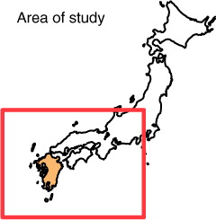
We simultaneously apply SOM to four atmospheric variables obtained from JRA-55 around western Japan (127.5°E–137.5°E, 30°N–36.25°N; Fig. 1) for the period 1958–2008. Four variables are selected as input for SOM: anomalous 850-hPa equivalent potential temperature (θ_e), 850-hPa zonal wind, 850-hPa meridional wind and 300-hPa geopotential height (GH). θ_e is a thermodynamic parameter involving both humidity and temperature and the low-level advection to western Japan from the tropics sometimes results in heavy rainfall on the region. The positions of the upper-level jet stream are also important for the intensity of rainfall that variations can be seen in 300-hPa GH. The anomalies are identified by removing the 5-d running averaged climatology and standardised (normalised) by dividing them with the standard deviation to get each variable on a similar range.

Fig. 1 Area of study in south-west Japan (red solid box) used to define the atmospheric patterns. The orange shading represents the Kyushu region used in Section 3b.

The result of WP classification by SOM can be characterised by the distribution of rainfalls. For each SOM node, we also take a subset of the related daily precipitation (in all of the days in the node) to estimate the mean and probabilistic local precipitation. We develop a precipitation probability density function (PDF) of gamma distribution for each SOM node, according to the histogram for each precipitation grid. In precipitation analysis, there is a need for finding suitable models that correctly capture the data behaviour. The rainfall amounts are usually estimated based on the assumption that they follow a certain PDF. Several such distributions have been used such as the one-parameter exponential distribution, two parameter gamma, Weibull distributions and three-parameter skewed normal and mixed exponential distributions. The gamma distribution is often assumed to be suitable for distributions of daily precipitation and has been proven to be effective for the analysis of precipitation data. As for the sampling of the daily precipitation data to make the PDF, we use the node-weighted sampling. The samplings are obtained from nine nodes (the targeted node and eight neighbouring nodes), while the eight neighbouring nodes are assigned lower (half) weights compared with the centre-targeted node.

2.3. Rainfall downscaling method based on SOM

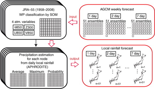
The SOM technique is used in this study to increase the spatial resolution of the EPS by creating the relationship between atmospheric fields and daily local precipitation. Each SOM node defines the daily precipitation corresponding to each WP. Based on this link between the SOM-derived WPs (represented by reference vectors) and related local precipitation, we can obtain a forecast PDF of daily precipitation prediction from atmospheric variables of the EPS. This can be regarded as an alternative to conventional analog (Lorenz, 1969; Wilby and Wigley, 1997; Zorita and von Storch, 1999) or analog ensemble (Delle Monache et al., 2013) techniques presented in the previous studies. We extract the same variables from the EPS for the same region that we used to train the SOM. We then standardise the EPS data using the same values as we used for JRA-55. Afterwards, each WP of the ensemble forecasts is assigned to its best-match node, based on its distance from the reference vectors. For each season (JJ and AS), 51 forecast patterns are available daily. The composited PDF of the local forecast is finally obtained from the PDF assigning the local precipitation to each node and each of the grids. Since the locations of the precipitation data (APHRO_JP) define the locations of the downscaling targets, the rainfall downscaling is conducted at the resolution of the observation, that is, the 0.05° grid in this case. This downscaling technique is applied to south-western Japan for early and late summer, respectively. A schematic diagram of the algorithm of the downscaling technique is shown in Fig. 2 and summarised below.

1. First, five different SOMs (16×16, 18×18, 20×20, 22×22 and 24×24) are applied for the atmospheric variables (top-left panel).

2. For each node of (1), local precipitation patterns and its gamma PDF are estimated (picked up from observational data; bottom-left panel).

3. Using the SOM (1), pick up the node best matching the 51 ensemble forecasts in the EPS (top-right panel) from the five SOM maps, respectively.

4. By compositing the five individual results obtained in (3), 51 precipitation ensemble forecasts and then PDF are derived (bottom-right panel).

5. The ensemble mean of the rainfall PDF for each station (grid) is obtained from (4). The best estimate of the local (regional/watershed area mean) rainfall intensity is also obtained by the subempirical model (see later) for each ensemble member.

Fig. 2 Schematic diagram of the SOM-based downscaling method. The five different SOM classifications of the WP are based on the normalised anomalies of four atmospheric variables for June–July and August–September during 1958–2009 (top left). Based on the SOM lattices, the precipitation PDF patterns are estimated for each node (bottom left). By using the SOM lattice, the downscaled precipitation is obtained (bottom right) from the 51 daily members of the EPS produced for 7 d (top right).

Eckert et al. (1996) also applied SOMs to summarise forecast members of EPS and introduced the entropy to characterise the ensemble spread in a relatively similar methodology. Although the present study uses a similar methodology, we provide local precipitation downscaling of operative medium-range forecasts, as was conducted for seasonal forecasting in Gutiérrez et al. (2005).

The SOM downscaling scheme is sensitive to selection of the parameters, for example, SOM dimension size and atmospheric variables. Sensitivity to the choice of input was tested by using other variables (such as 500-hPa GH, 850-hPa GH and 500-hPa wind). Standard deviation of the precipitation for each SOM node is used as the evaluation metrics of the WP–precipitation relationship. It could be conceivable that the lower internode mean of the standard deviation can be regarded as more robust WP–precipitation relationship. The obtained best combination is used in this study. For example, previous studies (e.g. Ninomiya and Shibagaki, 2007) for the Baiu front suggest that the advection of an equivalent potential temperature that consists of a moisture flux by the low-level jet is important to the active Baiu rainband around Japan. Yoshikane et al. (2001) also reported that the rainband is quite sensitive to not only the low-level current but also the positions of the upper-level jet stream, which is significantly influenced by 200/300-hPa GH. The results of previous studies are consistent with the selection of the variables in this study.

Although SOM patterns are obtained from four coupled variables, the forecast outputs may not always be coupled with each other. To capture the detailed response of the precipitation and obtain the best estimate, we also incorporate a substatistical model for each SOM node. This statistical model is constructed for each SOM node after the SOM classification that is a complementary tool to the SOM downscaling. In this study, we use simple multiregression model for the four atmospheric variables. This model obtains the deviations of precipitation values from each SOM node mean. In addition to the PDF estimation, this internode model estimates more accurate regional (watershed area) mean rainfall which could also provide useful information. Several studies have attempted to identify the local rainfall intensity responsible for the WP evolution by statistical methods (Zorita and von Storch, 1999). The obtained best estimates by the additional statistical models could reduce forecast error. As first, to reduce the number of degrees of freedom, empirical orthogonal function (EOF) analysis is applied to the respective four variables, and the resultant principal components of the seven leading EOFs are used as the predictors to the predictands (the measured local climate variables, i.e. regional mean precipitation). The statistical model used in this study is developed using standard multilinear regression analysis, and regression coefficients are obtained for each of the SOM nodes. The seven leading EOFs are respectively obtained from the four variables, and 28 principal components (PCs) are used. The temporal evolutions of the forecasted PCs are defined here by the projection onto the 28 EOFs.

3. Rainfall downscaling of weekly ensemble forecasts

3.1. Effect of the downscaling method

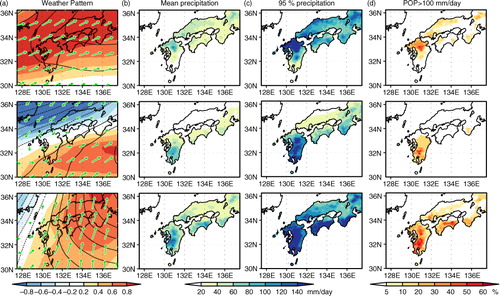
Rainfall can have various atmospheric origins and can be non-linearly related to various meteorological factors. Classification of the (synoptic-scale) weather background condition could be useful for understanding and improving rainfall forecast (Garavaglia et al., 2010, 2011; Brigode et al., 2013). First, in this section, we show the result of the SOM analysis conducted for JRA-55. Figure 3a represents three examples of anomalous WPs (mean atmospheric condition corresponding to the reference vector) derived from the 20×20 SOM analysis for JJ. Areas of high pressure at 300 hPa are shown by solid contours. Red (blue)–shaded regions indicate relatively high (low) θ_e at the 850-hPa level, and green vectors represent the 850-hPa wind. These variables are respectively normalised to equalise the weight of each variable, and day-by-day WPs are classified for the nodes. We also show the corresponding mean (Fig. 3b), 95th percentile of local precipitation (Fig. 3c) and probability of precipitation exceeding 100 mm/day (Fig. 3d) in relation to each WP. The three patterns are selected as representative of the WPs that can result in relatively strong precipitation corresponding with the dominant heavy rainfall patterns in Japan as discussed in Ohba et al. (2015). From this figure, we can see the impact of WP on the local rainfall. Corresponding with the intrusion of high θ_e at the low level of atmosphere, the local precipitation responses to the WPs are significantly different. For example, for the WP at the top of Fig. 3a, the western Japan is covered by low-level westerly winds with intrusion of warm moist air (high θ_e). The intrusion and convergence of moist air over the land is very effective at producing the deep convection over the northern part of western Japan that produces relatively strong precipitation (top of Fig. 3b). However, the northward intrusion of moist air results in precipitation over the southern part of the region (bottom of Fig. 3b). The rainfall intensity of the precipitation pattern is relatively amplified in the mountainous region, but it is reduced in the rain shadow region, namely showing geographically varying differences in the nature of precipitation. This result implies that different WPs can result in differences of the rainfall distribution by implicitly including the effect of topography on the rainfall.

Fig. 3 Three examples of anomalous WPs derived from the 20×20 SOM non-linear classification. (a) Node-averaged (composited) daily-mean 850-hPa θ_e (K: red–blue shading), 300-hPa GH (m: black contour) and 850-hPa wind (m/s: green vectors) anomalies. The WP-related (b) mean precipitation, (c) 95th percentile precipitation and (d) 100 mm/day rainfall rate (%; probability of precipitation) for each node.

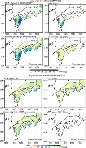
Figure 4 shows the precipitation for observation (upper left), the 20-km GSM (upper right), ensemble-mean downscaled precipitation (lower left) and raw precipitation (lower right) of EPS (60-km GSM) in the 1-d forecast for 6 August 2011 (Fig. 4a) as well as the mean of August–September 2011 (Fig. 4b). The downscaled precipitation here is obtained from the node mean in the SOM. As expected, because of the relatively low spatial resolution of the EPS, the precipitation response in the EPS raw precipitation cannot capture either the spatial distribution or the intensity of local precipitation (lower right in Fig. 4a and b). However, by using the SOM-based empirical downscaling, the predicted precipitation captures relatively well the overall features (such as orographic precipitation) found in the observed precipitation. The seasonal mean (AS) precipitation is also significantly improved (lower left in Fig. 4b). It is conceivable that the weekly ensemble via the downscaling provides comparable or better results (detailed precipitation distribution) with those of the 20-km high-resolution GSM.

Fig. 4 (a) Daily mean precipitation (mm/day) on 6 August 2011 for observed, 20 km GSM (no ensemble), SOM downscaling (ensemble mean) and 60-km GSM (ensemble mean). (b) is same as (a) except for August–September.

A heavy rainstorm caused by a stationary front (Baiu front) struck the northern Kyushu region from 19 to 26 July 2009. The Kyushu region is the region shaded orange in Fig. 1. An extraordinarily strong rainstorm was recorded in the region, and it resulted in widespread flash flooding, landslides and debris flow disasters that claimed the lives of about 30 people. Rainfall totals during this 1 week exceeded 600 mm in the centre of northern Kyushu. Figure 5a shows the footprint of 51 weekly ensembles on the SOM lattice predicted from 19 July 2009. The solid box in Fig. 5 represents the actual state (closest WP, i.e., best matching node of the reanalysis). It is worth mentioning here that the top (right) edge of the 20×20 SOM lattice is connected to the bottom (left) edge because we used the torus-type SOM. The frequency occurrence of each SOM pattern results from mapping the 51 ensembles to the SOM. If the ensemble forecasts are ‘perfect’, there would be a very dark square with solid black box for the pattern matched by the reanalysis data indicating that all forecast ensembles matched the observations. The spread of boxes indicates the range of skill of the ensemble members and this varies according to forecast days. The WP frequencies of the ensemble forecasts extend gradually on the SOM while maintaining the aggregation to some extent. In this case, it is conceivable that the medium-range ensemble forecast captures relatively well the atmospheric condition of the actual state (except for the day 4 forecast). This analysis provides an effective way to visually grasp the broadening of ensembles.

Fig. 5 (a) SOM frequency (best matched) of the 51 ensemble members on the 20×20 SOM lattice for forecast days 1–7. Solid black box represents the actual state. (b) Daily mean precipitation obtained from the downscaling for forecast days 1–7. The spread of the ensemble for GSM raw is presented by the green-shaded box (EPS raw). The node-mean downscaled precipitation (S-DS) and its ensemble mean are represented by black ‘×’ mark and horizontal bar, respectively. Composited PDFs of downscaled precipitation obtained from the SOM are represented by red error bar. Observational precipitation (actual state) is represented by the grey bar.

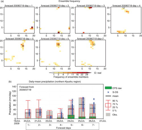
We also show the daily mean precipitation averaged over the northern Kyushu region for this case (Fig. 5b), as obtained from the precipitation downscaling of the ensemble forecasts. Green error bars represent the ensemble spread (minimum to maximum) of the raw precipitation output obtained from the EPS, whereas the red error bars with box plots represent the ensemble-mean PDF obtained from the downscaling. The best estimate of precipitation intensity obtained from the submodel is represented by blue ‘x’ mark. By using the downscaling of precipitation, the precipitation of EPS is significantly improved. In the first and second day of the period, the mean of downscaled precipitation almost agrees with the observational result. The PDF also covers the observed precipitation. Although the precipitation for the 4-d forecast is significantly overestimated (Fig. 5a, forecast day = 4), it could be a result of the failure to capture the actual WP by GSM prediction or the predicted pattern cannot be captured by the SOM classified WPs (because of the problem of SOM node number/variables or the WP is not experienced in the historical record). However, the solid boxes are overlapped with coloured squares in the other forecast days suggesting that the signal of an atmosphere, which can potentially bring heavy precipitation, is included in the spread of the ensembles. As for the second half of the period, the empirical downscaling captures relatively well the high risk of heavy rainfall to some extent, but this not the case in GCM direct rainfall. Because the best estimates of each ensemble forecast member extend gradually, the PDF approaches the climatological PDF and the day-to-day difference is reduced.

3.2. Predictability skill of the downscaling

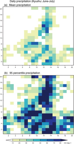
In this subsection, we evaluate the predictability of local precipitation obtained from the downscaling of the ensemble forecasts. As for the example of the predictability of precipitation, the regionally averaged rainfall over the Kyushu region (Fig. 1, orange region) is evaluated for 2009–2011. The Kyushu Islands, at the western edge of Japan, frequently experience heavy rainfall corresponding with synoptic situations such as enhanced Baiu front activity and landfall of typhoons during the early and late summer, respectively. The daily precipitation averaged over the Kyushu region on the 20×20 SOM lattice is shown in Fig. 6a. Relatively wet WPs (i.e. exceeding 30 mm/day rainfall) are mainly in the centre, top-right and bottom of the SOM, whereas the top-left and top-right corner are relatively dry. The 95th percentile daily mean precipitation value reaches 80 mm in many nodes and shows strong contrast among the nodes on the lattice. The strong contrast of rainfall among the nodes implies that the WP classification can potentially provide fruitful information for estimate of the regional rainfall.

Fig. 6 Daily precipitation (mm/day) averaged over the Kyushu region for (a) node-mean and (b) 95th percentile on the 20×20 SOM lattice during June–July.

We now show the results of the downscaling using the JRA-55 as a predictor to simply illustrate the performance of the method. Figure 7 represents the results of the downscaling for western Japan during June and September 2011. The black horizontal bars with blue error bars in this figure show the regional mean daily precipitation obtained by the substatistical model described above, and the red error bars with box plots show the PDF obtained from the SOM nodes. The empirical model captures relatively well the day-by-day variation of observed precipitation, and the magnitude of the precipitation is included in the 95th percentile in the best-match node.

Fig. 7 Forecasted daily mean precipitation obtained from the downscaling by using JRA-55 as predictor during (a) June and (b) September 2011. Black horizontal bar represents the estimated precipitation by the substatistical model and the error bar 2-sigma. Composited PDFs of downscaled precipitation obtained from the best-match SOM nodes are represented by red error bar (5th, 25th, 75th and 95th percentiles). Observational precipitation (actual state) is represented by the grey bar.

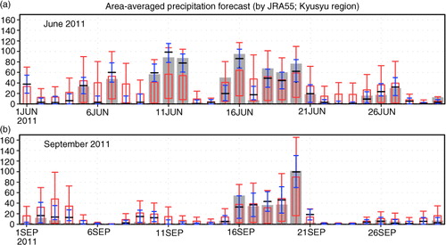
Figures 8 and 9 show the results of the downscaling of EPS for western Japan during June and September 2011, respectively. The red error bars with box plots in this figure show the ensemble-mean PDF of the daily precipitation. Furthermore, the downscaled precipitation obtained from the submodel and its ensemble means are represented by the blue dots (each error bar is muted for visibility) and black horizontal lines. The spread of the ensemble members (i.e. blue dots) provides an indication of the likely accuracy of the ensemble mean forecast. The predicted precipitation for each forecast day (1, 3, 5, 7 day lead times) is shown separately. Because of the simplicity of this estimation method, the PDF results in a relatively wide range of structures. In this region, the ensemble mean of the model predicts relatively well (i.e. most of the observed precipitation is included in the 95th percentile) the precipitation during both June and September (especially for forecast day 1), but the predicted amounts are smaller than the observed amounts (depicted by shaded bar) on most of the wet days. The prediction skill is decreased gradually and the extent of the ensemble spread is increased with respect to the forecast length, which may be a result of a convergence of the forecast PDF towards the climatological PDF. Although the forecast uncertainty varies substantially from day to day around forecast day 3, at forecast day 7 it is almost similar from day to day.

Fig. 8 Same as Fig. 7 except for forecast day 1, 3, 5 and 7 of EPS during June 2011. The downscaled precipitation by the substatistical model and its ensemble mean are represented by blue dots and black horizontal bars, respectively.

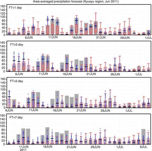
Fig. 9 Same as Fig. 8 except for September 2011.

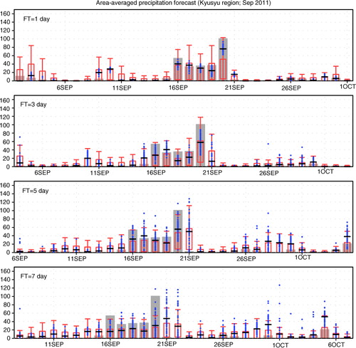
In late September 2011, a persistent and unusually powerful tropical cyclone, Typhoon Roke, affected Japan (especially the main island of Honshu) and resulted in the deaths of 16 people through hazards such as widespread flooding triggered by the heavy rains. The Kyushu region experienced relatively strong precipitation from 16 to 20 September. The downscaled precipitation captured relatively well the potential increase in rainfall around the period through the different lead times. The day-by-day contrast seen in forecast day 1 decreases gradually, and the intensity extends around day 1 before and after.

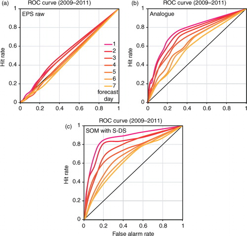
We can assess this downscaling framework in probabilistic form by calculating the probability that a given threshold value is exceeded. One of the well-used verification methods for probabilistic forecasts is the relative operating characteristic (ROC). ROC evaluates the ability of forecasts to aid decision-making by measuring the signal intensity in the forecast. ROC curves are plotted from the basis of contingency tables for the number of forecast occurrences, forecast non-occurrences, observed occurrences and observed non-occurrences (Jolliffe and Stephenson, 2003). To check the skill of the downscaled forecasts, we show ROC curves obtained from the raw EPS data, nearest-neighbours analogue method (Fig. 10b) and SOM downscaling of this study (Fig. 10c) applied to the EPS (each 1- to 7-d forecast) for the whole periods (JJ and AS in 2009–2011). The nearest-neighbours analogue method was conducted as a conventional method for comparison of the results. Its local precipitation is obtained from the observed precipitation showing the highest similarity in the atmospheric variables among the reanalysis data. In the ROC curves, the area under the curve indicates the skill of the forecast system. A perfect forecast system yields a full area (1), whereas a curve lying along the diagonal (0.5) means essentially worthless forecast. In this study, contingency tables were constructed by rainfall thresholds set at 0, 1, 2, 4, 8, 16, 32, 64, 128 and 256 mm/day. As expected, the precipitation values in the raw EPS data have basically no predictability skill (Fig. 10a). However, the predictability skill of the precipitation is improved significantly in both PP methods (Fig. 10b and c). The area under the ROC curve decreases with increasing forecast lead time for both PP approaches, while it remains above the no-skill threshold (0.5) at all of the forecast lead times. The SOM-based method has a relatively good skill score (i.e. larger area under the curve) compared with the conventional method, despite the decrease in the computational cost. This improvement may be attributed to the effect of WP clustering and the additional use of the substatistical model.

Fig. 10 ROC curves for forecast days 1–7 for the precipitation of (a) GSM raw, (b) analogue method and (c) SOM downscaling for the periods of June–July and August–September in 2009–2011.

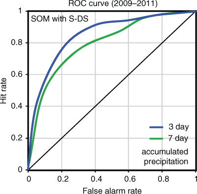
The forecast skill of accumulated precipitation is useful as an early warning for possible flooding/drought and management of dams. We also show the upcoming 3-d and 7-d accumulated precipitations predicted in JJ 2010 as an example (Fig. 11). The accumulated precipitation is calculated by summing the daily observed and forecast rainfall. The observed accumulated precipitation is forecast relatively well by the downscaling of EPS, but some dates have significantly over/under estimated precipitation, such as around 26 June. The ROC curve of both accumulated precipitations for the period 2009–2011 (Fig. 12) shows relatively good prediction skill, which is nearly equivalent to that of 1- or 2-d predictions (Fig. 10c).

Fig. 11 Same as Fig. 8 except for forecast 3-d and 7-d accumulated precipitation in June–July 2010.

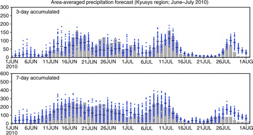
Fig. 12 ROC curves for the forecast 3-d and 7-d accumulated precipitation of SOM downscaling for the periods June–July and August–September in 2009–2011.

4. Discussion and summary

In this study, we show the application of SOM for rainfall downscaling of weekly (medium-range) forecasts conducted by the JMA EPS to support the availability of hydrological forecasts. Precipitation in Japan exhibits strong variability during summer. The complex relationships between synoptic-scale WPs and local observational data were linked to get the local weather information around Japan by using the SOM algorithm. We represented the applications of the SOMs not only for analysing ensemble forecasts but also for the downscaling of precipitation based on ideas used in previous studies (Cavazos, 1999; Gutiérrez et al., 2005; Hewitson and Crane, 2006). The skill of the probabilistic local forecasts of the rainfall downscaling was evaluated for the Kyushu region (western edge of Japan). From the result of downscaling, we showed that precipitation associated with WPs can be predicted some days in advance and therefore that the predictability skill of precipitation is improved significantly by the PP approach. The SOM-based downscaling can be an effective technique when a very large number of ensemble forecasts are used. The obtained high-resolution long-term probabilistic forecasts can be fruitful as an information source for end-user's decision-making such as operation of a flood control dam.

The multimodel ensemble surpasses the single ensemble for both a deterministic forecast and a probability forecast, as was already shown in many studies by using multimodel ensemble forecasts such as the TIGGE (Park et al., 2008) and ENSEMBLES (Hewitt, 2005). It is well known that each model has individual systematic errors, thus multimodel ensemble can provide more realistic estimates than individual forecasts through the cancellation of errors (Matsueda and Tanaka, 2008; Johnson and Swinbank, 2009). The methodology presented in this study offers an (computationally) inexpensive method that can be employed quickly with various ensemble forecast outputs while using the single model EPS. We will attempt the use of such multimodel data in a future study. Questions also may remain about the relative availability of this empirical downscaling compared with dynamical downscaling. While they are not capable of incorporating various feedback processes at the local scale, our method is particularly favourable from the aspect of computational cost and quickly gives a first-order estimate of local impacts that is physically consistent with the simulated WPs. We demonstrate the potential of empirical techniques to combine a very huge number of ensemble forecast data with minimal computational cost.

5. Acknowledgements

We thank Drs. J. Tsutsui, H. Hirakuchi and M. Matsueda for their constructive discussions.

References

- Borah N. , Sahai A. K. , Chattopadhyay R. , Joseph S. , Abhilash S. , co-authors . Self-organizing map-based ensemble forecast system for extended range prediction of active/break cycles of Indian summer monsoon. J. Geophy. Res. Atmos. 2013; 118: 1–13.
- Brigode P. , Mićović Z. , Bernardara P. , Paquet E. , Garavaglia F. , co-authors . Linking ENSO and heavy rainfall events over Coastal British Columbia through a weather pattern classification. Hydrol. Earth Syst. Sci. 2013; 17: 1455–1473.
- Cavazos T . Large-scale circulation anomalies conducive to extreme precipitation events and deviation of daily rainfall in northeastern Mexico and southeastern Texas. J. Clim. 1999; 12: 1506–1523.
- Chattopadhyay R. , Sahai A. K. , Goswami B. N . Objective identification of nonlinear convectively coupled phases of monsoon intraseasonal oscillation: implications for prediction. J. Atmos. Sci. 2008; 65: 1549–1569.
- Cloke H. L. , Pappenberger F . Ensemble flood forecasting: a review. J. Hydrol. 2009; 375: 613–626.
- Delle Monache L. , Eckel T. , Rife D. , Nagarajan B . Probabilistic weather prediction with an analog ensemble. Mon. Wea. Rev. 2013; 141: 3498–3516.
- Ebita A. , Kobayashi S. , Ota Y. , Moriya M. , Kumabe R. , co-authors . The Japanese 55-year Reanalysis ‘JRA-55’: an interim report. SOLA. 2011; 7: 149–152.
- Eckert P. , Cattani A. , Ambühl J . Classification of ensemble forecasts by means of an artificial neural network. Meteorol. Appl. 1996; 3: 169–178.
- Garavaglia F. , Gailhard J. , Paquet E. , Lang M. , Garcon R. , co-authors . Introducing a rainfall compound distribution model based on weather patterns sub-sampling. Hydrol. Earth Syst. Sci. 2010; 14: 951–964.
- Garavaglia F. , Lang M. , Paquet E. , Gailhard J. , Garcon R , co-authors . Reliability and robustness of rainfall compound distribution model based on weather pattern sub-sampling. Hydrol. Earth Syst. Sci. 2011; 15: 519–532.
- Garcia-Morales M. B. , Dubus L . Forecasting precipitation for hydroelectric power management: how to exploit GCM's seasonal ensemble forecasts. Int. J. Climatol. 2007; 27: 1691–1705.
- Gutiérrez J. M. , Cofiño A. S. , Cano R. , Sordo C . Analysis and downscaling multi-model seasonal forecasts in Peru using self-organizing maps. Tellus A. 2005; 57: 435–447.
- Han J. , Kamber M . Data mining: Concepts and Techniques. 2000; Morgan-Kaufman, San Francisco.
- Hewitson B. C. , Crane R. G . Consensus between GCM climate change projections with empirical downscaling: precipitation downscaling over South Africa. Int. J. Climatol. 2006; 26: 1315–1337.
- Hewitt C. D . The ENSEMBLES Project: providing ensemble-based predictions of climate changes and their impacts. EGGS Newslett. 2005; 13: 22–25.
- Iseri Y. , Matsuura T. , Iizuka S. , Nishiyama K. , Jinno K . Comparison of pattern extraction capability between self-organizing maps and principal component analysis. Memoirs of Faculty Engineering . Kyushu Univ. 2009; 69: 37–47.
- Ito M. , Miyoshi T. , Masuyama H . The characteristics of the torus self organizing map. Proc. Fuzzy. Syst. Symp. 2000; 16: 373–374.
- Johnson N. C. , Feldstein S. B . The continuum of North Pacific sea level pressure patterns: intraseasonal, interannual, and interdecadal variability. J. Clim. 2010; 23: 851–867.
- Johnson C. , Swinbank R . Medium-range multimodel ensemble combination and calibration. Q. J. Roy. Meteorol. Soc. 2009; 135: 777–794.
- Jolliffe I. T. , Stephenson D. B . Forecast Verification: A Practitioner's Guide in Atmospheric Science. 2003; Wiley, Chichester, 240 pp.
- Kamiguchi K. , Arakawa O. , Kitoh A. , Yatagai A. , Hamada A. , co-authors . Development of APHROJP, the first Japanese high-resolution daily precipitation product for more than 100 years. Hydrol. Res. Lett. 2010; 4: 60–64.
- Kohonen T . Self-organized formation of topologically correct feature maps. Biol. Cybern. 1982; 43: 59–69.
- Kolczynski W. C. , Hacker J. P . The potential for self-organizing maps to identify model error structures. Mon. Wea. Rev. 2014; 142: 1688–1696.
- Lorenz E. N . Atmospheric predictability as revealed by naturally occurring analogs. J. Atmos. Sci. 1969; 26: 639–646.
- Matsueda M. , Tanaka H. L . Can MCGE outperform the ECMWF ensemble?. SOLA. 2008; 4: 77–80.
- Maraun D., Wetterhall F., Ireson A. M., Chandler R. E., Kendon E. J., co-authors. Precipitation downscaling under climate change. Recent developments to bridge the gap between dynamical models and the end user. Rev. Geophys. 2010; 48: 3003. DOI: http://dx.doi.org/10.1029/2009RG000314.
- Ninomiya K., Shibagaki Y. Multi-scale features of the Meiyu-Baiu front and associated precipitation systems. J. Meteor. Soc. Jpn. 2007; 85B: 103–122. DOI: http://dx.doi.org/10.2151/jmsj.85B.103.
- Nishiyama K. , Endo S. , Jinno K. , Uvo C. B. , Olsson J. , co-authors . Identification of typical synoptic patterns causing heavy rainfall in the rainy season in Japan by a self-organizing map. Atmos. Res. 2007; 83: 185–200.
- Obled C. , Bontron G. , Garcon R . Quantitative precipitation forecasts: a statistical adaptation of model outputs through an analogues sorting approach. Atmos. Res. 2002; 63: 448–463.
- Ohba M. , Nohara D. , Yoshida Y. , Kadokura S. , Toyoda Y . Anomalous weather patterns in relation to heavy precipitation events in Japan during the Baiu season. J. Hydrometeorology. 2015; 16: 688–701.
- Park Y. Y. , Buizza R. , Leutbecher M . TIGGE: preliminary results on comparing and combining ensembles. Q. J. R. Meteorol. Soc. 2008; 134: 2029–2050.
- Radić V. , Clarke G . Evaluation of IPCC models’ performance in simulating late-twentieth-century climatologies and weather patterns over North America. J. Clim. 2011; 24: 5257–5274.
- Reusch D. B., Alley R. B., Hewitson B. C. North Atlantic climate variability from a self-organizing map perspective. J. Geophys. Res. 2007; 112: 02104. DOI: http://dx.doi.org/10.1029/2006JD007460.
- Schaake J. C. , Hamill T. M. , Buizza R. , Clark M . HEPEX, the hydrological ensemble prediction experiment. Bull. Am. Meteorol. Soc. 2007; 88: 1541–1547.
- Timbal B. , McAvaney B. J . An analogue-based method to downscale surface air temperature: application for Australia. Clim. Dyn. 2001; 17: 947–963.
- Wilby R. L. , Wigley T. M. L . Downscaling general circulation model output: a review of methods and limitations. Prog. Phys. Geog. 1997; 21: 530–548.
- Yoshikane T., Kimura F., Emori S. Numerical study on the Baiu front genesis by heating contrast between land and ocean. J. Meteor. Soc. Jpn. 2001; 79: 671–686. DOI: http://dx.doi.org/10.2151/jmsj.79.671.
- Zorita E. , von Storch H . The analog method as a simple statistical downscaling technique: comparison with more complicated methods. J. Clim. 1999; 12: 2474–2489.