A comparison of the equivalent weights particle filter and the local ensemble transform Kalman filter in application to the barotropic vorticity equation

Abstract

Data assimilation methods that work in high-dimensional systems are crucial to many areas of the geosciences: meteorology, oceanography, climate science and so on. The equivalent weights particle filter (EWPF) has been designed for, and recently shown to scale to, problems that are of use to these communities. This article performs a systematic comparison of the EWPF with the established and widely used local ensemble transform Kalman filter (LETKF). Both methods are applied to the barotropic vorticity equation for different networks of observations. In all cases, it was found that the LETKF produced lower root mean–squared errors than the EWPF. The performance of the EWPF is shown to depend strongly on the form of nudging used, and a nudging term based on the local ensemble transform Kalman smoother is shown to improve the performance of the filter. This indicates that the EWPF must be considered as a truly two-stage filter and not only by its final step which avoids weight collapse.

• equivalent weights particle filter
• non-linear data assimilation
• EMPIRE
• LETKF
• nudging
• LETKS relaxation

1. Introduction

1.1. Data assimilation and Bayes’ theorem

When making a prediction based on a dynamical model of a system, it is necessary to initialise that model. This could be done simply by guessing the initial conditions of such a model or, as is more common, confronting the model with observations of the system.

Such observations necessarily have errors associated with them and also tend to be incomplete. That is, they are not direct observations of every component of the model. The mathematical formulation of how to rigorously incorporate such observations into the model is Bayes’ theorem (Bayes and Price, 1763; Jazwinski, 1970):

In this equation, x represents the model state and y the observations. Hence, the posterior probability density function (pdf) p(x ∣ y) is given as the product of the likelihood p(y ∣ x) with the prior p(x) and normalised by the pdf of the observations p(y). Different approximations of Bayes’ theorem lead to different methods of data assimilation. For instance, if one reduces the problem to finding a local mode of the posterior pdf, this becomes an inverse problem which can be solved by variational techniques: the famous 3DVar and 4DVar methods (see e.g. Le Dimet and Talagrand 1986; Dashti et al. 2013).

1.2. Particle filters

A particle filter is a Monte Carlo approach to computing the posterior via Bayes’ theorem [see e.g. Doucet et al. (2001) or van Leeuwen (2009)] in the context of a dynamically evolving system.

Without loss of generality, suppose that we have the prior pdf, p(x ^k ), at timestep k written as a finite sum of delta functions (formally distributions),where δ(x) is the standard Dirac delta function. The set of state vectors is known as the ensemble, and each state vector is referred to interchangeably as a particle or ensemble member. Note that in this notation the prior is arbitrary: it may depend on any data that have previously been assimilated and may have been evolved from a known probability density at a previous time. This information will be encoded into the weights . As p(x ^k ) is a pdf, , which implies , and p(x ^k ) ≥ 0 implies .

We have a model for the dynamics of the state which is Markovian:3 where f is a deterministic model and β ^k is a stochastic model error term. To evolve the prior in time, we note that from the definition of conditional probability,4

Now following Gordon et al. (1993), p(x ^k+1 ∣ x ^k ) is a Markov model defined by the statistics of β ^k that are assumed known:5

As β ^k is independent of the state x ^k , p(β ^k ∣ x ^k )=p(β ^k ) and we have6

Substituting eq. (2) and eq. (6) into eq. (4), we obtain7

Integrating over x ^k , this reduces to8

Now for each ensemble member i, we make a single draw from p(β ^k ), (i.e. ) so that9 that is, .

Now, we suppose some observations of the system, y, at timestep n. What we desire is a representation of the posterior pdf at timestep n, p(x ⁿ ∣ y). To do this, we can use the weighted delta function representation of the prior in combination with Bayes’ theorem (1):10

Hence, the weights in the posterior pdf are the normalised product of the prior weights and the pointwise evaluation of the likelihood. For any subsequent timesteps, the posterior is used as the prior in a recursive manner.

Filter degeneracy, or weight collapse, is the scenario in which for some j ∈ 1,…,N _e . Hence, . In this case, the first-order moment of the posterior pdf, , will be simply . All higher order moments will be computed to be approximately 0.

Snyder et al. (2008) showed that, in the case of using a naive particle filter such as the sequential importance resampling (SIR) filter (Gordon et al., 1993), to avoid filter degeneracy the number of ensemble members must be chosen such that where N _τ is a measure of the dimension of the system. Ades and van Leeuwen (2013) showed that this dimension of the system is actually the number of independent observations.

Simply increasing the number of ensemble members is, for most geophysical applications, infeasible. N _e will be determined by the size of the supercomputer available. For operational numerical weather prediction (NWP) methods, N _e may typically be around 50. For instance, simply for forecasting, the Canadian NWP ensemble forecast uses N _e =20, the European Centre for Medium-Range Weather Forecasts has N _e =51 and the UK Met Office has N _e =46.

Therefore, it is clear that for a particle filter to represent the posterior pdf successfully, the case that for some j ∈ 1, …, N _e should be avoided. The equivalent weights particle filter (EWPF) (van Leeuwen, 2010) that we shall discuss in Section 2 is designed specifically so that for all i ∈ 1, …, N _e . It does this in a two-stage process. Firstly, the particles are nudged towards the observations. Secondly, an ‘equivalent weights step’ is made to avoid filter degeneracy.

1.3. Ensemble Kalman filters

The Ensemble Kalman filter (EnKF) is a method of data assimilation that attempts to solve Bayes’ theorem when assuming that the posterior pdf is Gaussian [see e.g. (Evensen 1994; Burgers et al. 1998; Evensen 2007)]. In that case, the posterior can be characterised by its first two moments: mean and covariance. The prior pdf, or more precisely the covariance of the prior, is represented by an ensemble of model states. Instead of propagating the full covariance matrix of the prior by a numerical model [as in the Kalman filter (Kalman, 1960)], only the ensemble members are propagated by the model.

If the dimension of the model state, N _x , is much greater than the number of ensemble members used, N _e , then the EnKF is much more computationally efficient than the Kalman filter.

Defining X _k to be the scaled matrix of perturbations of each ensemble member from the ensemble mean at time k, then the update equation of the EnKF can be written as11 Here, refers to the forecast of the ensemble member at time k and the resulting analysis ensemble member at time k which has been influenced by the observations. H is the observation operator that maps the model state into observation space, and R is the observation error covariance matrix.

There are many different flavours of ensemble Kalman filter, each of which is a different way to numerically compute the update equation. For a discussion on the different kinds see, for example, Tippett et al. (2003) and Lei et al. (2010). In this article, we shall consider implementing the EnKF by means of the local ensemble transform Kalman filter (LETKF) and shall discuss this in detail in Section 3.

1.4. Motivation for this investigation

We have seen that if we are trying to use a particle filter to recover the posterior pdf via a numerical implementation of Bayes’ theorem, then it makes sense to ensure that the weights of each particle are approximately equal. Or at least, it pays to ensure that each particle has non-negligible weight, specifically when higher order moments of the posterior pdf are required.

Until now, there has been no systematic comparison of the EWPF and an ensemble Kalman filter using a non-trivial model of fluid dynamics. This is a necessary study to see if anything is gained by not making the assumptions of Gaussianity that are made by the EnKF method. Previous investigations of the EWPF have focused on tuning the free parameters in the system to give appropriate rank histograms. In this study, we shall investigate the method's ability to appropriately constrain the system in idealised twin experiments.

To this end, the system we shall consider is the equations of fluid dynamics under the barotropic vorticity (BV) assumptions. This is perhaps the model most well studied for the EWPF. As a system of one prognostic variable on a two-dimensional grid, it is easily understood and affordable to experiment with. We also know the parameter regimes in which the EWPF will perform well.

The remainder of this article is organised as follows. In Section 2, we discuss the use of proposal densities within particle filters before introducing the EWPF. In Section 3, we discuss the LETKF. In Section 4, we discuss the BV model which we consider. In Section 5, we define the experimental setup which we use and performance measures. In Section 6, we show the numerical results that are discussed in detail in Section 7. Finally in Section 8, we finish with some conclusions and discuss the implications for full-scale NWP.

2. Particle filters using proposal densities

In this section, we briefly summarise the use of a proposal density within a particle filter, before going on to discuss the specific choices of these made in the EWPF.

2.1. Proposal densities

A key observation that has advanced the field of particle filters is the freedom to rewrite the transition density as12 which holds so long as the support of q(x ^k+1 ∣ x ^k ,y) is larger than that of p(x ^k+1 ∣ x ^k ). Now, we are also free to change the dynamics of the system such that13 as in the study by van Leeuwen (2010). As in Section 1.2, we assume that, without loss of generality, we have a delta function representation for the prior at timestep k given by eq. (2). Then, in a manner similar to the marginal particle filter (Klaas et al., 2005),14 15 16

We can write the transition density and proposal density in terms of β ^k :17

Now, similarly to before, drawing a single sample for each ensemble member, but now from the distribution q(β ^k ), gives That is,21 where22

To find the delta function representation of the posterior, it is the case of combining this derivation with Bayes’ theorem to arrive at the same equation as in eq. (10).

The use of proposal densities is the basis of particle filters such as the implicit particle filter (Chorin and Tu, 2009) and the EWPF, and more recently the implicit equal weights filter (Zhu et al., 2016). The goal is to choose the proposal density in such a way that the weights do not degenerate.

2.2. The equivalent weights particle filter

The EWPF is a fully non-linear data assimilation method that is non-degenerate by construction. For a comprehensive overview of the EWPF see van Leeuwen (2010) and Ades and van Leeuwen (2013).

A key feature of the EWPF is that it chooses the proposal density q(x ^k+1∣x ^k ,y) equal to p(β ^k ) but with new mean g(x ^k ,y). It proceeds in a two-stage process with one form of g(x ^k ,y) for the timesteps that have no observations and a different form of g(x ^k ,y) when there are observations to be assimilated.

For each model timestep k+1 before an observation time n, the model state of each ensemble member, , is updated via the equation23 where y ⁿ is the next observation in time, H is the observation operator that maps the model state onto observation space and A is a relaxation term. In this work, we consider24 where the matrices Q and R correspond to the model evolution error covariance and observation error covariance matrices, respectively. σ(k) is a function of time between observations; in this article, σ(k) increases linearly from 0 to a maximum (σ) at observation time. Equations (23) and (24) together make up what we will refer to as the nudging stage of the EWPF. This process is iterated until k+1=n−1.

In this work, we consider only unbiased Gaussian model error [i.e. ]. To obtain a formula for the un-normalised weights at timestep k+1, we can use this Gaussian form in eq. (22). Taking logarithms leads to a formula for the weights of the particles (van Leeuwen, 2010; Ades and van Leeuwen, 2015) as

The second stage of the equivalent weights filter involves updating each ensemble member at the observation time n using the term26 where α _i are scalars computed so as to make the weights of the particles equal. This is done for a given proportion (0<κ≤1) of the ensemble which can make the desired weight. The remaining ensemble members are resampled using stochastic universal sampling (Baker, 1987; van Leeuwen, 2010).

It is important to realise that the covariance of the prior ensemble is never explicitly computed in the EWPF but implicitly, via the EWPF approximation to Bayes’ theorem: increasing the spread in the prior will increase the spread in the posterior. Instead, the covariance of the error in the model evolution Q is crucial.

3. Local ensemble transform Kalman filter

The LETKF is an implementation of the ensemble Kalman filter which computes in observation space (Bishop et al., 2001; Wang et al., 2004; Hunt et al., 2007). As with all ensemble Kalman filters, the pdfs are assumed Gaussian. Formally, the LETKF update equation for ensemble member i at the observation timestep n can be written as27 where is the mean of the forecast ensemble at timestep n, is the ensemble of forecast perturbations and is the column of a weighting matrix corresponding to ensemble member i. Full details of this is given in Hunt et al. (2007). This can be extended through time (Posselt and Bishop, 2012) such that for k<n, we get the local ensemble transform Kalman smoother (LETKS) update equation28

As typically the number of ensemble members will be much fewer than the dimension of the model state, spurious correlations will occur within the ensemble. These spurious correlations lead to information from an observation inappropriately affecting the analysis at points far away from the observation. To counteract this, the LETKF effectively considers each point in the state vector separately and weights the observation error covariance by a factor depending on the distance of the observation from the point in the state vector.

For each point in the state vector, the inverse of the observation error covariance matrix, R ⁻¹ (also known as the precision matrix), is weighted by a function w so that

The weighting of the observation error covariance matrix R is given by the function29 where d is the distance between the point in the state vector and the observation and l is a predefined localisation length scale.

In the case of a diagonal R matrix, then

The weighting w(d) is a smoothly decaying function which cuts off when , that is, w(d)⁻²=e ⁻⁸≈0.0003. This means that the computations are speeded up by ignoring all the observations which have a precision less than 0.0003 of what they were originally.

Inflation is typically also required for the LETKF in large systems (Anderson and Anderson, 1999). That is, the ensemble perturbation matrices are multiplied by a factor of (1+ρ) in order to increase the spread in the ensemble that is too small because of undersampling, that is, X _f → (1+ρ) X _f in eq. (27).

4. Barotropic vorticity model

In this section, we consider the model which we investigate. We start with the Navier–Stokes equations and assume incompressible flow, no viscosity, no vertical flow and that flow is barotropic [i.e. ρ=ρ(p)]. We define vorticity q to be the curl of the velocity field. This results in the following partial differential equation in q [see e.g. Krishnamurti et al. (2006)], known as the BV model,

where u is the component of velocity in the x direction and v is the component of velocity in the y direction. The domain we consider is periodic in both x and y and so the computation of this can be made highly efficient by the use of a fast Fourier transform (FFT). In order to solve this equation, it is sufficient to treat vorticity q as the only prognostic variable. The curl operator can be inverted in order to derive the velocity field u from the vorticity. We use a 512×512 grid, making N _x =2¹⁸, a 262,144 dimensional problem. Timestepping is achieved by a leapfrog scheme with dt=0.04 (roughly equivalent to a 15-minute timestep of a 22-km resolution atmospheric model). The decorrelation timescale of this system is approximately 42 timesteps or 1.68 time units.

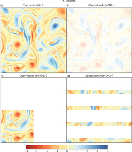
There are a number of good reasons for investigating this model. For example, it exhibits strong non-linear behaviour, develops cyclonic activity and generates fronts. All of which are typical of the highly chaotic regimes occurring in many meteorological examples. Turbulence in the model is prototypical: energy is transferred downscale due to the presence of non-linear advection (see Fig. 2a for a plot of a typical vorticity field from the model). Note that it was the BV model that was used for some of the earliest numerical weather predictions (Charney et al., 1950).

Note that this model has no balances that can be destroyed by data assimilation, something which should be considered in other studies of this kind. A further advantage for this first study is that we do not have to worry about bounded variables when applying the LETKF.

Also for this model we know the parameter regimes and model error covariance structure for which the EWPF performs well. Ades and van Leeuwen (2015) first applied the EWPF to the BV model, albeit at a lower resolution, and in this article, we employ similar parameters in the EWPF such as the nudging strength σ(k) and use the same model error covariance matrix Q. The Ades and van Leeuwen (2015) study concentrated on using rank histograms as the performance diagnostic of the EWPF, whereas in this article we consider performance in terms of root meansquared errors (RMSE).

5. Experimental setup

In this section, we discuss the two experiments we shall run. All of the experiments were carried out using the EMPIRE data assimilation codes (Browne and Wilson, 2015) on ARCHER, the UK national supercomputer.

5.1. Model error covariance matrix

For ensemble methods in the NWP setting, obtaining spread in the ensemble is a key feature in the performance of both the analysis and the forecast. In NWP applications, this is typically achieved by employing a stochastic physics approach (Baker et al., 2014) or using a stochastic kinetic energy backscattering (Tennant et al., 2011) to add randomness at a scale which allows the model to remain stable. For the EWPF (or indeed any particle filter that uses a proposal density), we must specify (possibly implicitly) the model error covariance matrix. Understanding and specifying the covariances of model error in a practical model is a challenge to which much more research must be dedicated.

The model error covariance matrix used in this article is the same as that used in Ades and van Leeuwen (2015). That is, Q is a second-order autoregressive matrix based on the distance between two grid points, scaled so that the model error has a reasonable magnitude in comparison with the deterministic model step.

5.2. Initial ensemble

The initial ensemble is created by perturbing around a reference state. Thus, for each ensemble member x _i and the true state x _t ,30

The background error covariance matrix B is chosen proportional to Q such that B=20² Q. The reference state x _r is a random state which is different for each experiment.

5.3. Truth run for twin experiments

The instance of the model that is considered the truth is propagated forward using a stochastic version of the model where

5.4. Observing networks

We shall show results from experiments with three different observing networks that make direct observations of vorticity. The first is regular observations throughout the domain as considered by Ades and van Leeuwen (2015), the second is a block of dense observations and the third is a set of strips that could be thought of as analogous to satellite tracks. The details of the observing networks are shown below and visualised in Fig. 1.

Fig. 1 Observing network diagrams.

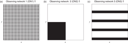
ON1: Every other point in the x and y directions observed

ON2: Only those points such that (x,y) ∈ [0,0.5]×[0,0.5] are observed

ON3: Only those points such that (x,y) ∈ [0,1]×([0,0.0675] ∪ [0.25,0.3175] ∪ [0.5,0.5675] ∪ [0.75,0.8175]) are observed

In each case, we have N _y =N _x /4=65 536. The observation errors are uncorrelated, with a homogeneous variance such that R=0.05² I. Observations occur every 50 model timesteps. These observations are quite accurate when you consider that the vorticity typically lies in the interval (−4, 4) (see Fig. 2a).

Fig. 2 Plots of vorticity for the true state and the resulting observations using the different networks at the 6th analysis time, for a particular random seed.

5.5. Comparison runs

For comparison and analysis purposes, we will run a number of different ensembles as well as the LETKF and the EWPF. We detail these subsequently.

5.5.1. Stochastic ensemble.

Each ensemble member is propagated forward using a stochastic version of the model. That is,

5.5.2. Simple nudging.

For each timestep, the nudging terms of the EWPF are used to propagate the model forward. That is, eqs. (13), (23) and (24) are used to update the model state. The weights of the particles are disregarded, and the ensemble is treated as if it was equally weighted.

5.5.3. Nudging with an LETKS relaxation.

The model is propagated forward in time stochastically until the timestep before the observations. During this stage, no relaxation term is used (i.e. g(x ^k ,y)=0). At the timestep before the observations, the relaxation term that is used comes from the LETKS. That is, term in eq. (23) is the increment that would be applied by the LETKS. At the observation timestep, the ensemble is propagated using the stochastic model. The weights of the particles are disregarded, and the ensemble is treated as if it was equally weighted.

This can be written in equation form, so that at each iteration k before the observation time n, the update for each ensemble member i is given by31 where g _i is the increment arising from the LETKS for ensemble member i.

5.5.4. The EWPF with an LETKS relaxation.

Similarly to nudging with the LETKS relaxation, the model is propagated forward in time stochastically until the timestep before the observations. At the timestep before the observations, the relaxation that is used comes from the LETKS. At the observation timestep, the equivalent weights step (26) of the EWPF is used. The weights are calculated using eq. (22) which in this case with Gaussian model error remains, given explicitly by eq. (25). We employ κ=0.75, 0.25 and 0.5 for observation networks 1, 2 and 3, respectively. This is discussed in Section 7.3.

5.6. Assimilation experiments

Observations occur every 50 timesteps for the first 500 model timesteps. After that, a forecast is made from each ensemble member for a further 500 timesteps.

For each observing network, we run five different experiments:

• The EWPF

• The LETKF

• Simple nudging

• Nudging with an LETKS relaxation

• The EWPF with an LETKS relaxation

Table and 2 list the parameter choices used for the different methods for the different observational networks. They were chosen by performing a parameter sweep across the various free parameters and selecting those that gave the lowest RMSEs (shown in Fig. A1).

Table 1. Parameter values used in the LETKF

Observation network	1	2	3
Localisation length scale, l	0.005	0.02	0.007
Inflation factor, ρ	0.01	0.01	0.01

Table 2. Parameter values used in the EWPF

Observation network	1	2	3
Keep proportion, κ	1.0	1.0	1.0
Nudging factor, σ	0.7	0.5	0.7

All of these experiments are repeated 11 times. In each of the 11 experiments, the initial reference state, x _r , is different, as is the random seed used. For reference, we also run a stochastically forced ensemble from each of the different reference states. As no data is assimilated here, these runs are independent of the observing network.

We choose to run 48 ensemble members for each method. This is for two reasons: there are 24 processors per node on ARCHER so this is computationally convenient, and 48 is of the order of the number of ensemble members that operational NWP centres are currently using.

6. Results

6.1. Root mean–squared errors

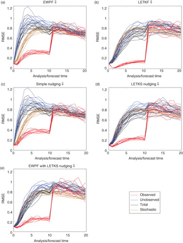
Figures 3 to 5 show RMSE for the different assimilation methods on the three separate observing networks. Formally, the RMSE we show is the square root of the spatial average of the square of the difference from the ensemble mean and the truth. Each line of the similar colour refers to a distinct experiment with a different stochastic forcing and initial reference state. Values are shown only for the initial ensemble, 10 analysis times (recall that each analysis time is separated by 50 model time steps) and 10 subsequent forecast times that are again separated by 50 model timesteps.

Fig. 3 Observing network 1, every other gridpoint. The total and unobserved RMSEs are almost exactly underneath the observed RMSE plots. This is due to the widespread information from the observations effectively constraining the whole system.

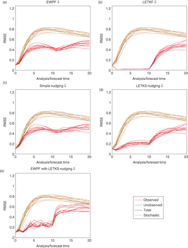
In brown, for reference, is plotted the RMSE from the stochastically forced ensemble; in black, the total RMSE; in blue, the unobserved variables; and in red, the observed variables.

The RMSE, as defined previously, is a measure of the similarity of the ensemble mean to the truth. If the posterior is a multimodal distribution, then the ensemble mean may be far from a realistic, or accurate, state. EnKF methods, by their Gaussian assumptions that they make, naturally assume a unimodal posterior. Particle filters on the contrary do not make such an assumption. In this article, we do not investigate the effect of using a different error measure.

Figure 3 is markedly different from Figs. 4 and 5 – in this case, the unobserved variables behave as if they are also observed. This is because each unobserved variable is either directly adjacent to two observed variables or diagonally adjacent to four observed variables. Contrast this with the observing networks 2 and 3 where an unobserved variable could be a maximum of 181 or 48 grid points, respectively, away from an observed variable.

Fig. 4 Observing network 2, block of dense observations.

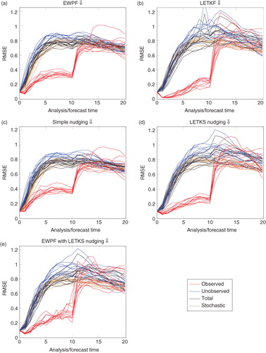
Fig. 5 Observing network 3, tracks of observations.

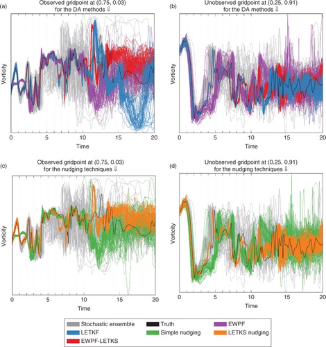
6.2. Trajectories of individual grid points

In Fig. 6, we show the evolution of the vorticity at a given grid point for a single experiment. Every model timestep is shown for each of the ensemble members for the different methods.

Fig. 6 Trajectories of two different points in the domain when using the different assimilation methods with observing network 3 for a single experiment.

7. Discussion

It is clear from the results presented that the EWPF with simple nudging, as implemented by Ades and van Leeuwen (2015), is not competitive with the LETKF in terms of RMSEs. This is similar to the results noted in Browne and van Leeuwen (2015) in that the EWPF gives RMSEs higher than the error in the observations.

In this section, we shall discuss different aspects of the results, in an attempt to give some intuition as to why they occur.

7.1. RMSEs from the EWPF are controlled by the nudging term

Consider the differences between RMSE plots for the simple nudging and the EWPF. They are qualitatively similar [Figs. 3–5, (a) vs. (c)]. Further, when we use a different type of nudging [Figs. 3–5, (d) vs. (e)], the results are again similar.

This is due to the two-stage nature of the EWPF. The first stage is a relaxation towards the observations (23), followed by a stage at observation time which ensures against filter degeneracy (26). In the second stage, we are not choosing the values of α _i to give a best estimate in some sense (e.g. compare with the best linear unbiased estimator) but instead they are chosen so that the weights remain equal. Hence, most of the movement of the particles towards the observations happens in the first, relaxation, stage.

This is shown strongly in Fig. 6; the simple nudging and the EWPF are qualitatively similar. Also in Fig. 6, it can be seen that the LETKS nudging and the EWPF–LETKS also follow similar trajectories. This shows that the equivalent weights step of the EWPF is not moving the particles very far in state space in order to ensure the weights remain equal.

7.2. Simple nudging is insufficient to get close to the observations

Figures 3c, 4c, and 5c show that, with simple nudging, the RMSEs are much larger than the observation error standard deviation. This is due to the choice of nudging equation used (24).

The goal of nudging is to bring the particles closer to the observations, or equivalently, to the area of high probability in the posterior distribution. In this section, we shall discuss the properties that this nudging term should have.

Let the nudging term be denoted as A(x,y) and written as a product of operatorswhere A _I is the innovation, A _w is the innovation weighting, A _m is the mapping from observation space to state space and A _s is the operator to spread the information from observation space throughout state space.

The innovation should have the form

where f takes the state at the current time and propagates it forward to the corresponding observation time. With this, the innovation is exactly the discrepancy in observation space that we wish to reduce; however, it is valid only at the observation time.

Consider now the innovation weighting A _w . When the observations are perfect, we wish to trust them completely, and hence, we should nudge precisely to the observations. When they are poor, we should distrust them and nudge much less strongly to the observations. Hence,

Hence with

the appropriate limits are obtained.

A _m =H ^T is a way to map the scaled innovations into state space.

The term A _s should compute what increment at the current time would lead to such an increment at observation time. Hence, A _s =M ^T , the adjoint of the forward model.

Thus to nudge consistently,32 Now let us compare this to the simple nudging term in eq. (23), working through the terms from right to left.33

In the simple nudging term, the innovations used compare the observations with the model equivalent at the current time. This ignores the model's evolution in the intervening time, and thus, the more the model evolves, the larger this discrepancy. This discrepancy occurs even with linear model evolution. In Fig. 6, this can be seen by considering the evolution of the simple nudging ensemble between times 0 and 1. The model is forced to be close to the observation too early due to this time discrepancy in the innovation.

For the form of observation error covariance matrix R used in this study, this is not an issue. To see this, we have to consider A _w =σ R, and note that we have R=γI. Then, I+R=I+γI=(1+γ)I, and hence, . Thus, the coefficient can be subsumed into the nudging coefficient σ.

With simple nudging A _m is consistent.

Finally, the term A _s =M ^T ≠Q. The model error covariance matrix is clearly not a good approximation to the adjoint of the model. Hence, the information from the observations is not propagated backwards in time consistently.

All of these factors serve to make simple nudging ineffective at bringing the ensemble close to the observations.

7.3. LETKS as a relaxation in the EWPF

Given the theory described in Section 7.2, it is reasonable to believe that the ensemble Kalman smoother (EnKS) may provide better information with which to nudge.

As with the EnKF, there are many flavours of EnKS. Here we have used the LETKS simply because of its availability within EMPIRE.

Using the notation of the EnKF introduced in Section 1.3, we can write the EnKS analysis equation as34

Hence, the nudging term that comes from the EnKS is

Comparing with eq. (32), we can see that the innovations are correct. The observation error covariance matrix is regularised with instead of the identity, but the same limits are reached as R → 0 and R →∞. The main difference is that now the information is brought backwards in time via the temporal cross-covariances of the state at the current time and the forecasted state at the observation time. Hence using this method there is no need for the model adjoint.

Comparing Figs. 3–5, (c) versus (d) it can be seen that LETKS nudging provides a decrease in RMSE when compared with the simple nudging. Moreover, comparing the trajectories shown in Fig. 6c and d, it can be seen that the LETKS nudging follows the evolution of the truth much more closely than the simple nudging. This is especially noticeable at the timesteps between observations, likely due to the time discrepancy of the innovations that simple nudging makes [see eq. (33)].

There are immediate extra computational expenses involved with using the LETKS as a nudging term. Firstly, the model has to be propagated forward to the observation time in order to find the appropriate innovations. Secondly, the LETKF has to be used to calculate the nudging terms, thus adding a large amount to the computational cost.

Moreover, consider the difference in the weight calculations caused by using the LETKS and not the simple nudging given in eqs. (23) and (24). Writing the update equation in the form35 where g _i is the nudging increment and β _i is a random term. The weight update has the form (van Leeuwen, 2010; Ades and van Leeuwen, 2015):When , where . Hence the final term37 can be calculated without a linear solve with Q. Similarly, if the nudging term g _i is pre-multiplied by Q (or ) then Q ⁻¹ cancels in the calculation of the weights. This is the case for the simple nudging used as given in eq. (23).

Hence, using the LETKS to compute a nudging term for use in a particle filter, we cannot avoid computing with Q ⁻¹ to find the appropriate weights for each ensemble member. This may prove to be prohibitive for large models, or must be a key consideration in the choice of Q matrix used. In the application to the BV model shown in this article, Q is computed in spectral space using the FFT, hence applying any power of Q to a vector is effectively the same computational cost.

Furthermore, in order to compute the LETKS nudging term, EnKF-like arguments are adopted. That is, when computing the analysis update, the posterior pdf is assumed Gaussian. Linear model evolution is assumed so that the updates can be propagated backwards in time. Having made this Gaussian assumption at the timestep before the observations will limit the benefits of using the fully non-linear particle filter which does not make any such assumptions on the distribution of the posterior. Indeed, considering the evolution of the EWPF with the LETKS nudging and comparing with that of the LETKF (Fig. 6a and b), they are markedly similar. Hence, the extra expense of the EWPF over the LETKF may not be justified.

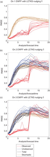
The choice of κ when we use the LETKS as a relaxation within the EWPF is a complicated and not fully understood process. Figures B1–B4 in the Appendix show the behaviour of the analysis as you vary κ for each different observation network. What is clear is that the optimal κ is problem dependent. Further, it can be seen that κ=1 performs poorly in all cases. One conjecture for this is that using the LETKS as a relaxation gives a large change to some ensemble members. Making a large change to the position of any ensemble member must be paid for in the weights of that particle: its weight decreases. Keeping κ=1 forces all ensemble members to degrade their positions in order to achieve a weight equal to that of the worst particle. This process could then move all the other ensemble members away from the truth – thus increasing the RMSE. Further investigations on this matter are warranted.

8. Conclusions

Both the LETKF and the EWPF were used in data assimilation experiments with the BV model. Typical values for the parameters in the methods were used for three different set of observations.

In all cases, the LETKF was found to give RMSEs that were substantially smaller than those achieved by the EWPF. Notably, the EWPF gives RMSEs much larger than that of the observation error standard deviations.

The efficacy of the EWPF to minimise the RMSE was shown to be controlled by the nudging stage of the method. Experiments with both simple nudging and using the LETKS as a relaxation showed that the resulting particle filter followed those trajectories closely. An analysis of the relaxation term used in the simple nudging procedure showed why such a method does not bring the ensemble mean close to the truth. This same analysis motivated the use of the LETKS relaxation and this was numerically shown to lead to improvements in RMSE.

The model investigated had a state dimension of N _x =262 144 and assimilated N _y =65 536 observations at each analysis. In such a high-dimensional system, it is a challenge to ascertain if the posterior is non-Gaussian. Without such knowledge it appears that the LETKF is a better method of data assimilation in terms of efficiency and accuracy.

Finally, note that all these experiments were conducted with an ensemble size of N _e =48. This ensemble size is representative of what can typically be run operationally. In the future, if much larger ensembles are affordable, then the results presented here may be different when the data assimilation methods are tuned to a significantly larger ensemble size.

Fig. A1 Performance of the EWPF under different parameters.

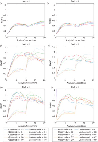
Fig. B1 Performance of the EWPF with the LETKS relaxation when κ=1.0.

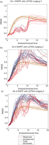
Fig. B2 Performance of the EWPF with the LETKS relaxation when κ=0.75.

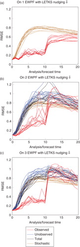
Fig. B3 Performance of the EWPF with the LETKS relaxation when κ=0.50.

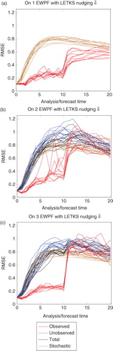
Fig. B4 Performance of the EWPF with the LETKS relaxation when κ=0.25.

9. Acknowledgements

The author would like to thank Chris Snyder for his insightful questioning into the effectiveness of the EWPF and Keith Haines for his questions regarding the practical implementation of the EWPF within a re-analysis system. Both lines of inquiry showed the need to perform the investigations in this article.

The author would also like to thank Javier Amezcua and Peter Jan van Leeuwen for their valuable discussions.

This work was supported by NERC grant NE/J005878/1. This work used the ARCHER UK National Supercomputing Service (www.archer.ac.uk).

10. Appendix

Appendix A: EWPF parameter sensitivity

Appendix B: EWPF with LETKS relaxation

References

- Ades M. , van Leeuwen P . An exploration of the equivalent weights particle filter. Q. J. R. Meteorol. Soc. 2013; 139(672): 820–840.
- Ades M. , van Leeuwen P . The equivalent-weights particle filter in a high dimensional system. Q. J. R. Meteorol. Soc. 2015; 141(687): 484–503.
- Anderson J. L. , Anderson S. L . A Monte Carlo implementation of the nonlinear filtering problem to produce ensemble assimilations and forecasts. Mon. Weather. Rev. 1999; 127(12): 2741–2758.
- Baker J. E . Reducing bias and inefficiency in the selection algorithms. Proceedings of the Second International Conference on Genetic Algorithms and their Application. 1987; NJ, Lawrence Erlbaum Associates: Hillsdale. 14–21.
- Baker L. H. , Rudd A. C. , Migliorini S. , Bannister R. N . Representation of model error in a convective-scale ensemble prediction system. Nonlinear Processes Geophys. 2014; 21(1): 19–39.
- Bayes T. , Price R . An essay towards solving a problem in the doctrine of chances. By the late Rev. Mr. Bayes, F.R.S Communicated by Mr. Price, in a letter to John Canton, A.M.F.R.S. Phil. Trans. 1763; 53: 370–418.
- Bishop C. H. , Etherton B. J. , Majumdar S. J . Adaptive sampling with the ensemble transform Kalman filter. Part I: theoretical aspects. Mon. Weather Rev. 2001; 129(3): 420–436.
- Browne P. A. , van Leeuwen P. J . Twin experiments with the equivalent weights particle filter and HadCM3. Q. J. R. Meteorol. Soc. 2015; 141: 3399–3414. 693 October 2015 Part B.
- Browne P. A. , Wilson S . A simple method for integrating a complex model into an ensemble data assimilation system using MPI. Environ. Model. Software. 2015; 68: 122–128.
- Burgers G. , Jan van Leeuwen P. , Evensen G . Analysis scheme in the ensemble Kalman filter. Mon. Weather Rev. 1998; 126(6): 1719–1724.
- Charney J. G. , Fjörtoft R. , von Neumann J . Numerical integration of the barotropic vorticity equation. Tellus A. 1950; 2(4): 238–254.
- Chorin A. J. , Tu X . Implicit sampling for particle filters. Proc. Natl. Acad. Sci. USA. 2009; 106(41): 17249–17254.
- Dashti M. , Law K. J. H. , Stuart A. M. , Voss J . MAP estimators and their consistency in Bayesian nonparametric inverse problems. Inverse Probl. 2013; 29(9): 095017.
- Doucet A. , de Freitas N. , Gordon N . Sequential Monte Carlo Methods in Practice. Series Statistics For Engineering and Information Science. 2001. Springer, New York.
- Evensen G . Sequential data assimilation with a nonlinear quasi-geostrophic model using Monte Carlo methods to forecast error statistics. J. Geophys. Res. 1994; 99(C5): 10143–10162.
- Evensen G . Data Assimilation. 2007; Berlin Heidelberg: Springer.
- Gordon N. , Salmond D. , Smith A . Novel approach to nonlinear/non-Gaussian Bayesian state estimation. IEE Proc. F (Radar and Signal Processing). 1993; 140: 107–113.
- Hunt B. R. , Kostelich E. J. , Szunyogh I . Efficient data assimilation for spatiotemporal chaos: a local ensemble transform Kalman filter. Physica D. 2007; 230(1–2): 112–126.
- Jazwinski A. H . Stochastic Processes and Filtering Theory. 1970; Academic Press, New York & London.
- Kalman R. E . A New Approach to Linear Filtering and Prediction Problems. Journal of Basic Engineering. 1960; 82(1): 35.
- Klaas M. , de Freitas N. , Doucet A . Toward practical N 2 Monte Carlo: the marginal particle filter. Proceedings of the Twenty-First Annual Conference on Uncertainty in Artificial Intelligence (UAI-05). 2005; Arlington, Virginia: AUAI Press. 308–315.
- Krishnamurti T. , Bedi H. , Hardiker V. , Watson-Ramaswamy L . An Introduction to Global Spectral Modeling. 2006; Springer, New York: Atmospheric and Oceanographic Sciences Library.
- Le Dimet F. X. , Talagrand O . Variational algorithms for analysis and assimilation of meteorological observations: theoretical aspects. Tellus A. 1986; 38A(2): 97–110.
- Lei J. , Bickel P. , Snyder C . Comparison of ensemble Kalman filters under non-Gaussianity. Mon. Weather Rev. 2010; 138(4): 1293–1306.
- Posselt D. J. , Bishop C. H . Nonlinear parameter estimation: comparison of an ensemble Kalman smoother with a Markov chain Monte Carlo algorithm. Mon. Weather Rev. 2012; 140(6): 1957–1974.
- Snyder C. , Bengtsson T. , Bickel P. , Anderson J . Obstacles to high-dimensional particle filtering. Mon. Weather Rev. 2008; 136(12): 4629–4640.
- Tennant W. J. , Shutts G. J. , Arribas A. , Thompson S. A . Using a stochastic kinetic energy backscatter scheme to improve MOGREPS probabilistic forecast skill. Mon. Weather Rev. 2011; 139: 1190–1206.
- Tippett M. K. , Anderson J. L. , Bishop C. H. , Hamill T. M. , Whitaker J. S . Ensemble square root filters. Mon. Weather Rev. 2003; 131(7): 1485–1490.
- van Leeuwen P . Nonlinear data assimilation in geosciences: an extremely efficient particle filter. Q. J. R. Meteorol. Soc. 2010; 136(653): 1991–1999.
- van Leeuwen P. J . Particle filtering in geophysical systems. Mon. Weather Rev. 2009; 137(12): 4089–4114.
- Wang X. , Bishop C. H. , Julier S. J . Which is better, an ensemble of positive-negative pairs or a centered spherical simplex ensemble?. Mon. Weather Rev. 2004; 132: 1590–1605.
- Zhu M. , Leeuwen P. J. V. , Amezcua J . Implicit equal-weights particle filter. Q. J. R. Meteorol. Soc. 2016; 142: 1904–1919.