Long-term changes in the seasonality of Baltic sea level

Abstract

The seasonal cycle accounts for about 40% of the total sea level variability in the Baltic Sea. In a climate change context, changes are expected to occur, not only in mean levels but also in the seasonal characteristics of sea level. The present study addresses the quantification of changes in the seasonal cycle of sea level from a set of century-long tide gauge records in the Baltic Sea. In order to obtain robust estimates of the changes in amplitude and phase of the seasonal cycle, we apply different methods, including continuous wavelet filtering, multi-resolution decomposition based on the maximal overlap discrete wavelet transform, auto-regressive-based decomposition, singular spectrum analysis and empirical mode decomposition. The results show that all methods generally trace a similar long-term variability of the annual cycle amplitudes, and we focus on discrete wavelet analysis as the natural counterpart of classical moving Fourier analysis. In contrast to previous studies suggesting the existence of long-term changes in the seasonal cycle, in particular an increase of the annual amplitude, we find alternating periods of high and low amplitudes without any clear indication of systematic long-term trends. The derived seasonal patterns are spatially coherent, discriminating the stations in the Baltic entrance from the remaining stations in the Baltic basin, for which zonal wind accounts for typically more than 40% of the variations in amplitude.

• sea level
• Baltic Sea
• seasonality
• wavelet transform

1. Introduction

The seasonal cycle is a ubiquitous feature of climate records in general, and sea level records in particular. In the Baltic Sea, the seasonal cycle of sea level is a well-known feature, with a pronounced minimum in spring (e.g. Ekman and Stigebrandt, 1990). Although much attention has been focused on long-term variability in the mean and trends associated with climate variability (e.g. Samuelsson and Stigebrandt, 1996; Ekman, 1999; Johansson et al., 2001; Hünicke and Zorita, 2006; Barbosa, 2008; Donner et al., 2012) changes in seasonality are equally relevant.

Previous studies have suggested an increase in the amplitude of the seasonal sea level cycle in the Baltic Sea. Ekman and Stigebrandt (1990) found an increase in the seasonal amplitude from 7 to nearly 11 cm applying Fourier analysis to two distinct 80-yr periods of the Stockholm record. Plag and Tsimplis (1999) applied a moving harmonic analysis over time windows of fixed length (19 yr) and found over the North Sea and Baltic area regionally coherent temporal variability of the annual and semi-annual cycles and an increase in amplitude in the last decades of the 20th century. Hünicke and Zorita (2008) assumed the shape of the seasonal cycle to be constant, with a minimum in spring and a maximum in winter, and estimated linear trends for the difference between averaged sea level in winter and in the previous spring, detecting significant trends in this amplitude. Medvedev (2014) analysed the temporal variability of the seasonal cycle of sea level using classical harmonic analysis applied to yearly series, observing significant changes in seasonal amplitudes from year-to-year, and seasonal fluctuations to be caused by the zonal wind component.

The aforementioned studies have limitations from the methodological point of view, such as the use of arbitrarily fixed size time windows or the underlying assumption of a cycle with the same profile every year. Furthermore, while agreeing upon the non-constancy of the seasonal cycle of sea level in the Baltic Sea, different physical origins for that change have been proposed and remain to be resolved (Hünicke et al., 2015).

The present study examines changes in the annual cycle of sea level in the Baltic Sea from long tide gauge records extending from 1900 up to the first decade of the 21st century (2012), using modern methods able to provide a flexible and detailed description of changes in the seasonality of sea level, including continuous and discrete wavelet analysis (DWT), singular spectrum analysis (SSA), auto-regressive decomposition and empirical mode decomposition (EMD). The same methods are also applied to meteorological variables in order to investigate the physical mechanisms that could explain the variability in the seasonality of Baltic sea level.

The remainder of this paper is organised as follows: The tide gauge records analysed in this work are described in Section 2. Section 3 introduces the different methods applied for extracting the seasonal cycle of sea level. The derived seasonal components are presented in Section 4 and further discussed in Section 5. Concluding remarks are given in Section 6.

2. Data

Monthly tide gauge records from the Baltic Sea were obtained from the Permanent Service for Mean Sea Level (PSMSL, Woodworth and Player, 2003). The criteria applied for station selection were data availability in the PSMSL database for the period 1900–2012 and completeness of the record (less than 2.5% missing values). The latter criterion implies disregarding some existing even longer-term records of Baltic sea level like the Kronstadt tide gauge (Bogdanov et al., 2000) and results in a final data set of nine long tide gauge records (Table 1, Fig. 1). In the case of the Gedser and Hornbæk records (Hansen, 2007), with 13 and 29 missing months, respectively, the Holt–Winters method (Holt, 1957; Winters, 1960) was applied for gap-filling as in Barbosa and Silva (2009). All other records have less than four missing months over the whole 113-yr period, and these were linearly interpolated.

Fig. 1 Map with the locations of the tide gauge stations in the Baltic Sea (°) and grid points of 20th century reanalysis (⋄) and ERA-Interim reanalysis (⋆).

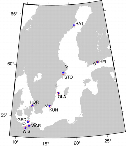
Table 1. Analysed monthly tide gauge records (1900–2012)

Station name	Lon. (°E)	Lat. (°N)	Missing values (%)
Wismar (WIS)	11.46	53.90	0.15
Warnemünde (WAR)	12.10	54.17	0.15
Gedser (GED)	11.93	54.57	0.98
Hornbæk (HOR)	12.46	56.10	2.18
Kungsholmsfort (KUN)	15.59	56.10	0.08
Ölands Norra Udde (OLA)	17.10	57.37	0
Stockholm (STO)	18.08	59.32	0
Helsinki (HEL)	24.97	60.15	0.15
Ratan (RAT)	20.90	63.99	0.23

Since the focus of the present study is on seasonal variability, all records were linearly detrended, thereby removing any linear long-term variability associated with climate trends as well as vertical land movements due to land uplift from glacial isostatic adjustment (GIA) or to subsidence.

In order to gain insight into the physical mechanisms driving sea level variability, atmospheric reanalysis data were analysed, including monthly time series of surface pressure, air temperature (2 m), wind speed, zonal wind and meridional wind (10 m). Two distinct reanalysis data sets were considered: the 20th century reanalysis version 2 (Compo et al., 2006), extending up to the whole 20th century but with low spatial resolution (2 ° grid), and the ERA-Interim reanalysis (Dee et al., 2011) only available from 1979 onwards but with higher spatial resolution (0.125 ° grid). In both cases, the reanalysis time series were taken from the grid points closest to each tide gauge station (Fig. 1). Additionally, the PC-based index of the winter North Atlantic Oscillation (NAO) is considered since it is somewhat less noisy than station-based indices, while capturing the full spatial patterns of the NAO (Hurrel et al., 2003).

3. Methods

A wide range of methods can be applied to the study of seasonality. In the present study, five different methods are applied simultaneously rather than focusing on a single approach, based on the rationale that every method has its own range of assumptions, strengths and limitations and there is not a single method that is optimal for each and every case. Since the focus here is on the analysis of the temporal variability of the seasonal cycle, the methods need to be flexible enough to allow for a time-varying description of the seasonal cycle (including changes in the amplitude, phase and shape), and at the same time very robust in order to extract significant features and reduce eventual artefacts. Such requirements are not met by many traditional methods (including classical time series decomposition in the time domain and moving harmonic analysis in the frequency domain). Classical decomposition, being based on moving averages, lacks robustness. Its results also strongly depend on parameters that are arbitrarily set, in a trade-off between goodness-of-fit and smoothness. In turn, moving harmonic analysis is based on arbitrarily pre-defined windows and assumes a fixed (sinusoidal) shape for the seasonal cycle.

In this work, a set of modern methods is considered that are able to extract flexible and robust time-varying periodic signals. This selection aims to be representative of the different types of methods that could be used for that purpose and reflects a naturally biased judgement of the methods that appear adequate for the analysis of the seasonal cycle. Wavelet methods are a very flexible alternative to classical frequency domain techniques in the case of non-stationary signals and will be addressed in Section 3.1. Auto-regressive decomposition (Section 3.2) is a model-based approach very effective for the description of time-varying periodic patterns, while being considerably simpler than other recent time-domain modelling approaches such as dynamic linear models or structural time series models (e.g. Harvey, 1990; West and Harrison, 1997). SSA (Section 3.3) is a flexible non-parametric approach for the description of the dynamic components of a time series, including the seasonal cycle. Finally, EMD (Section 3.4) is a completely data-driven approach yielding a decomposition following very closely the temporal structure of the time series.

3.1. Wavelet analysis

Wavelet analysis is particularly advantageous for the analysis of non-stationary signals due to its inherent localisation in both time and frequency. Given their complementary nature, in the present study both continuous and discrete basis functions will be considered, as detailed in Sections 3.1.1 and 3.1.2, respectively.

3.1.1. Continuous wavelet transform.

The continuous wavelet transform (CWT) provides a generalisation of classical (Fourier transform-based) spectral analysis that allows unfolding a time series simultaneously into time and frequency domain. Specifically, the CWT can be mathematically represented as the convolution of the observed signal with some function (the so-called mother wavelet) that exhibits localised oscillations and can be shifted and rescaled in time by continuously varying just two parameters. In this spirit, if the shift and scale parameters of the mother wavelet are chosen such that it coincides locally with some oscillation of the signal under study, the squared modulus of the convolution will have high values.

Here, we use a complex Morlet wavelet, which is defined as a complex exponential function with an exponentially decaying envelope of Gaussian shape and is frequently used in geophysical applications (Torrence and Compo, 1998). Specifically, we fix the scale of the mother wavelet to 12 months, implying that we are not interested in a full unfolding of the signal in the time-frequency domain, but use CWT as a filtering technique for obtaining the seasonal cycle of our sea level records. We emphasise that this restriction is justified since we are interested in a variability component of fixed periodicity, but possibly varying phasing. The latter can be obtained from considering the angle spanned by both real and imaginary part of the CWT. In this spirit, the CWT framework is different from the other techniques detailed below in that it (1) does not provide a simple additive decomposition of the records into a fixed number of variability modes and (2) directly provides amplitude (CWT modulus) and phase (CWT phase) information related to the seasonal cycle.

3.1.2. Discrete wavelet transform.

The DWT is particularly appropriate for the analysis of time series exhibiting variability on a multitude of time-scales (Percival and Walden, 2000). The Maximal Overlap Discrete Wavelet Transform [MODWT, Percival and Mojfeld (1997)] is computationally more expensive but has the advantage over the classical DWT of working with time series of any (i.e. not necessarily dyadic) length. The MODWT of level J ₀ of a time series X _t of length N and sampling rate Δ _t is a non-orthogonal transform yielding an additive decomposition into J ₀ detail sub-series associated to band-pass filtered series with approximate pass-band (1/2 ^j+1)Δ _t ≤f≤(1/2 ^j )Δ _t (j=1,…,J ₀), and a remainder smooth sub-series reflecting long term changes . The MODWT also yields a scale-by-scale decomposition of variance, breaking up the variance of X _t into J ₀ components, and allowing to summarise the information in the corresponding spectral density function by a single value per band. The level of the decomposition (J ₀) is selected taking into account the goals of the analysis, with the constraint J ₀≤log₂(N). For a detailed review of DWT including geophysical applications, see Percival (2008).

3.2. Auto-regressive-based (AR) decomposition

From the dynamic linear representation of an auto-regressive process demonstrated by West (1997), any auto-regressive process describing a time series as a linear combination of values at previous times t−1, t−2,…, t−p can be written as the sum of p components. Furthermore, each of these p components is either an auto-regressive process itself of order p=1, corresponding to a trend component, or an auto-regressive process of order 2, corresponding to a periodic component. This allows to decompose a time series into time-varying oscillatory components and long-term components akin to the first-order linear decomposition of a system's dynamics in classical physics. For further details on the method and applications to sea level time series, see Barbosa et al. (2008).

3.3. Singular spectrum analysis

SSA provides an additive decomposition of a time series into pairwise orthogonal (i.e. linearly independent) variability patterns (Broomhead and King, 1986) based on the classical idea of empirical orthogonal function (EOF) or principal component analysis [PCA, Preisendorfer (1988)]. For this purpose, SSA first unfolds the given record into a multivariate time series by considering a number M of subsequently lagged replications of the original data. In a second step, PCA is applied to this data set. Then, the leading modes of the resulting decomposition correspond to the main regular variability patterns of the record under study. One main advantage of this approach is its general flexibility in terms of time-varying amplitudes and phases of possible oscillatory signals, since the underlying frequency is not predetermined, but follows as a result of the analysis.

In the present case, we use M=25 copies of the studied time series shifted by 1 month each, thus accounting for a maximum time shift of 24 months between the component series used in the PCA step. Since this maximum delay corresponds to twice the oscillation period of interest (12 months), this setting is appropriate for identifying seasonal variability components.

3.4. Empirical mode decomposition

As a potentially even more data-adaptive method than SSA, we finally consider (EMD, Huang et al., 1998), which provides another approach to obtaining an additive decomposition of time series into multiple components. Unlike the approaches discussed above, EMD cannot be represented by analytical transformations of the data, but is defined in an algorithmic way. Specifically, the resulting variability modes (intrinsic mode functions, IMFs) result from an iterative computation of the upper and lower envelopes of the signal, the mean of which represent the IMFs that are subsequently removed from the data. In the context of the present work, the high flexibility of EMD, however, might be problematic, since the individual IMFs are not bound to specific frequencies or frequency bands, but may exhibit crossover phenomena (known as the mode mixing problem) potentially prohibiting the unique association of the seasonal cycle to just a single IMF. We will get back to this question in Section 4.1.

4. Results

The seasonal cycle of sea level in the Baltic Sea is slightly asymmetric including both annual and semi-annual variability, as known since the early 20th century (Ekman, 2009). The mean seasonal cycle resulting from averaging monthly observations over the whole period and representing both yearly and half-yearly components is first considered in Section 4.1. Then, the seasonal cycle patterns obtained with the different methods described in Section 3 are compared in Section 4.2. The interannual changes in the annual amplitudes and phases are detailed in Section 4.3.

4.1. Mean seasonal cycle

The mean seasonal cycle is computed for each monthly tide gauge record by averaging the values for each calendar month. Figure 2 shows the mean seasonal cycle over the complete period 1900–2012, while the mean seasonal cycle for the 1979–2012 period concurrent with high-quality atmospheric reanalysis data is displayed in Fig. 3. The vertical bars represent the standard deviation associated to each monthly mean value. The results for the two periods are qualitatively similar, with the mean seasonal cycle exhibiting a minimum in spring and a maximum in autumn at all stations. The mean seasonal pattern exhibits a clear latitudinal dependence with the amplitude increasing northward, in agreement with previous work (Ekman, 1996). Minima occur earlier (in March) for the southernmost stations (Wismar, Warnemünde) and later (typically May) for the remaining stations. The maxima occur in late summer (August/September) in the southern stations and in winter (December/January) at the remaining tide gauges.

Fig. 2 Mean seasonal cycle (1900–2012) and associated standard deviation computed for each tide gauge station (solid line) and estimated by linear regression from 20th century reanalysis atmospheric parameters (dashed line).

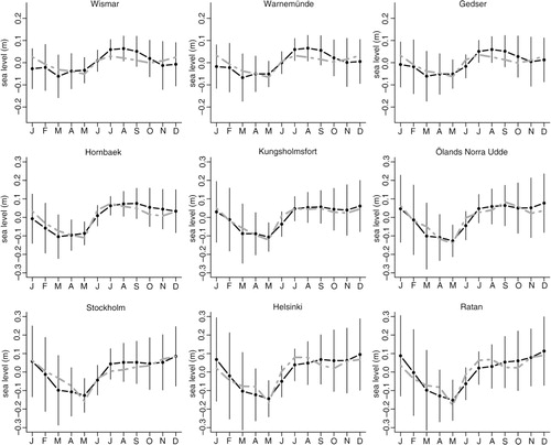
Fig. 3 As in Fig. 2 for the period 1979–2012 using atmospheric parameters from the ERA-Interim reanalysis.

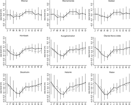
The seasonal variability of sea level in the Baltic Sea is strongly determined by atmospheric conditions, including the direction of prevailing winds influencing the water exchange at the Baltic entrance, and the atmospheric pressure via a direct inverse barometric response (e.g. Ekman, 1998; Andersson, 2002). In order to quantify the influence of atmospheric parameters in the mean seasonal cycle of Baltic sea level, the mean seasonal cycle is also computed for the reanalysis parameters [surface pressure, air temperature (2 m), wind speed (10 m) and zonal and meridional wind components (10 m)]. Then, a simple linear regression model is considered, relating the mean seasonal cycle of sea level and the seasonal pattern of each individual atmospheric parameter. For each location the dominant atmospheric variable is selected corresponding to the single-predictor model explaining a highest fraction of seasonal variability, given by the adjusted coefficient of determination (adjusted R ²). The mean seasonal cycles derived from the linear regressions are represented in Figs. 2 and 3 (dashed lines) for the complete and the 30-yr period, respectively. The regression models are summarised in Table 2 for the complete 1900–2012 period, based on the 20th century reanalysis, and for the 1979–2012 period, based on the ERA-Interim reanalysis. Furthermore, the results obtained with the 20th century reanalysis restricted to the 1979–2012 period common to the two models are also presented.

Table 2. Linear regression models for the mean seasonal cycle of sea level and reanalysis atmospheric parameters

	20th century 1900–2012		20th century 1979–2012		ERA-interim 1979–2012
Station	Model	Adj. R ^2 (%)	R ^2 Model	Adj. R ^2 (%)	Model	Adj. R ^2 (%)
WIS	u-wind	38	air T	28	air T	30
WAR	u-wind	53	u-wind	35	u-wind	30
GED	u-wind	59	u-wind	43	u-wind	50
HOR	u-wind	82	u-wind	68	u-wind	46
KUN	u-wind	89	u-wind	845	u-wind	80
OLA	u-wind	85	u-wind	87	u-wind	87
STO	Pressure	81	Pressure	87	u-wind	84
HEL	Pressure	79	Pressure	79	Pressure	61
RAT	Pressure	80	u-wind	83	u-wind	84

Taking the complete 20th century period, the mean seasonal cycle of atmospheric parameters is able to explain a substantial fraction of the variation of the mean seasonal cycle (typically more than 50%) as shown by the adjusted R ² in Table 2. This percentage is usually lower when restricting the 20th century reanalysis to the 1979–2012 subset as a result of a less smooth curve describing the mean seasonal cycle for the shorter period, particularly for the stations at the Baltic entrance (WIS, WAR, GED). For the 1900–2012 period the zonal wind is the dominant atmospheric variable except for the northernmost stations (STO, HEL, RAT) for which it is replaced by atmospheric pressure. The results based on the 20th century reanalysis for the two distinct periods are very similar except for the southernmost station, WIS, for which air temperature becomes the main covariate, and for the northernmost station, RAT, with atmospheric pressure being replaced by the zonal wind. This change for the WIS and RAT stations in the most recent period is consistent with the ERA-Interim results for the same period. The only difference between the 20th century and ERA-interim reanalysis for the common 1979–2012 period is for the Stockholm station, with atmospheric pressure replaced by zonal wind in the ERA-Interim case, possibly reflecting the distinct spatial scales associated with the two reanalysis models. Furthermore, note that atmospheric pressure and zonal wind are not independent variables and both can explain a significant fraction of the mean seasonal cycle.

The atmospheric parameters typically explain 28–59% of the variability for the southernmost stations (WIS, WAR and GED) and more than 60% for the remaining stations. The difficulty in modelling the mean seasonal cycle of sea level for the stations at the Baltic entrance reflects the complex geographical setting of the area and the influence of non-atmospheric factors associated with the exchange of water with the North Sea, such as salinity. For all stations larger deviations between the modelled and actual mean seasonal cycles occur in March and July–October. A possible explanation is related with the role played in the mean seasonal cycle of sea level by non-atmospheric drivers such as sea ice-cover (which has a maximum in February–March) or hydrological factors (river run-off and freshwater discharge, precipitation), which are important especially during summer.

4.2. Variations in seasonal cycle: method intercomparison

The seasonal sea level cycle derived with the different methods described in Section 3 is illustrated for the Stockholm record in Fig. 4. The seasonal cycle from the CWT (Fig. 4a) is obtained by extracting the signal corresponding to a fixed frequency of 1 cycle/yr. The discrete counterpart of the CWT yields a signal decomposition into discrete scales of variability. MODWT is applied up to a decomposition level J ₀=4 using a Daubechies least-asymmetric (LA) filter of width L=8 months (Daubechies, 1988), and the seasonal component is obtained from the level j=3 component, associated with scales from 8 to 16 months (Fig. 4b). The seasonal component from auto-regressive decomposition (Fig. 4c) is extracted as the resulting periodic component with a period of 12 months. In the case of SSA, the seasonal cycle is represented by the two largest eigenvalues of the covariance matrix associated with the lagged observations, which have similar magnitude as required for the reconstruction of oscillatory signals (with the two components taking the role of sine and cosine functions in classical harmonic decomposition). Finally, EMD reveals one component (IMF-3) with variability confined to the seasonal scale; thus, this component is used as a proxy for the seasonal cycle.

Fig. 4 Seasonal sea level cycle at Stockholm derived by (a) continuous wavelet transform (CWT), (b) discrete wavelet transform (DWT), (c) auto-regressive-based decomposition (AR), (d) singular spectrum analysis (SSA) and (e) empirical mode decomposition (EMD).

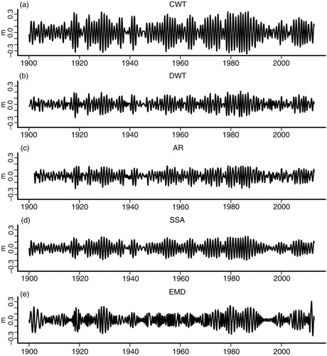
Figure 4 shows that the seasonal sea level cycle exhibits considerable temporal changes, with periods of strong seasonal variability especially around 1930, 1955 (not seen by EMD) and between 1970 and 1990 (with some interruption between 1975 and 1978), but also for some other shorter periods of time, as well as periods of very weak, almost absent, seasonal cycle (especially in the 1940s and 1990s to 2000s). The different methods yield qualitatively consistent estimates in terms of coherent periods of high (low) seasonal variability being simultaneously identified by the different approaches. The CWT cycle has, however, a larger amplitude than the ones inferred by the other methods, since CWT provides a filtering rather than a time-scale decomposition (i.e. possible compensatory effects of nearby frequencies are absent). In turn, the seasonal cycle from EMD is more irregular and less similar to the components from the other methods, which probably results from the lower frequency stability of this method. Despite being totally unrelated methods, based on completely distinct assumptions, the results from the DWT, AR and SSA methods are very similar, giving confidence in the significance of the derived patterns. Hereafter, the seasonal cycles derived from the DWT method will be considered, as the natural counterpart of the classical moving harmonic analysis approach.

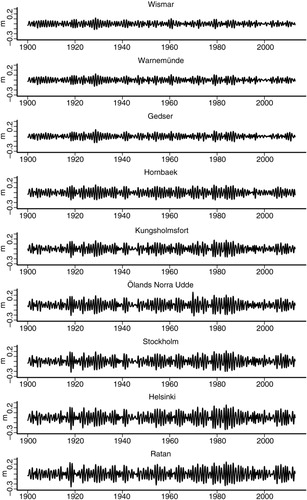
The seasonal components obtained from the DWT decomposition for all records are shown in Fig. 5. The long-term changes of seasonal cycle amplitudes (see Section 4.3 for a more detailed discussion) exhibit considerable geographical coherence, with very similar variability at the seasonal scale for the different stations. Warnemünde, Wismar and Gedser exhibit a very similar and relatively low-amplitude seasonal cycle variability, while Hornbæk displays an intermediate seasonal pattern between the southernmost and the remaining stations in the central and northern Baltic Sea, where the overall amplitudes of the seasonal cycle are significantly larger.

Fig. 5 Seasonal sea level cycle estimated by the DWT method.

4.3. Interannual changes of annual amplitudes and phases

In the following, the seasonal variability of Baltic sea level is represented by the yearly amplitude (the difference between the maximum and minimum value of the seasonal cycle for each calendar year) and the phase (here represented by the months of occurrence of the maximum and minimum sea level for each year).

The amplitude of the seasonal cycle derived by discrete wavelet decomposition is shown in Fig. 6. The time series of annual amplitudes display long-term variability with alternating periods of high and low amplitudes. Linear trends are not statistically significant. The annual amplitudes exhibit a high degree of spatial consistency characterised by two distinct interannual variability patterns separating the southern stations at the Baltic entrance from the remaining locations (again, Hornbæk displays a somewhat intermediate behaviour).

Fig. 6 Seasonal cycle amplitude estimated from the DWT method.

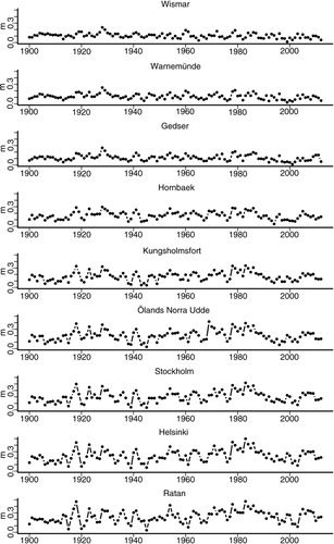
In order to examine the origin of the interannual changes in the annual amplitude of sea level, a comparison is performed with the annual amplitudes of atmospheric pressure and winds (derived in exactly the same way as for sea level) as well as with the NAO index, which is known to strongly influence atmospheric circulation and sea level variability in the Baltic Sea (e.g. Ekman, 2003; Jevrejeva et al., 2005; Bastos et al. 2013). The corresponding linear regression models (same approach as before) for the complete 1900–2012 period and the 1979–2012 period are summarised in Table 3. The results show a very poor performance of the models for the stations in the Baltic entrance, particularly WIS, confirming the inability of atmospheric parameters alone to explain the variability in the amplitude of the seasonal cycle for these stations. However, the models show some consistency between the two reanalyses for the common 1979–2012 period, with air temperature at WIS and the NAO at WAR and GED explaining more than 10% of the changes in annual amplitude. For the remaining stations the results based on the same 20th century reanalysis model for the complete and shorter period are very similar. The ERA-Interim results are different for STO and HEL, with atmospheric pressure replaced by zonal wind, likely as a result of the smaller spatial scale of the ERA-Interim reanalysis. Note again that pressure, zonal wind and the state of the NAO are not independent variables, hindering the interpretation of the role played by each factor. Except for the northernmost station (RAT) for which the contribution of pressure is dominant, the variations in the annual amplitude of sea level for the tide gauges in the Baltic basin (KUN, OLA, STO, HEL) and for HOR are correlated with the zonal wind, which explains typically about 40% of the amplitude variations.

Table 3. Linear regression models for the interannual changes in the annual amplitude of sea level and reanalysis atmospheric parameters

	20th century 1900–2012		20th century 1979–2012		ERA-interim 1979–2012
Station	Model	Adj. R ^2 (%)	Model	Adj. R ^2 (%)	Model	Adj. R ^2 (%)
WIS	NAO	2	air T	12	air T	14
WAR	u-wind	9	NAO	13	NAO	13
GED	u-wind	17	NAO	17	NAO	17
HOR	u-wind	58	u-wind	51	u-wind	42
KUN	u-wind	65	u-wind	62	u-wind	51
OLA	u-wind	46	u-wind	44	u-wind	35
STO	Pressure	43	Pressure	35	u-wind	46
HEL	Pressure	53	Pressure	52	u-wind	31
RAT	Pressure	48	Pressure	47	Pressure	30

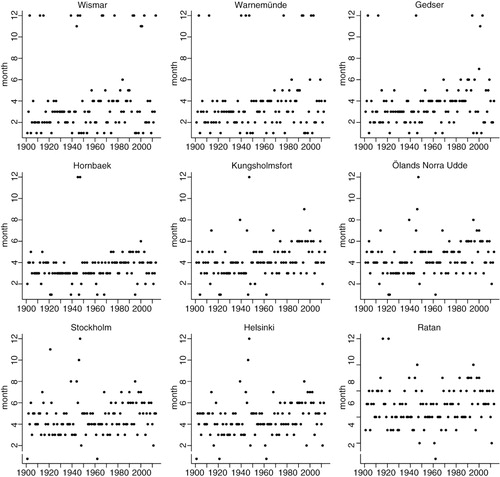
The phase of the seasonal cycle is studied in terms of the months of occurrence of the maximum and minimum for each calendar year. Figures 7 and 8 show the time series of the timings of the yearly maxima and minima, respectively, of the seasonal cycles derived by DWT. The annual phase is mostly stable in time, with the larger differences in phase observed for some calendar years corresponding to years with almost absent seasonal cycle for which the phase is less well-defined. The annual phase for the stations away from the Baltic entrance (KUN, OLA, STO, HEL, RAT) shows after the 1990s a tendency for maxima to occur later (in December–January), consistent with Ekman (1998) who concluded from the analysis of the Stockholm record that winter plays a central role in the seasonal variability of sea level, leading to a shift of the maximum from July to August to December.

Fig. 7 Yearly seasonal cycle maximum estimated from the DWT method.

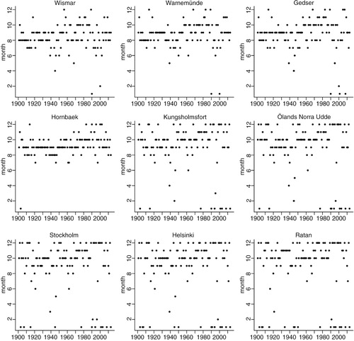
Fig. 8 Yearly seasonal cycle minimum estimated from the DWT method.

5. Discussion

Before discussing the general shape and long-term changes of the seasonal cycle in Baltic sea level inferred using the different methods introduced in Section 3, we emphasise the necessity of discussing the separability of this variability component.

On the one hand, in this work we only consider the seasonal cycle in the mean sea level, disregarding the fact that the interannual variability of sea level may also show a variance (and even higher-order moments) exhibiting seasonal fluctuations. In the underlying sea level records, such behaviour might be represented in terms of heteroskedasticity, i.e. a variance depending on mean sea level. We shall not further discuss this question here, but leave a detailed investigation and discussion of temporal changes in the full distribution of sea level for each calendar month or season as a problem for future work. Notably, one closely related and practically relevant aspect would be tracing changes in seasonal extremes as compared to possible trends in mean seasonal sea level, thereby extending our previous works on trends in sea level extremes (Donner et al., 2012; Ribeiro et al., 2014) in the Baltic by a seasonal resolution. However, it appears reasonable to focus such an investigation on daily rather than monthly mean sea level, which restricts the number of available high-quality long-term data sets even further.

On the other hand, an important aspect directly related to this work is how well the different methods are able to extract variability components that can actually be identified with the seasonal cycle of Baltic sea level. For the two wavelet-based approaches, this is guaranteed by definition, since (1) CWT is used here as a filtering technique specifically tailored to a 12-month period in the data, whereas (2) DWT decomposes the signal into variability components the frequency bands of which are fixed. This means that the DWT mode containing the seasonal cycle also includes variability on time-scales around 12 months (i.e. 8–16 months), which appears reasonable since we are explicitly interested in interannual and long-term variations of the seasonal cycle. For illustrative purposes, Fig. 9 displays the full DWT decomposition of the tide gauge record of Stockholm into four detail components from short (2–4 months) to interannual (16–32 months) scales and a remainder smooth (long-term) component. The corresponding variance decomposition on the same four levels is summarised for all records in Table 4. All stations exhibit a similar structure with high-frequency variability and annual scales explaining most of the variance of the sea level time series, semi-annual signals explaining about 30% of variance, and interannual variability explaining less than 15% of the total variance. For the southernmost stations (WIS, WAR and GED), high-frequency variability is stronger and the annual variability is weaker. HOR and KUN exhibit an intermediate behaviour with smaller high-frequency variance and larger annual variability. The remaining tide gauges display lower high-frequency variability and slightly higher variance at all other scales (semi-annual, annual and interannual).

Fig. 9 MODWT-based multi-resolution decomposition of the Stockholm record (top) into additive components from high-frequency to long term scales.

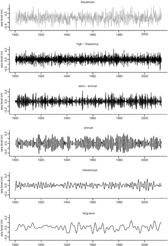
Table 4. MODWT-based variance decomposition (%)

Station	High-frequency (2–4 months)	Semi-annual (4–8 months)	Annual (8–16 months)	Interannual (16–32 months)
WIS	36	25	30	10
WAR	31	26	32	11
GED	37	26	28	10
HOR	26	22	35	11
KUN	26	28	35	11
OLA	23	28	36	12
STO	23	29	36	12
HEL	23	28	37	13
RAT	21	28	38	13

Regarding the other three methods (AR, SSA and EMD), time-scale separation is not so simply guaranteed, since specific scales are not as strictly fixed as in the case of wavelet-based methods. In this spirit, seasonality in variance and higher-order moments may actually corrupt the additive decomposition by such more flexible methods resulting in additional variability modes at periods close to 12 months, as well as harmonics and multiples of the annual period.

6. Conclusions

The mean seasonal cycle of sea level variability in the Baltic Sea is characterised by a well-defined minimum in spring and a maximum, which occurs in late summer for the southern stations (WIS, WAR, GED and HOR) and in autumn–winter for the remaining stations. Atmospheric parameters are able to explain a significant fraction of the seasonal variability in the 1900–2012 period, with winds or atmospheric pressure explaining typically 50% of the seasonal variation of sea level for the southern stations and more than 70% of the mean seasonal cycle for the other stations.

The analysis of the temporal variability of the seasonal cycle of sea level in the Baltic Sea allows identifying spatially-coherent regions, discriminating stations in the Baltic entrance (WIS, WAR and GED) from the remaining stations in the central and northern Baltic Sea (OLA, STO, HEL and RAT), with two stations (HOR and KUN) displaying an intermediate behaviour between these two groups.

The different methods applied in this study to obtain a time-varying representation of the seasonal cycle of sea level in the Baltic Sea (wavelet analysis, SSA, auto-regressive decomposition and EMD) are all able to extract a flexible description of the seasonal cycle. The diverse approaches yield a similar temporal pattern characterised by alternating periods of large seasonal amplitudes and periods of very weak, almost absent seasonal cycle. Confidence in the derived seasonal patterns is strengthened by both the similarity of results obtained by conceptually unrelated methods and the spatial coherence of the derived temporal variations.

The flexible seasonal patterns resulting from the specific methodology applied in the present study allows to examine in detail the interannual changes of annual amplitudes and phases, rather than looking into differences for arbitrarily-fixed periods. In contrast to previous studies, a systematic increase in the amplitude of the seasonal cycle is not found here. Instead, the interannual changes of seasonal cycle amplitudes are characterised by both increases and decreases, which are associated with corresponding changes in atmospheric parameters. For the stations at the Baltic entrance the interannual changes in the annual amplitude are smaller than for the other tide gauges, with the atmospheric variables explaining only a small fraction (about 10%) of the variability. For most tide gauges in the Baltic basin (HOR, KUN, OLA, STO and HEL), zonal wind alone is able to account for typically more than 40% of the interannual changes in annual amplitude over the 1979–2012 period. The fundamental role of zonal wind in the variability of the annual amplitude of sea level in the Baltic Sea documented in this study is in agreement with Medvedev (2014), who found a significant influence of the zonal wind component on seasonal fluctuations of Baltic sea level. It is also consistent with the higher coherence of sea level anomalies from satellite data with the zonal wind stress component (Stramska, 2013).

Given the unique physical and chemical characteristics of the Baltic Sea, and the relevance of seasonal variability to a wide range of biological and environmental processes, the study of seasonal changes in meteorological and oceanographic variables using flexible methods such as the ones applied in this study is of paramount relevance, particularly in a climate change context.

Acknowledgements

The presented analysis was performed with the open source software R for statistical computing and graphics and maps produced with GMT (Generic Mapping Tools). Support for the Twentieth Century Reanalysis Project dataset is provided by the U.S. Department of Energy, Office of Science Innovative and Novel Computational Impact on Theory and Experiment (DOE INCITE) program, and Office of Biological and Environmental Research (BER), and by the National Oceanic and Atmospheric Administration Climate Program Office. This work was supported by the ERDF – European Regional Development Fund through the Operational Programme for Competitiveness and Internationalisation – COMPETE 2020 Programme within project POCI-01-0145-FEDER-006961, by National Funds through the FCT, Fundação para a Ciência e a Tecnologia, as part of project UID/EEA/50014/2013 and programme IF2013, and by the German Federal Ministry for Education and Research (BMBF) via the Young Investigators Group CoSy-CC²(grant no. 01LN1306A).

References

- Andersson H . Influence of long-term regional and large-scale atmospheric circulation on the Baltic sea level. Tellus A. 2002; 54: 76–88.
- Barbosa S . Quantile trends in Baltic sea level. Geophys. Res. Lett. 2008; 35: L22704.
- Barbosa S. M. , Silva M. E . Low-frequency sea-level change in Chesapeake Bay: changing seasonality and long-term trends. Estuar. Coast. Shelf Sci. 2009; 83: 30–38.
- Barbosa S. M. , Silva M. E. , Fernandes M. J . Changing seasonality in North Atlantic coastal sea level from the analysis of long tide gauge records. Tellus A. 2008; 60: 165–177.
- Bastos A. , Trigo R. , Barbosa S. M . Discrete wavelet analysis of the influence of the North Atlantic Oscillation on Baltic Sea level. Tellus A. 2013; 65: 20077. DOI: http://dx.doi.org/10.3402/tellusa.v65i0.20077 .
- Bogdanov V. I. , Yu Medvedev M. , Solodov V. A. , Trapeznikov Y.A. , Troshkov G. A. , co-authors . Mean monthly series of sea level observations (1777–1993) at the Kronstadt gauge. Rep. Finn. Geod. Inst. 2000; 2000 1, 34pp.
- Broomhead D. S. , King G . Extracting qualitative dynamics from experimental data. Physica D. 1986; 20: 217–236.
- Compo G. P. , Whitaker J. S. , Sardeshmukh P. D . Feasibility of a 100 year reanalysis using only surface pressure data. Bull. Am. Meteorol. Soc. 2006; 87: 175–190.
- Daubechies I . Orthonormal bases of compactly supported wavelet. Commun. Pure Appl. Math. 1988; 41: 909–996.
- Dee D. P. , Uppala S. M. , Simmons A. J. , Berrisford P. , Poli P. , co-authors . The ERA-Interim reanalysis: configuration and performance of the data assimilation system. Q. J. Roy. Meteorol. Soc. 2011; 137: 553–597.
- Donner R. V. , Donner R. V. , Ehrcke R. , Barbosa S. M. , Wagner J. , co-authors . Spatial patterns of linear and nonparametric long-term trends in Baltic sea-level variability. Nonlinear Proc. Geophys. 2012; 19: 95–111.
- Ekman M . A common pattern for interannual and periodical sea level variations in the Baltic Sea and adjacent waters. Geophysica. 1996; 32: 261–272.
- Ekman M . Secular change of the seasonal sea level variation in the Baltic Sea and secular change of the winter climate. Geophysica. 1998; 34: 131–140.
- Ekman M . Climate changes detected through the world's longest sea level series. Global Planet. Change. 1999; 21: 215–224.
- Ekman M . The World's Longest Sea Level Series and a Winter Oscillation Index for Northern Europe 1774–2000. 2003; Small Publications in Historical Geophysics 12, Summer Institute for Historical Geophysics, Åland.
- Ekman M . The Changing Level of the Baltic Sea during 300 Years: A Clue to Understanding the Earth.
- Ekman M. , Stigebrandt A . Secular change of the seasonal variation in sea level and of the Pole Tide in the Baltic Sea. J. Geophys. Res. 1990; 95: 5379–5383.
- Hansen L . Hourly Values of Sea Level Observations from Two Stations in Denmark Hornbæk 1890–2005 and Gedser 1891–2005. 2007. DMI Technical Report No 07-09. DMI, Copenhagen.
- Harvey A. C . Forecasting, Structural Time Series Models and the Kalman Filter. 1990; Cambridge University Press, Cambridge.
- Holt C. C . Forecasting Seasonals and Trends by Exponentially Weighted Moving Averages. 1957; ONR Research Memorandum, 52, Carnegie Institute, Piitsburgh.
- Huang N. E. , Shen Z. , Long S. R. , Wu M. C. , Shih H. H. , co-authors . The empirical mode decomposition and the Hilbert spectrum for nonlinear and non-stationary time series analysis. Proc. Roy. Soc. Lond. A. 1998; 454: 903–995.
- Hünicke B. , Zorita E . Influence of temperature and precipitation on decadal Baltic Sea level variations in the 20th century. Tellus A. 2006; 58: 141–153.
- Hünicke B. , Zorita E . Trends in the amplitude of Baltic Sea level annual cycle. Tellus A. 2008; 60: 154–164.
- Hünicke B. , Zorita E. , Soomere T. , Madsen K. S. , Johansson M. , co-authors . Bolle H.-J . Recent change – sea level and wind waves. Second Assessment of Climate Change for the Baltic Sea Basin. 2015; Berlin: Springer. 155–185 pp.
- Hurrel J. W , Kushnir Y. , Ottersen G. , Visbeck M . The North Atlantic Oscillation: Climate Significance and Environmental Impact.
- Jevrejeva S. , Moore J. , Woodworth P. , Grinsted A . Influence of large–scale atmospheric circulation on European sea level: results based on the wavelet transform method. Tellus A. 2005; 57: 183–193.
- Johansson M. , Boman H. , Kahma K. , Launiainen J . Trends in sea level variability in the Baltic Sea. Boreal Environ. Res. 2001; 6: 159–179.
- Medvedev I. P . Seasonal fluctuations of the Baltic Sea level. Russian Meteorol. Hydrol. 2014; 39: 814–822.
- Percival D. B . Donner R. V. , Barbosa S. M . Analysis of geophysical time series using discrete wavelet transforms: an overview. Nonlinear Time Series Analysis in the Geosciences – Applications in Climatology, Geodynamics, and Solar-Terrestrial Physics. 2008; Berlin: Springer. 61–79.
- Percival D. B. , Mojfeld H . Analysis of subtidal coastal sea level fluctuations using wavelets. J. Am. Stat. Assoc. 1997; 92: 868–880.
- Percival D. B. , Walden A. T . Wavelet methods for time series analysis. 2000; Cambridge University Press, Cambridge.
- Plag H.-P. , Tsimplis M. N . Temporal variability of the seasonal sea level cycle in the North Sea and Baltic Sea in relation to climate variability. Global Planet. Change. 1999; 20: 173–203.
- Preisendorfer R. W . Principal Component Analysis in Meteorology and Oceanography. 1988; Elsevier, Amsterdam.
- Ribeiro A. , Barbosa S. M. , Scotto M. G. , Donner R. V . Changes in extreme sea-levels in the Baltic Sea. Tellus A. 2014; 66: 20921. DOI: http://dx.doi.org/10.3402/tellusa.v66i0.20921 .
- Samuelsson M. , Stigebrandt A . Main characteristics of the long-term sea level variability in the Baltic Sea. Tellus A. 1996; 48: 672–683.
- Stramska M . Temporal variability of the Baltic Sea level based on satellite observations. Estuar. Coast. Shelf Sci. 2013; 133: 244–250.
- Torrence C. , Compo G. P . A practical guide to wavelet analysis. Bull. Am. Meteorol. Soc. 1998; 79: 61–78.
- West M . Time series decomposition. Biometrika. 1997; 84: 489–494.
- West M. , Harrison P. J . Bayesian Forecasting and Dynamic Models. 1997; New York: Springer.
- Winters P. R . Forecasting sales by exponentially moving averages. Manage. Sci. 1960; 6: 324–342.
- Woodworth P. L. , Player R . The Permanent Service for Mean Sea Level: an update to the 21st century. J. Coast. Res. 2003; 19: 287–295.