Key synoptic-scale features influencing the high-impact heavy rainfall in Beijing, China, on 21 July 2012

Abstract

This work examined quantitatively the key synoptic features influencing the high-impact heavy rainfall event in Beijing, China, on 21 July 2012 using both correlation analysis based on global ensemble forecasts (from TIGGE) and a method previously used for observation targeting. The global models were able to capture the domain-averaged rainfall of >100 mm but underestimated rainfall beyond 200 mm with an apparent time lag. In this particular case, the ensemble forecasts of the National Centres for Environmental Prediction (NCEP) had apparently better performance than those of the European Centre for Medium-Range Weather Forecasts (ECMWF) and the China Meteorological Administration (CMA), likely because of their high accuracies in capturing the key synoptic features influencing the rainfall event. Linear correlation coefficients between the 24-h domain-averaged precipitation in Beijing and various variables during the rainfall were calculated based on the grand ensemble forecasts from ECMWF, NCEP and CMA. The results showed that the distribution of the precipitation was associated with the strength and the location of a mid-level trough in the westerly flow and the associated low-level low. The dominant system was the low-level low, and a stronger low with a location closer to the Beijing area was associated with heavier rainfall, likely caused by stronger low-level lifting. These relationships can be clearly seen by comparing a good member with a bad member of the grand ensemble. The importance of the trough in the westerly flow and the low-level low was further confirmed by the sensitive area identified through sensitivity analyses with conditional nonlinear optimal perturbation method.

• heavy rainfall
• sensitivity analysis
• TIGGE
• CNOP

1. Introduction

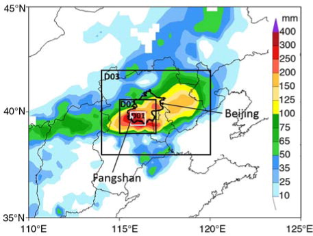
On 21 July 2012, a very heavy rainfall event occurred in Beijing, China. More than 90% of the Beijing metropolitan area was covered by >100-mm 24-h accumulated rainfall with a maximum value of 460 mm in Fangshan in southeastern Beijing, China (Fig. 1). The average rainfall over the Beijing metropolitan area reached 190 mm, the highest in the meteorological history of Beijing (Xu et al., 2012). A total of 79 people lost their lives in Beijing, mostly because of the flooding and mudslides caused by the heavy rainfall (Sun et al., 2012). The heavy rainfall caused a direct economic loss of about $1.9 billion (Sun et al., 2012).

Fig. 1 The distribution of 24-h (from 0000 UTC 21 July to 0000 UTC 22 July 2012) rainfall (shaded, mm) observation. The inner solid boxes (D01, D02 and D03) represent the three increasingly large areas used for the rainfall average.

The operational forecasts for this event were quite poor. Almost all operational deterministic forecasts underestimated the total amount of rainfall and with a 6- to 12-h lag of the beginning and peaking times of the rainfall (Xu et al., 2012; Zhang et al., 2013). Because of the large forecast error and huge amount of damage, much efforts have been made to examine the physical processes of this event. Previous studies have showed that the event could have been related to an upper-level jet, a mid-level trough, a low-level low, a low-level jet, a cold front, a landfalling tropical cyclone in south China, a monsoon low and the subtropical high (Sun et al., 2005; Chen et al., 2012; Sun et al., 2012; Yu, 2012). However, all the previous works mentioned only the weather systems that were likely involved in the occurrence of this heavy rainfall event qualitatively, so what the dominant or key synoptic features influencing this heavy rainfall were remains unknown. The capability of operational ensemble forecasts in capturing these features and the heavy rainfall has not been examined, either.

Sensitivity analysis is a common way to identify the precursors of a weather event. One way to conduct sensitivity analysis is linear correlation analysis using ensemble forecasts. Ensemble forecasts have been widely used to investigate the dynamics and predictability of weather systems. Based on ensemble sensitivity analyses, Sippel and Zhang (2008, 2010) found that the moisture condition and convective instability are important factors for tropical cyclone genesis and predictability. The European Centre for Medium-Range Weather Forecasts (ECMWF) Ensemble Prediction System (EPS) has been used to explore rainfall predictability, and the results showed that precipitation is more predictable during the winter than in the summer and rainfall associated with tropical cyclones is more predictable than the warm-season cases (Buizza et al., 1999; Mullen and Buizza, 2001; Schumacher and Davis, 2010). ECMWF EPS was also used to identify key factors influencing the May 2010 extreme rainfall in Tennessee and Kentucky (Lynch and Schumacher, 2014) and longer-term warm-season rainfall (Schumacher, 2011).

Besides correlation analysis, targeted observation methods can also be used to determine the key synoptic features that influence forecast errors. Observation targeting is a methodology in which a special area is determined within which extra observations are assimilated so that the error of a given forecast metric can be decreased the most. The weather systems in the sensitive area can be regarded as important influential systems to the examined forecast metric. Targeting strategies can be roughly classified into two groups. One is based on adjoint technology, such as singular vectors (SVs; Palmer et al., 1998); the other is ensemble-based methods, such as the ensemble transform Kalman filter (ETKF; Bishop et al., 2001). A major limitation in most of the current targeting methods, especially the adjoint strategies, is the linear error growth assumption, which may easily shift the identified target area from the true one (Reynolds and Rosmond, 2003; Huang and Meng, 2014). Mu and Duan (2003) proposed the conditional nonlinear optimal perturbation (CNOP) targeting strategy, which aims at producing the initial perturbation whose nonlinear evolution attains the maximum of a cost function under certain physical constraints over a given period. CNOP has been widely used to identify sensitive areas in observation targeting for mesoscale and tropical cyclone forecasts. The results showed that assimilating extra observations in the sensitive areas identified by CNOP had an overall positive influence on typhoon track forecasts (Mu et al., 2009; Chen, 2011; Qin and Mu, 2011; Qin et al., 2013).

The current study aims at examining the performance of global ensemble forecast guidance and identifying the dominant synoptic features influencing the high-impact heavy rainfall in Beijing, China, on 21 July 2012 using both linear ensemble correlation analyses and CNOP, an approach previously used for observation targeting. Section 2 provides an overview of the event and the data used in the study. Section 3 describes the performance of the operational forecast guidance. The results obtained from the ensemble correlation analyses are presented in Section 4, and the results obtained using CNOP are presented in Section 5. Finally, a summary and discussion are given in Section 6.

2. Data and case overview

The rainfall observations were provided by the China Meteorological Administration (CMA). They consisted of roughly 2000 rain gauge observations. The 96-h ensemble forecasts used in this work were provided by ECMWF, the National Centres for Environmental Prediction (NCEP), and CMA initialised at 0000 UTC 18 July 2012 (~72 h before the start of the rainfall) obtained from the Observing System Research and Predictability Experiment (THORPEX) Interactive Grand Global Ensemble (TIGGE; Bougeault et al., 2010) data archive. ECMWF provided a 50-member ensemble forecast with a spectral truncation of T639. NCEP had 20 members with a 1°×1° horizontal resolution. CMA had 14 members with a 0.56°×0.56° horizontal resolution. The grand ensemble, with a total of 84 members from the three NWP centres, was interpolated (by the TIGGE portal) into a common 0.5°×0.5° horizontal grid for the sensitivity analyses. Precipitation data from the three NWP centres were interpolated into a higher horizontal grid of 0.2°×0.2° for different-scale rainfall analyses.

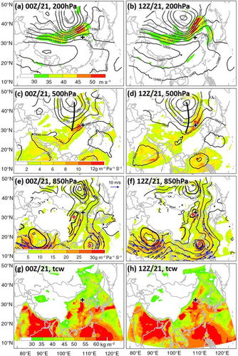
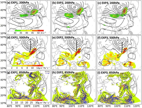
This heavy rainfall event occurred in an environment with a possible interaction among several synoptic weather systems. From 0000 UTC 21 July to 1200 UTC 21 July, an upper-level jet stream at 200 hPa intensified (Fig. 2a and b) to the north of Beijing (the location of Beijing is denoted by the black cross). At 500 hPa, a pronounced trough in the westerly flow extended southward from the centre of a quasi-stationary cold vortex in Mongolia and moved eastward, approaching the Beijing area (Fig. 2c and d). At 850 hPa, a low-pressure centre underneath the upper-level trough propagated towards the Beijing area from the southwest (Fig. 2e and f). With the intensification of the low-pressure centre, a low-level jet to the southeast of the low appeared and strengthened. In the meantime, Typhoon Vicente (2012) and a monsoon low were located, respectively, in the South China Sea and the Bay of Bengal. Moisture was transported to the Beijing area from the southwest at the middle level (Fig. 2c and d) in front of the trough and from the southwest and south originating from the South China Sea at a lower level (Fig. 2e and f). This moisture channel can be clearly seen from the distribution of the total column water (Fig. 2g and h). A large amount of moisture, 45 kg m⁻² D03-averaged total column water at 0000 UTC 21 July and 57 kg m⁻² at 1200 UTC 21 July, was transported northward and converged in the Beijing area.

Fig. 2 The ECMWF analyses at 0000 UTC 21 July 2012 (left panels) and 1200 UTC 21 July 2012 (right panels) of (a, b) 200-hPa wind speed (shaded, m s⁻¹) and geopotential height (contour, every 60 gpm), (c and d) 500-hPa geopotential height (contour, every 40 gpm) and horizontal water vapour flux (shaded, g m⁻¹ Pa⁻¹ s⁻¹) with the thick black line representing the trough axis, (e and f) 850-hPa geopotential height (black contour, every 20 gpm), wind vectors with a speed larger than 10 m s⁻¹ and horizontal water vapour flux (shaded, g m⁻¹ Pa⁻¹ s⁻¹), and (g and h) total column water (tcw) (shaded, kg m⁻²). The red cross in (e) and (f) represents the location of the low-pressure centre at 850 hPa. The red typhoon symbol represents the location of typhoon Vicente. The black cross in each panel represents the location of the Beijing metropolitan area.

3. Performance of the operational forecast guidance

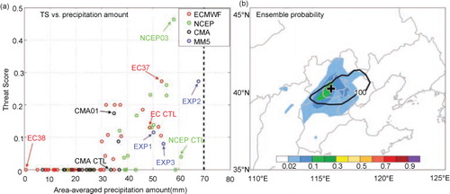
The ensemble and the control deterministic forecasts of the 24-h accumulated rainfall from 0000 UTC 21 July to 0000 UTC 22 July provided by ECMWF, NCEP and CMA (Fig. 3) showed a quite large uncertainty in terms of the pattern, location and amount, with an apparent underestimation of the peak magnitude of rainfall. Some members did realistically capture the distribution of the 24-h rainfall, while some members had quite large errors in either the pattern or location of the 24-h rainfall. To quantify the ensemble rainfall forecast skill for different scales, three areas (D01, D02 and D03 in Fig. 1) were used to calculate domain-averaged rainfall. The innermost D01 basically covers the area where the 24-h rainfall was larger than 300 mm. D02 generally covers the area where the 24-h rainfall was larger than 200 mm. D03 largely covers the area where the 24-h rainfall was larger than 100 mm. In the grand ensemble, about 9% of the ensemble members forecasted a D03-averaged precipitation amount larger than 50 mm, and about 9% of the ensemble members whose threat score (TS) calculated within the D03 at a threshold of 100-mm rainfall in 24 h (0000 UTC 21 July to 0000 UTC 22 July 2012) were larger than 0.2 (Fig. 4a). TS is defined as TS=H/(F+O−H) for precipitation above a certain threshold, where H is the number of points with correctly predicted precipitation, F is the number of points with predicted precipitation and O is the number of points with observed precipitation (Anthes et al., 1989). The ensemble probability of 100-mm precipitation showed that the maximum probability was less than 0.2, and the pattern of the probability was generally consistent with the observed precipitation (Fig. 4b), which suggests a quite large uncertainty in the ensemble rainfall forecasts.

Fig. 3 The distributions of 24-h rainfall control and ensemble forecasts from ECMWF, NCEP and CMA. Three good members (EC37, NCEP03 and CMA01) are marked by red boxes and one bad member (EC38) is marked by a blue box. The deterministic control forecasts of the three centres are marked by black boxes.

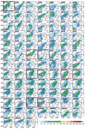
Fig. 4 (a) Domain-averaged rainfall vs. TS scatterplot. The TS was calculated within the D03 (shown in Fig. 1a) at a threshold of 100-mm rainfall in 24 h (0000 UTC 21 July to 0000 UTC 22 July 2012). The corresponding results of the control forecast from each centre and EXP1–3 are also plotted. The dashed black line represents the observed domain-averaged rainfall. (b) The observed (contour) and ensemble probability (shaded) of 100-mm 24-h rainfall. The black cross in (b) represents the location of the Beijing metropolitan area.

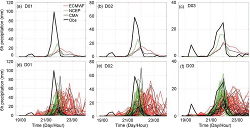
The evolution of the rainfall was also evaluated in terms of 6-h accumulated rainfall averaged over the three areas (D01, D02 and D03 in Fig. 1). The accumulation period for a certain time was the 6 h before the given time. The results showed that both the ensemble mean (upper panels of Fig. 5) and most of the individual members (lower panels of Fig. 5) underestimated the rainfall amount averaged over the three domains and with a time lag of 0–12 h. The magnitude and timing errors were the largest for the rainfall averaged over D01 (Fig. 5a and d) likely because of the low resolution. The maximum observed averaged rainfall was about 70–90 mm larger than the mean forecast. With the increasing of the average domain, the predicted rainfall came closer to the observations in terms of not only the rainfall amount but also the temporal distribution (Fig. 5a–c). The mean error decreased to 30–50 mm for D02. For the rainfall averaged over D03, the least magnitude and timing errors were observed. The rainfall magnitude error of the ensemble mean dropped to only about 10–15 mm. The timing error was about a 12-h delay for D01 and D02 and dropped to less than 6 h for D03. A large ensemble spread was observed in terms of the D03-averaged rainfall, with some members accurately capturing the observed rainfall. Consequently, the rainfall averaged over D03 was used for the sensitivity analyses to identify the key synoptic systems in Section 4.

Fig. 5 The evolution of 6-h domain-averaged rainfall forecast over D01 (a and d), D02 (b and e) and D03 (c and f) from the ensemble mean (a–c) and individual ensemble member (d–f) of ECMWF (red), NCEP (green) and CMA (black). The heavy black line in each panel denotes the corresponding observations.

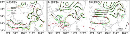
Different performances of the ensemble forecasts were observed among different NWP centres (Fig. 5). For the peak rainfall stage, the ensemble forecasts of NCEP were clearly more accurate than those of ECMWF and CMA in this particular case in terms of both the timing and peak value of the rainfall. There was a much larger uncertainty in the ECMWF and CMA ensemble forecasts than in the NCEP ensemble forecasts. The initial conditions from different centres were compared in terms of the geopotential height at 200, 500 and 850 hPa (Fig. 6). The main differences were mainly at 500 hPa around the Tibetan Plateau area and southern tip of the trough near (40°N, 95°E). The southern end of the trough of CMA was located to the west of those of NCEP and ECMWF. The significant difference near the Tibetan Plateau might have contributed to the significant difference in the forecast of the lower level low to the southwest of Beijing area. At the initial time, NCEP had the smallest ensemble spread in terms of the difference total energy, followed by ECMWF and CMA (figures not shown), which was consistent with the ensemble spread of different centres at the forecast time.

Fig. 6 The ensemble mean of the geopotential height from ECMWF (red), NCEP (green) and CMA (black) at 0000 UTC 18 July 2012 at (a) 850 hPa, (b) 500 hPa and (c) 200 hPa. The black cross in each panel represents the location of the Beijing metropolitan area.

4. Sensitivity analyses: ensemble-based correlation

4.1. The grand ensemble–based linear correlation coefficient

Linear correlation coefficients between the 24-h (0000 UTC 21 July–0000 UTC 22 July) domain-averaged rainfall and various variables at different times were calculated to explore the strength of a possible linear relationship. The linear correlation coefficient was calculated as follows:1

where x and y are two different variables, the overbar represents the mean of the variable, n represents the dimension of x and y, and cor is the correlation coefficient between x and y. For an ensemble with 84 members, the correlation coefficient with an absolute value of larger than 0.28 has a confidence level of 99% according to the two-tailed significance test (Fisher, 1925).

The correlations between the D03-averaged 24-h accumulated rainfall (0000 UTC 21 July–0000 UTC 22 July) and different variables at 1200 UTC 21 July are given in Fig. 7. The results showed that the rainfall was closely correlated with a jet stream at the 200-hPa level (Fig. 7a). Two positive correlation areas were identified: one was located along the ensemble mean jet stream and the other was located to the southwest of the jet stream. Two negative correlation areas were identified to the northwest and southeast of the jet stream. These results suggest that an upper-level jet that was located more to the east was associated with more forecast rainfall in the Beijing area.

Fig. 7 The correlation coefficient (shaded) between the D03-averaged 24-h rainfall (0000 UTC 21 July to 0000 UTC 22 July 2012) and (a) 200-hPa wind speed, (b) 500-hPa geopotential height and (c) 850-hPa geopotential height at 1200 UTC 21 July 2012. The contours in each panel denote the ensemble mean: (a) 200-hPa wind speed larger than 30 m s⁻¹ (every 10 m s⁻¹), (b) 500-hPa geopotential height (every 40 gpm) and (c) 850-hPa geopotential height (every 20 gpm). Also given are the forecasts of 200-hPa wind speed (shaded, m s⁻¹) and geopotential height (contour, every 60 gpm), 500-hPa geopotential height (contour, every 40 gpm) and horizontal water vapour flux (shaded, g m⁻¹ Pa⁻¹ s⁻¹), and 850-hPa geopotential height (contour, every 20 gpm), horizontal water vapour flux (shaded, g m⁻¹ Pa⁻¹ s⁻¹) and wind vectors with a speed larger than 10 ms⁻¹ at 1200 UTC 21 July 2012 of (d–f) EC37 (good) and (g–i) EC38 (bad). The black cross in each panel represents the location of the Beijing metropolitan area.

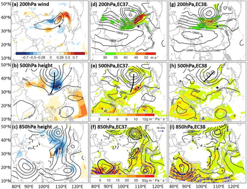
At 500 hPa, a dipole of positive and negative correlation patches straddled the trough in the westerly flow in the correlation field between the rainfall and geopotential height (Fig. 7b). The negative patch was over and slightly to the east of the trough with a larger area than that of the positive patch to the west of the trough. This suggests that a stronger and more easterly trough was associated with more rainfall in the Beijing area. Similar characteristics were also found at 700 hPa except that the trough shifted more to the east than that at 500 hPa (figures not shown).

At 850 hPa, there was one large negative patch extending southward from the cyclone centre at about 45°N with a stronger correlation in the southern part. This result suggests that a stronger cold vortex was associated with more rainfalls (Fig. 7c). The strong correlation centre actually corresponded to a low-pressure centre in some individual members, which will be detailed later. This result suggests that a stronger and more easterly low-pressure centre near (34°N, 110°E) was associated with more rainfalls.

The above instantaneous correlation analyses demonstrated that the dominant weather systems influencing the rainfall were the upper-level jet stream and the trough in the westerly flow as well as the low-level low-pressure system that developed under the trough considering their higher correlation coefficients. A large error in the intensity and locations of the above systems would lead to poor prediction of the rainfall. Comparing the maximum correlation coefficient at different levels (0.73 at 200 hPa, −0.76 at 500 hPa and −0.84 at 850 hPa), the most significant correlation was found at the low-pressure centre at 850 hPa, indicating that the most relevant system was likely the low at 850 hPa near the Beijing area.

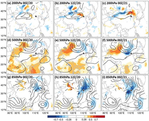
These highly correlated systems were further confirmed by analysing time-lag correlations between the domain-averaged 24-h rainfall from 0000 UTC 21 July to 0000 UTC 22 July and different variables at different forecast times before 1200 UTC 21 July (Fig. 8). These results showed that the high correlations became significant around 0000 UTC 20 July (Fig. 8a, d, g) about 48 h into the integration and 24 h before the beginning of the rainfall, and propagated with the upper-level jet stream, the cold vortex, the embedded trough in the westerly flow and the low-level low (Fig. 8).

Fig. 8 The correlation coefficient (shaded) between the D03-averaged 24-h rainfall (0000 UTC 21 July to 0000 UTC 22 July 2012) and (a–c) 200-hPa wind speed, (d–f) 500-hPa geopotential height and (g–i) 850-hPa geopotential height at (a, d, g) 0000 UTC 20 July, (b, e, h) 1200 UTC 20 July and (c, f, i) 0000 UTC 21 July 2012. The contours in each panel denote the ensemble mean: (a–c) 200-hPa wind speed larger than 30 m s⁻¹ (every 10 m s⁻¹), (d–f) 500-hPa geopotential height (every 40 gpm) and (g–i) 850-hPa geopotential height (every 20 gpm). The black cross in each panel represents the location of the Beijing metropolitan area.

4.2. Comparison between individual good and bad members

A good and a bad members were selected from the grand ensemble to exemplify the correlations obtained in the last section. EC37, with a high TS and a large amount of rainfall averaged over D03, was chosen as the good member, and EC38, with a low TS and little rainfall, was selected as the bad member (Figs. 3 and 4a).

Comparisons of the synoptic features between the good and bad members confirmed the high linear correlations between the rainfall and the upper-level jet stream, mid-level trough and low-level low. The intensity, location and morphology of these three environmental factors at 1200 UTC 21 July 2012 in the good member (Fig. 7d–f) were all closer to those in the analyses (Fig. 2b, d and f) than in the bad member (Fig. 7g–i). Relative to the bad member (EC38), the good member (EC37) produced a much stronger upper-level jet with a northeast-southwest orientation to the northeast of Beijing (Fig. 7d and g), a deeper mid-level trough that was located more to the east and thus transported more moisture to the Beijing area (Fig. 7e and h), and a stronger low-level cyclone to the north and a stronger low to the southwest of Beijing (Fig. 7f and i).

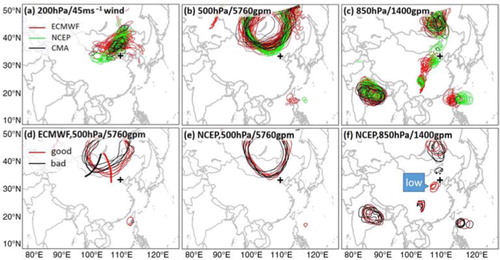
The importance of the low-level low-pressure centre can be seen more clearly when we compared the synoptic features of individual member. The spaghetti plots of the 45-m s⁻¹ wind speed at 200 hPa, 5760-gpm height at 500 hPa and 1400-gpm height at 850 hPa of the grand ensemble showed that the main differences were in the mid-level trough and the associated low-level low (Fig. 9a–c). The largest difference was in the forecast of the 1400 gpm (corresponding to the low-level low) to the southwest of the Beijing area (Fig. 9c). NCEP performed the best in this regard followed by ECMWF with the CMA having the worst forecast, which was consistent with their rainfall forecast skills. Much smaller differences were found in the 200-hPa jet, the tropical cyclone and the monsoon low. The significance of the 500-hPa trough was confirmed when we compared the best five and the worst five members in the ECMWF ensemble (Fig. 9d), which showed that the 500-hPa trough in the best members were located consistently more to the east and deeper. NCEP had the smallest error in 5760 gpm (corresponding to the mid-level trough) (Fig. 9b) among the three centres. Their 500-hPa trough was similar between the five best and the five worst members (Fig. 9e). What made the difference in the NCEP ensemble was the capability in capturing the low-level low-pressure system (Fig. 9f). This result indicates that the most important synoptic feature was likely the low-level low-pressure system, which is consistent with its higher correlation with the rainfall than other synoptic features.

Fig. 9 The forecasts of (a) 45 ms⁻¹ wind speed at 200 hPa, (b) 5760 gpm at 500 hPa and (c) 1400 gpm at 850 hPa at 1200 UTC 21 July from all ensemble members of ECMWF (red), NCEP (green) and CMA (black). Also shown are 5760 gpm at 500 hPa of the best five and worst five members from (d) ECMWF and (e) NCEP and (f) 1400 gpm at 850 hPa of the best five and worst five members from NCEP. The ‘low’ in (f) denotes the location of the low-level low-pressure system. The black cross in each panel represents the location of the Beijing metropolitan area.

4.3. Comparison between good members from ECMWF, NCEP and CMA

The best members from the three NWP centres (NCEP03, EC37 and CMA01, Table 1) were compared to further highlight the importance of the dominant features identified by the correlation analyses. Their TSs of the 24-h accumulated rainfall ranged from 0.17 to 0.46 in the order of CMA01, EC37 and NCEP03. The maximum 24-h accumulated rainfall of NCEP03 was 58.05 mm, about 5 mm higher than that of EC37 and about 24 mm higher than that of CMA01. The pattern of the 24-h accumulated rainfall (red boxed in Fig. 3) and the evolution of the 6-h domain-averaged rainfall of NCEP03 were both much closer to the observations than those of EC37 and CMA01 (Fig. 10).

Fig. 10 Same as Fig. 5f but only for the members of EC37, NCEP03 and CMA01 and the observation.

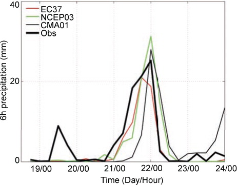
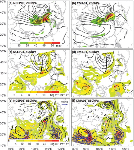
Table 1. The TS and magnitude of 24-h rainfall of good members from ECMWF, NCEP and CMA

	TS	Rainfall (mm)
NCEP03	0.46	58.05
EC37	0.27	53.34
CMA01	0.17	34.83

The results showed that the good performances of the three good members were likely due to similar reasons. They all captured the 200-hPa jet stream, 500-hPa trough and 850-hPa cyclone and low at 1200 UTC July 21 (Figs. 11 and 7d–f). Relative to EC37, NCEP03 and CMA01 produced a low-level low (Fig. 7f vs. Fig. 11e, f) more to the southwest, consistent with the locations of their accumulated rainfall (red boxed in Fig. 3). This result further confirmed the importance of the low-level low-pressure system to the rainfall.

Fig. 11 The forecasts from good members of NCEP03 (left panels) and CMA01 (right panels) at 1200 UTC July 2012, corresponding to forecast hour 84, of (a and b) 200-hPa wind speed (shaded, m s⁻¹) and geopotential height (contour, every 60 gpm), (c and d) 500-hPa geopotential height (contour, every 40 gpm) and horizontal water vapour flux (shaded, g m⁻¹ Pa⁻¹ s⁻¹) with the thick black line representing the trough axis, and (e and f) 850-hPa geopotential height (black contour, every 20 gpm), horizontal water vapour flux (shaded, g m⁻¹ Pa⁻¹ s⁻¹) and wind vectors with a speed larger than 10 m s⁻¹. The red cross in (e) and (f) represents the location of the low-pressure centre. The black cross in each panel represents the location of the Beijing metropolitan area.

4.4. Impact of the key synoptic features on the ingredients of heavy rainfall

The occurrence of heavy rainfall, especially convective heavy rainfall, has three ingredients: instability, moisture and lifting. It is interesting to know how the key synoptic features may have affected these ingredients in this case.

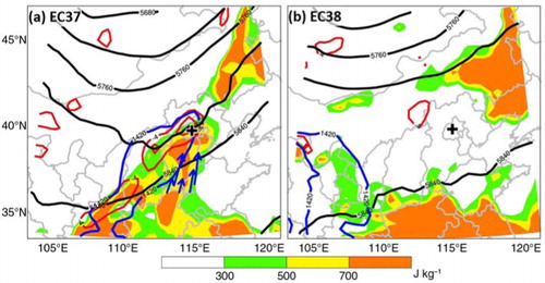
By examining situations in the good member (EC37), it was found that the 500-hPa trough and the associated low-level low-pressure centre had a significant impact on the three ingredients. First, the low-pressure centre at 850 hPa was well collocated with the maximum convergence (Fig. 12a), indicating a synoptic lifting. The southwesterly flow in front of the trough and the low-level jet associated with the low-pressure centre provided moisture to the rainfall region and converged there, which increased the instability, as indicated by the distribution of the convective available potential energy (CAPE). In the bad member (EC38), the trough was located far behind and much shallower than the observed one (Fig. 12b). No low-pressure centre was found near and to the southwest of the Beijing area. As a result, the moisture supply, synoptic lifting and instability were much weaker. The key role of the 500-hPa trough and its associated low-level pressure centre was further confirmed by the sensitivity analyses using the observation targeting strategy of CNOP, as shown in Section 5.

Fig. 12 The forecasts of CAPE (shaded, J kg⁻¹), geopotential height at 500 hPa (black contour, every 40 gpm), as well as 1420 gpm (blue contour), wind vectors with their speed larger than 12 m s⁻¹ and divergence at 850 hPa (red contour, s⁻¹) from (a) EC37 (the good member) and (b) EC38 (the bad member). The solid line represents divergence and the dashed line represents convergence. The black cross represents the location of the Beijing metropolitan area.

5. Sensitivity analyses: CNOP method

CNOP is the initial perturbation that maximises the forecast difference in terms of a given norm in the verification area at the verification time, which is the cost function J, between the nonlinear integrations initialised with and without the initial perturbation (Mu and Duan, 2003). The norm used to define J is the difference total dry energy (TDE′), which is calculated as follows:2

Thus the cost function is calculated as follows:3

where D denotes the horizontal verification area and η denotes the vertical coordinate. C_p is the specific heat at constant pressure (1005.7 J kg⁻¹ K⁻¹) and R_a is the gas constant of dry air (287.04 J kg⁻¹ K⁻¹). T_r (270 K) and P_r (1000 hPa) are the reference temperature and pressure. u′, v′, T′ and are the forecast differences of zonal and meridional wind components, temperature and surface pressure, respectively.

The adjustment of perturbations is made through an iteration method. For a given set of first-guess initial perturbations, the spectral projected gradient 2 (SPG2; Birgin et al., 2001) method is used to find further modified initial perturbations that make the cost function increase the most using the nonlinear model and the adjoint of the TLM. The iteration stops when the cost function converges to a maximum value. By using a set of first-guess initial perturbations, multiple final adjusted initial perturbations may be obtained. The final adjusted initial perturbations that produce the maximum cost function are defined as the CNOP. The area covered by the 1% of all points with the highest TDE′ of the CNOP is defined as the sensitive area that can be used to gather targeted observations.

The model used to produce the CNOP in this study was the fifth-generation Pennsylvania State University–National Centre for Atmospheric Research Mesoscale Model (MM5; Zou et al., 1997) and its tangent linear (TLM) and adjoint versions (ADM). A single domain (the outer domain of Fig. 13a) was used with a horizontal grid spacing of 60 km. The vertical coordinate had 21 levels with the top pressure level at 50 hPa. The initial and boundary conditions were provided by the NCEP FNL analysis data of 1°×1° at 6-h intervals. To obtain the evolution of the sensitive area, three experiments (denoted EXP1, EXP2 and EXP3) were performed using 0000 UTC 22 July 2012 as the verification time and 0000 UTC 20 July, 1200 UTC 20 July and 0000 UTC 21 July 2012 as the observation times, respectively. The verification area covered the location of the heavy precipitation (the inner box of Fig. 13a), which is similar to the domain used to produce the 24-h domain-averaged rainfall in the ensemble-based linear correlation analyses (D03 in Fig. 1).

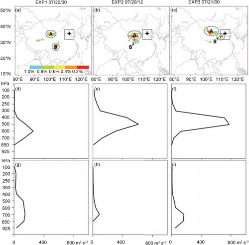
Fig. 13 The targeted area (TDE′, shaded) identified by the CNOP method for (a) EXP1, (b) EXP2 and (c) EXP3. The inner box in (a–c) denotes the verification area. The black cross in (a–c) represents the location of the Beijing metropolitan area. Also shown were the vertical distributions of the horizontal integrated TDE′ in the corresponding area A (d–f) and B (g–i).

The simulations of the 24-h rainfall (between 0000 UTC 21 July and 0000 UTC 22 July) initialised from the NCEP FNL analyses at different times in the three experiments (Fig. 14) were better than most members of the grand global forecast ensemble. Their TSs of the D03-averaged rainfall (0.115, 0.273 and 0.08 for EXP1, EXP2 and EXP3, respectively) were in the above 20th percentile of the grand ensemble (Fig. 4a). Their simulations of synoptic variables (Fig. 15) were also quite close to the global analyses (Fig. 2b, d and f). Consequently, the results of these experiments can be used to detect the sensitive area of the TDE′ in the verification area at the verification time.

Fig. 14 24-h accumulated rainfall (shaded, mm) from 000 UTC 21 July to 0000 UTC 22 July forecasted by (a) EXP1, (b) EXP2 and (c) EXP3. The inner box denotes the verification area.

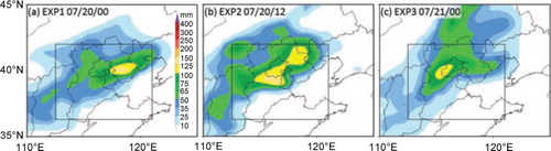
Fig. 15 The forecasts of EXP1 (left panels), EXP2 (middle panels) and EXP3 (right panels) at 1200 UTC July 2012 of (a and b) 200-hPa wind speed (shaded, m s⁻¹) and geopotential height (contour, every 60 gpm), (c and d) 500-hPa geopotential height (contour, every 40 gpm) and horizontal water vapour flux (shaded, g m⁻¹ Pa⁻¹ s⁻¹) with the thick black line representing the trough axis, and (e and f) 850-hPa geopotential height (black contour, every 20 gpm), horizontal water vapour flux (shaded, g m⁻¹ Pa⁻¹ s⁻¹), and wind vectors with a speed larger than 10 m s⁻¹. The red crosses in (g–i) represent the location of the low-pressure centre. The black cross in each panel represents the location of the Beijing metropolitan area.

In EXP3, which had the shortest lead time, two sensitive areas were identified by the CNOP (Fig. 13c). The vertical distribution of the horizontal integrated TDE′ (hTDE′) over area A peaked at 500 hPa (Fig. 13f), while the hTDE′ over area B peaked at 700 hPa (Fig. 13i). By overlapping the TDE′ with the geopotential height at 500 hPa, we can see that the sensitive area A was mainly located near the base of the mid-level trough (Fig. 16c), while the sensitive area B was mainly located near the low-level low (Fig. 16f). These results were quite consistent with the high correlation areas at the middle and lower levels obtained by correlation analyses.

Fig. 16 The targeted area (TDE′, shaded, m² s⁻²) identified by CNOP at (a) 600 hPa and (d) 700 hPa for EXP1, (b) 500 hPa and (e) 700 hPa for EXP2, and (c) 500 hPa and (f) 700 hPa for EXP3 and the geopotential height (contour, gpm) at the corresponding levels at their respective observation times. The thick black line represents the trough axis. The inner box in each panel denotes the verification area. The black cross represents the location of the Beijing metropolitan area.

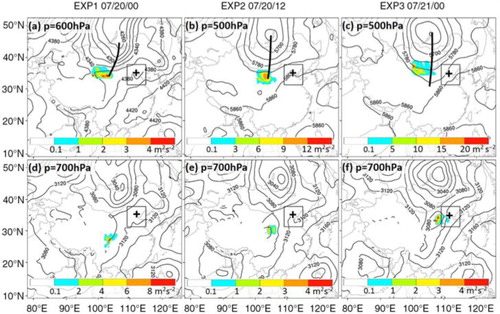
Experiments EXP2 and EXP1 with longer lead times, or earlier observation times, showed that the two sensitive areas clearly propagated with mid-level trough and the low-level low-pressure centre (Fig. 16). Their vertical distributions showed that the high sensitivities associated with the low-level low-pressure system generally stayed around 700 hPa (Fig. 13g–i), while the high sensitivities associated with the middle-level trough were located around a lower level of 600 hPa at earlier time and propagated upward to 500 hPa later on (Fig. 13d–f).

6. Summary and discussion

The high-impact heavy rainfall event in Beijing, China, on 21 July 2012 was investigated through ensemble-based linear correlation and CNOP methods to find the dominant synoptic weather systems influencing the heavy rainfall.

Large forecast uncertainties were observed in the location, pattern, magnitude and timing of the operational rainfall guidance. Although almost all the operational global NWP models severely underestimated the heavy rainfall of beyond 300 mm with ~12-h time lags, some of the ensemble members successfully captured the rainfall of beyond 100 mm at a scale of about 100 km with a time lag less than 6 h. Overall, NCEP ensemble forecasts produced more accurate rainfall forecasts than ECMWF and CMA for this case for various thresholds.

The grand ensemble forecasts of ECMWF, NCEP and CMA were used to perform the linear correlation analyses between the domain-averaged 24-h (0000 UTC 21 July–0000 UTC 22 July) accumulated rainfall over the area with the rainfall of beyond 100 mm and different variables at 1200 UTC 21 July. The results showed that the mid-level trough and the associated low-level low-pressure system were the most important factors associated with the heavy rainfall. In particular, a deeper mid-level trough in the westerly flow and stronger low-level low with a location closer to the Beijing area were associated with more rainfalls in Beijing. Relative to the mid-level trough, the low-level low pressure was more significantly correlated with the rainfall.

The dominant synoptic features identified by the ensemble-based linear correlation analyses, namely the 500-hPa trough and the associated low-level low, were further confirmed by the sensitive area identified using the CNOP observation targeting strategy. The sensitive area identified using a varying observation time propagated along with the trough and the low, which was consistent with the propagating features obtained using time-lag correlation analyses. The high sensitivities associated with low-level low pressure stayed generally around 700 hPa, while the high sensitivities associated with middle-level trough propagated from ~600 hPa to ~500 hPa during the 24 h before the rainfall event. Considering the results produced by the two sensitive methods, it was concluded that the low-level low was the most important weather system for the formation of this heavy rainfall event. This result also suggests that the CNOP method could be a good way to detect key precursors for high-impact weather systems.

These results of this work suggest that the major forecast errors for the 24-h accumulated 100-mm precipitation in this event might have mainly come from synoptic-scale features. Large uncertainties were found in the forecasted 500-hPa trough and associated low-level low in the grand ensemble. Further efforts will be made to explore the predictability of this high-impact event, such as the error growth dynamics as well as the sensitivities of the rainfall forecasts to model resolution and physical parameterisation schemes. However, considering that all the members underestimated the maximum rainfall even with a perfectly simulated synoptic feature, the extremeness in the rainfall of this event was likely determined by meso- or microscale systems that could not be resolved by current global models. A convection-allowing simulation is necessary to address the rainfall extremeness of this event.

7. Acknowledgements

This research was sponsored by the National Key Basic Research and Development Project of China under Grant 2013CB430104, and National Science Foundation of China Grants 41425018 and 41375048. Special thanks also go to the TIGGE data maintained by WMO.

References

- Anthes R. A. , Kuo Y.-H. , Hsie E.-Y. , Low-Nam S. , Bettge T. W . estimation of skill and uncertainty in regional numerical models. Q. J. R. Meteorol. Soc. 1989; 115: 763–806.
- Birgin E. G. , Martinez J. E. , Marcos R . Algorithm 813: SPG—Software for convex-constrained optimization. ACM Trans. Math. Softw. 2001; 27: 340–349.
- Bishop C. H. , Etherton B. J. , Majumdar S. J . Adaptive sampling with the ensemble transform Kalman filter. Part I: theoretical aspects. Mon. Weather Rev. 2001; 129: 420–436.
- Bougeault P. , Toth Z. , Bishop C. , Brown B. , Burridge D. , co-authors . The THORPEX interactive grand global ensemble. Bull. Am. Meteorol. Soc. 2010; 91: 1059–1072.
- Buizza R. , Hollingsworth A. , Lalaurette F. , Ghelli A . Probabilistic predictions of precipitation using the ECMWF Ensemble Prediction System. Weather Forecast. 1999; 14: 168–189.
- Chen B. Y . Observation system experiments for typhoon Nida (2004) using the CNOP method and DOTSTAR data. Atmos. Ocean. Sci. Lett. 2011; 4: 118–123.
- Chen Y. , Sun J. , Xu J. , Yang S. , Zong Z. , co-authors . Thinking on the extremes of the 21 July 2012 torrential rain in Beijing Part I: observation and thinking. Meteor. Monogr. 2012; 38(10): 1255–1266.
- Fisher R. A . Statistical methods for research workers. 1925; Edinburgh, UK: Oliver and Boyd. 378.
- Huang L. , Meng Z . Quality of the target area for metrics with different nonlinearities in a mesoscale convective system. Mon. Weather Rev. 2014; 142: 2379–2397.
- Lynch S. L. , Schumacher R. S . Ensemble-based analysis of the May 2010 extreme rainfall in Tennessee and Kentucky. Mon. Weather Rev. 2014; 142: 222–239.
- Mu M. , Duan W . A new approach to studying ENSO predictability: conditional nonlinear optimal perturbation. Chin. Sci. Bull. 2003; 48: 1045–1047.
- Mu M. , Zhou F. , Wang H . A method for identifying the sensitive areas in targeted observations for tropical cyclone prediction: conditional nonlinear optimal perturbation. Mon. Weather Rev. 2009; 137: 1623–1639.
- Mullen S. L. , Buizza R . Quantitative precipitation forecasts over the United States by the ECMWF Ensemble Prediction System. Mon. Weather Rev. 2001; 129: 638–663.
- Palmer T. N. , Gelaro R. , Barkmeijer J. , Buizza R . Singular vectors, metrics, and adaptive observations. J. Atmos. Sci. 1998; 55: 633–653.
- Qin X., Duan W., Mu M. Conditions under which CNOP sensitivity is valid for tropical cyclone adaptive observations. Q. J. R. Meteorol. Soc. 2013; 139: 1544–1554. DOI: http://dx.doi.org/10.1002/qj.2109.
- Qin X., Mu M. Influence of conditional nonlinear optimal perturbations sensitivity on typhoon track forecasts. Q. J. R. Meteorol. Soc. 2011; 138: 185–197. DOI: http://dx.doi.org/10.1002/qj.902.
- Reynolds C. A. , Rosmond T. E . Nonlinear growth of singular vector-based perturbations. Q. J. R. Meteorol. Soc. 2003; 129: 3059–3078.
- Schumacher R. S . Ensemble-based analysis of factors leading to the development of a multiday warm-season heavy rain event. Mon. Weather Rev. 2011; 139: 3016–3035.
- Schumacher R. S. , Davis C. A . ensemble-based forecast uncertainty analysis of diverse heavy rainfall events. Weather Forecast. 2010; 25: 1103–1122.
- Sippel J. A. , Zhang F . A probabilistic analysis of the dynamics and predictability of tropical cyclogenesis. J. Atmos. Sci. 2008; 65: 3440–3459.
- Sippel J. A. , Zhang F . Factors affecting the predictability of Hurricane Humberto (2007). J. Atmos. Sci. 2010; 67: 1759–1778.
- Sun J. , Chen Y. , Yang S. , Dai K. , Chen T. , co-authors . Analysis and thinking on the extremes of the 21 July 2012 torrential rain in Beijing Part II: preliminary causation analysis and thinking. Meteor. Monogr. 2012; 38(10): 1267–1277.
- Sun J. , Zhang X. , Wei J. , Zhao S . A study on severe heavy rainfall in north China during the 1990s. Clim. Env. Res. 2005; 10(3): 492–506.
- Xu J. , Chen Y. , Sun J. , Yang S. , Zong Z. , co-authors . Observation analysis of Beijing extreme flooding event 21 July 2012. Weather Forecast. Rev. 2012; 4(5): 9–19.
- Yu X . Investigation of Beijing extreme flooding event on 21 July 2012. Meteor. Monogr. 2012; 38(11): 1313–1329.
- Zhang D.-L., Lin Y., Zhao P., Yu X., Wang S., co-authors. The Beijing extreme rainfall of 21 July 2012: ‘Right results’ but for wrong reasons. Geophys. Res. Lett. 2013; 40: 1426–1431. DOI: http://dx.doi.org/10.1002/grl.50304.
- Zou X. L. , Vandenberghe F. , Pondeca M. , Kuo Y.-H . Introduction to adjoint techniques and the MM5 adjoint modeling system. 1997; Note, NCAR/ TN2435 + STR, Boulder, CO, USA: NCAR Technical. 110.