How northern freshwater input can stabilise thermohaline circulation

Abstract

The North Atlantic thermohaline circulation (THC) carries heat and salt towards the Arctic. This circulation is partly sustained by buoyancy loss and is generally believed to be inhibited by northern freshwater input as indicated by the ‘box-model’ of Stommel (1961). The inferred freshwater-sensitivity of the THC, however, varies considerably between studies, both quantitatively and qualitatively. The northernmost branch of the Atlantic THC, which forms a double estuarine circulation in the Arctic Mediterranean, is one example where both buoyancy loss and buoyancy gain facilitate circulation. We have built on Stommel's original concept to examine the freshwater-sensitivity of a double estuarine circulation. The net inflow into the double estuary is found to be more sensitive to a change in the distribution of freshwater than to a change in the total freshwater input. A double estuarine circulation is more stable than a single overturning, requiring a larger amount and more localised freshwater input into regions of buoyancy loss to induce a thermohaline ‘collapse’. For the Arctic Mediterranean, these findings imply that the Atlantic inflow may be relatively insensitive to increased freshwater input. Complementing Stommel's thermal and haline flow regimes, the double estuarine circulation allows for a third: the throughflow regime. In this regime, a THC with warm poleward surface flow can be sustained without production of dense water; a decrease in high-latitude dense water formation does therefore not necessarily affect regional surface conditions as strongly as generally thought.

• Box-model
• Arctic Mediterranean
• freshwater-sensitivity
• thermohaline circulation

1. Introduction

The Atlantic thermohaline circulation (THC) redistributes vast amounts of heat and salt (e.g. Kuhlbrodt et al., 2007). Heating of the ocean at low latitudes and cooling at high latitudes prescribes a poleward heat transport which is partly sustained by deep water formation in the North Atlantic Ocean and Nordic Seas, and upwelling in the south. The meridional gradient in surface heat fluxes induces a freshwater cycle with net evaporation from the warm waters and net precipitation and river runoff into the cold waters. This northern freshwater input is generally believed to inhibit the Atlantic THC as indicated by the box-model of Stommel (1961). We will argue, using an extension of this model, that this is not necessarily the case.

Stommel's box-model illustrates the influence of freshwater input on THC. The model consists of two well-mixed basins of water, one warm and one cold, which are connected along the surface and bottom to allow for an overturning circulation. The hydrostatic pressure difference at the bottom forces the deep cold water into the warm basin and induces a circulation; to compensate, warm water flows into the cold basin along the surface. In Section 2.3, we discuss to what extent this model can be projected on large-scale ocean circulation. Freshwater input into the model's cold basin inhibits this circulation and, when strong enough, induces a positive feedback between the volume transport and salt advection which leads to a reversal of the circulation. Hence, Stommel's model exhibits two stable circulation regimes.

Despite its idealised nature, or perhaps because of it, Stommel's model has provided much insight into the behaviour of THC. Although Stommel himself called it a ‘toy-model’ for the flow between two interconnected reservoirs, many analogies have been made with the Atlantic Meridional Overturning Circulation (AMOC). Bryan (1986) was the first to simulate multiple stable regimes of a THC in an ocean general circulation model (GCM), and Manabe and Stouffer (1988) found two stable regimes in a coupled ocean-atmosphere GCM. The analogy between Stommel's box-model and the Atlantic THC was further considered by Rahmstorf et al. (2005) who used the model to diagnose an AMOC ‘collapse’ in intermediate complexity GCMs in so-called freshwater hosing experiments. Such a collapse is often paralleled to a transition to a haline circulation regime, that is, a reversal. Recent GCM studies on the response of the AMOC to increased northern freshwater input over the 21st century, however, project a gradual weakening rather than a reversal, shutdown or even an abrupt reduction (Weaver et al., 2012).

The effect of salt advection on THC, as described by Stommel, is a direct result of the tendency of temperature to equilibrate faster than salt due to direct heat loss to the atmosphere. Another implication of this asymmetry between temperature and salinity is that combined heat loss and freshwater input can lead to initial buoyancy loss and subsequent buoyancy gain (Wåhlin et al., 2009). It is generally known that buoyancy gain can facilitate THC as well as buoyancy loss. In riverine outlets, freshwater input induces estuarine circulations due to entrainment of relatively saline surrounding water. Stigebrandt (1981) showed that also the upper circulation in the Arctic Ocean can be described as an estuarine circulation and it is the northern freshwater input that sustains this branch of THC. If we are to assess the influence of freshwater input on THC in general, it appears one needs to take into account both processes of buoyancy loss and buoyancy gain.

One example where both processes of buoyancy loss and buoyancy gain affect the circulation is the northernmost branch of the Atlantic THC. The Arctic Mediterranean forms an approximate semi-enclosed basin with the Greenland-Scotland Ridge (GSR) as its main gateway. The basin is subject to both heat loss and freshwater input which transforms an inflow of Atlantic water in two stages. First heat loss and freshwater input combine to induce net buoyancy loss, predominantly in the Nordic Seas and Barents Sea. Part of the produced dense water returns towards the Atlantic as overflow water (Isachsen et al., 2007): an overturning branch. The residual of the densified inflow is subject to net freshening and consequent buoyancy gain in the Arctic and eventually exits the Arctic Mediterranean as cold, fresh polar water through the East Greenland Current (Rudels, 1989): an estuarine branch. The combination of these overturning and estuarine branches comprises a double estuarine circulation (Stigebrandt, 1985; Rudels, 2010). Extending the classical model of Knudsen (1900) to a double estuary for the Arctic Mediterranean, Eldevik and Nilsen (2013) concluded that the present Atlantic inflow is more sensitive to changes in heat than freshwater fluxes.

Several authors have expanded Stommel's box-model to allow for more features of THC (Rooth, 1982; Welander, 1986; Thual and Mcwilliams, 1992; Rahmstorf, 1996). We will here construct a box-model which allows for THC associated with subsequent buoyancy loss and buoyancy gain. We do not aim for a fully realistic description of double estuarine circulation with all its processes and energetics. Rather, we aim to contrast the stability and freshwater-sensitivity of a double estuarine circulation to a single overturning circulation in an equivalent framework. In Section 2, we present two separate models for an overturning (Stommel, 1961) and an estuarine circulation (equivalent to Rooth, 1982); in Section 3, we construct a model for the double estuary and describe its qualitative behaviour. As a quantitative example, we will in Section 4 project the model onto the Arctic Mediterranean. Using this model, we show that a double estuarine circulation is more stable than a single overturning circulation. We further illustrate how a shutdown of dense water formation does not necessarily alter surface conditions qualitatively.

2. Overturning and estuarine circulation

Double estuarine circulation is the circulation of volume, heat and salt induced by two stages of watermass transformation due to surface buoyancy fluxes. A double estuary is the semi-enclosed basin in which the watermass transformation occurs. We will construct a minimal box-model for a double estuary subject to net heat loss and freshwater input which is in contact with an external reservoir of relatively warm, saline water (Fig. 1c). The three basins represent well-mixed reservoirs of the three associated watermasses, connected to allow two branches of circulation: an overturning and an estuarine branch.

Fig. 1 Three-box model configurations. (a) Overturning (negative estuarine) circulation with volume transport Ψ_O, identical to the configuration of Stommel (1961), (Section 2.1); F ₂ indicates the freshwater input into basin 2. (b) Estuarine circulation with volume transport Ψ_E, identical to the configuration of Rooth (1982), (Section 2.2). F ₂ and F ₃ indicate the freshwater input into the double estuary (basins 2 and 3). (c) Double estuarine circulation combining an overturning and estuarine branch (Section 3). The inflow transport Ψ_I into the double estuary is the sum of the overturning and estuarine transports. Arrows depict positive transports by convention.

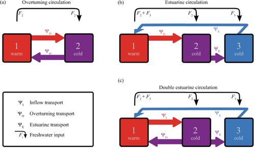
For the construction of his two-box model, Stommel (1961) argued that heat diffuses faster than salt. We will expand on this idea by allowing for watermass transformation to occur in two stages. In the first stage, both cooling and freshening occur on different time scales; in addition, a second stage allows for freshening without further cooling. This distinction allows for an inflow to initially lose buoyancy during the first stage and gain buoyancy during the second. Outflow of water produced in the first stage (basin 2) completes an overturning branch, whereas outflow of water produced in the second stage (basin 3) completes an estuarine branch.

In this section, we decompose the model into two separate circulations by allowing either of these outflows (Fig. 1a and b). These separated circulations are defined as an overturning and an estuarine circulation, respectively. The review of these models is in line with the overview of Marotzke (2000) and generally uses his nomenclature and dimensionalisations. We aim to understand how equilibrium volume transports and their stability depend on the freshwater input into the (double) estuary. For this, we apply linear stability analysis, described in Appendix A and identify different bifurcations (e.g. Kuznetsov, 2013) that characterise the qualitative stability of circulation.

2.1. Overturning circulation: Stommel (1961)

Overturning circulation only allows for outflow of the watermass produced in the first stage of transformation: cooling and freshening. For this circulation (Fig. 1a), we adopt Stommel's (1961) original box-model. This model consists of two well-mixed basins of water, connected by tubes of negligible volume. Conservation of salt in each of the basins can be written as1 2

where V _i is the volume of each basin; Ψ_O is the volume transport of the overturning, defined positive with surface flow from basin 1 to basin 2 (cf. Fig. 1a); ΔS _ij ≡ S _i – S _j is the salinity contrast between two basins; and F ₂ is the freshwater input into basin 2, parametrised as a virtual salinity flux. An equal freshwater flux out of basin 1 closes the total freshwater budget. We will constrain F ₂ to positive values.

Stommel closed the set of equations by assuming a linear relation between the volume transport and the hydrostatic pressure difference at the bottom of the basins. In order to contrast the double estuarine circulation to this well-established model for an overturning circulation, we generally assume the same linear relation introduced by Stommel. Further assuming a linear equation of state, we get a relation between the volume transport and the contrast in temperature and salinity between the basins:3

where ρ _i is the density in each basin; ρ _ref is a reference density; α and β are the thermal and haline expansion coefficients; ΔT is the temperature difference between the warm basin 1 and the cold basins 2 and 3; and k _O is a hydraulic constant, relating the overturning transport to the density contrast induced by the watermass transformation.

We assume temperatures to be constant, with ΔT>0. This assumption is equivalent to applying a restoring condition for temperature with immediate relaxation to an ambient value (Marotzke, 2000).

We non-dimensionalise the system by introducing:4 5 6

which implies a scaling for the volume transport:7

This scaling applies to all volume transports throughout this study. Inserting eq. (3) into eq. (1) and (2) gives a single non-dimensional dynamical equation for the salinity contrast between the basins:8

where the non-dimensional volume transport is:9

The equilibrium solutions, denoted throughout the paper with an asterisk *, of eq. (8) are:10

Note that these solutions are independent of the basin volumes. This is generally the case for all models presented in this study.

Combining eqns. (9) and (10) gives an equilibrium overturning transport as a function of the freshwater input into basin 2 (Fig. 2a). Each of the solutions in eq. (10) applies to a separate circulation regime. The first applies to the thermal regime (red curves in Fig. 2a), in which the surface transport is directed from basin 1 to basin 2 (cf. Fig. 1a). The negative root is stable and the positive root is unstable (cf. Appendix A.1). The second solution in eq. (10) applies to the haline regime (blue curve) in which the overturning is reversed with respect to the thermal regime.

Fig. 2 Bifurcation diagrams for Stommel and Rooth's models. (a) Equilibrium overturning transport as a function of freshwater input into basin 2. Red and blue curves indicate thermal and haline regimes, respectively. X's indicate saddle-node bifurcations [cf. eqns. (11) and (12)]. (b) Equilibrium estuarine transport as a function of freshwater input into basin 3. O indicates a Hopf bifurcation [cf. eqns. (22)]. In both panels, solid (dashed) lines indicate stable (unstable) equilibria.

Both stable thermal and haline equilibria are valid for a limited range of f ₂. The thresholds that limit these equilibria are characterised by saddle-node bifurcations as indicated by the X's in Fig. 2a and are given by11 12

where subscripts |_th and |_ha refer to the thermal and haline equilibria, respectively. Between these thresholds, a bistability region exists wherein both equilibria have a stable solution for the same amount of freshwater input.

The saddle-node bifurcations are a reflection of the salt-advection feedback in the system. Suppose that the system resides in its thermal equilibrium and f ₂=0. A slow increase in f ₂ will induce a salinity contrast and weaken the transport. Advection of salt by the inflow into basin 2 sustains the overturning circulation in its thermal regime. For values of , the weakening of the transport suppresses the salt advection sufficiently for the system to enter a positive feedback loop which deems the thermal equilibrium unstable. This leads to an abrupt transition to the haline regime, wherein the circulation is reversed (Ψ _O<0). To retrieve a thermal circulation, f ₂ must be decreased below , where the haline equilibrium is invalid. Note that this would require negative f ₂ implying net evaporation from basin 2.

Stommel's model thus illustrates how a thermally driven overturning circulation can be inhibited by freshwater input, and can reverse to a stable haline circulation when a certain threshold is crossed. In a double estuary, however, this is only one effect of freshwater input, since the second circulation branch is an estuarine branch, facilitated by freshwater input.

2.2. Estuarine circulation: Rooth (1982)

Equivalently to the overturning, we can extract the estuarine branch from the double estuarine circulation by allowing only outflow of the watermass produced in the second stage of watermass transformation (Fig. 1b). This model for an estuarine circulation consists of three basins, representing the three watermasses involved in the circulation. Warm, saline water from basin 1 is cooled and freshened as it flows into basin 2. Rather than a direct return flow as in the overturning circulation, this water undergoes subsequent freshening (buoyancy gain) as it flows into basin 3. The cold and fresh water from basin 3 then constitutes the outflow from the double estuary into basin 1. Closer inspection of this model reveals that the configuration is identical to the box-model of Rooth (1982), in his case representing a more global version of Stommel's model with one equatorial and two high-latitude basins. We will however restrict the application of this model to an estuarine circulation.

The second stage of watermass transformation induces a density difference between basins 2 and 3. We assume a linear relation between this density difference and the estuarine transport, equivalent to eq. (3). Further using the same formulation of salt conservation as for the overturning, we write the model equations as:13 14 15

with volume transport Ψ_E:16

Here, k _E is the hydraulic constant for the estuarine circulation. Two parameters now describe the freshwater forcing of the estuarine circulation. In eqns. (13–15), F ₂ represents the freshwater input during the first stage of watermass transformation, also associated with heat loss. F ₃ represents the subsequent freshwater input after all heat from the warm inflow is lost. These same parameters, F ₂ and F ₃, will force the double estuarine circulation presented in the next section.

It should be noted that eqns. (13–15) apply only to a counter-clockwise estuarine circulation (cf. Fig. 1b). Because the model is symmetrical, equations for the clockwise circulation can be found by simply interchanging basins 2 and 3. As we will show in the next section, a counter-clockwise circulation of the estuarine branch can always be sustained with positive freshwater input into basin 3 (F ₃>0) and we will therefore only consider Ψ_E>0.

By combining eqns. (13–15) and (16), and scaling the system according to eqns. (4–7), we derive:17 18

Here, is a non-dimensional parameter that sets the linear scaling of the estuarine circulation to density contrasts relative to that of the overturning circulation. For the estuarine circulation described in this section, this parameter is redundant, but it will become important for the double estuarine circulation. The non-dimensional volume transport of the estuarine circulation is:19

The equilibrium solutions for eqns. (17) and (18) are:20 21

The equilibrium transport is only dependent on the freshwater input into basin 3 (Scott et al., 1999). This relation can be recognised directly by inserting eq. (16) into eq. (15).

Although the equilibrium transport is independent on f ₂, this freshwater input does constrain the stability of the equilibrium. As shown in Appendix A.2, a Hopf bifurcation (O in Fig. 2b) appears when f ₃ drops below a certain value, dependent on f ₂. Since Hopf bifurcations are dependent on the transient response to a perturbation, and model timescales depend on basin volumes [eq. (4)], the location of the bifurcation is also dependent on the size of the basins:22

This value divides the equilibrium solution into a stable and an unstable region (Fig. 2b). For sufficient freshwater input into basin 3 , the estuarine circulation is stable, increases with f ₃ and is independent on f ₂. For , the positive circulation is unstable and the assumed positive estuarine circulation (Ψ_E>0) cannot be sustained. This instability is related to a positive feedback associated with the salt advection from basin 1 into basin 2 as discussed by Scott et al. (1999).

2.3. On model assumptions

The models for an overturning and estuarine circulation described above are essentially two configurations of the same model. Both configurations, as well as other varieties derived from Stommel's original concept, are by construction idealisations. This makes them analytically tractable and conceptually appealing. When constructing our double estuary model in Section 3, we will retain the model physics of Stommel (and Rooth). We can accordingly benefit from existing understanding and established concepts of THC (e.g. the salt-advection feedback) associated with these models, but we are at the same time adopting the assumptions and caveats of the model physics.

The main assumptions at the heart of the models presented in this study include: 1) constant temperatures; 2) a closed freshwater cycle; 3) well-mixed basins; and 4) volume transports scaling linearly with density differences between basins. The latter constitutes the model's dynamical closure that completes the mathematical formulation at the level of salt conservation. The schematic of ‘boxes and pipes’ (e.g. Fig. 1) is thus a visualisation of the salt budget and not concerned with the details of ocean circulation and ocean basins beyond salt conservation.

Temperature is generally understood to equilibrate faster than salinity. In the case of constant temperatures (equivalent to Marotzke, 2000), this equilibration takes place instantaneously compared to the time scale of the changing salt budget. In our specific application to the Arctic Mediterranean (Section 4), this time scale is equal to 40 yr when considering the typical temperature contrast between the North Atlantic and the Arctic Ocean (about 10 K, see Table 1). The simplest relaxation is to a constant temperature contrast. Although this is generally unrealistic, we may expect variations in temperature contrast between low and high latitudes on these temporal and spatial scales to be on the order of degrees, moderate compared to its mean.

Table 1. Model parameters

Parameter	Symbol	Value
Present state observations
Salinity contrast Atlantic inflow and overflows	ΔS 12	0.3 psu
Salinity contrast overflows and polar water	ΔS 23	0.9 psu
Temperature contrast Atlantic inflow and outflows	ΔT	8 K
Volume transport Atlantic inflow	ΨI	8.5 Sv
Volume transport overflows	ΨO	6 Sv
Parameters
Thermal expansion coefficient	α	10^−4 K^−1
Haline contraction coefficient	β	8×10^−4 psu^−1
Hydraulic constant overturning branch	k O	10^4 Sv
Hydraulic constant estuarine branch	k E	3×10^3 Sv
Volume basin 2	V 2	10^16 m^3
Scaling terms
Time	t	40 yr
Freshwater input (relative to 35 psu)	F i	230 mSv
Salinity contrast	ΔS ij	1 psu
Volume transport	Ψ	8 Sv

Thermohaline contrasts are from Eldevik and Nilsen (2013); volume transports from Hansen and Østerhus (2000).

In order to construct any model for THC which allows for non-transient equilibria, one requires a closed freshwater cycle or relaxation of salinity. The models presented here assume a closed freshwater cycle, where net evaporation instantaneously balances net freshwater input. This assumption appears less applicable in a regional setting, because salt is only conserved on a global scale. However, the sensitivity of salinity of each individual basin to the applied freshwater fluxes scales with the basin volumes. One can, for example, consider the limit of an arbitrarily large evaporating basin. In this limit, the evaporating basin retains a constant salinity and resembles a sponge layer, commonly applied in regional numerical simulations with GCMs. Freshwater parameters can then be interpreted as pure parameters of freshwater input. It is important to note here that equilibrium solutions of these models are generally independent on the choice of basin volumes.

The assumption of well-mixed basins invites for interpretation of these basins as reservoirs of certain water masses, by definition relatively homogeneous, rather than ocean basins. Advection of volume and salt between basins then requires transport through isopycnals dividing the associated water masses. By retaining volume in each basin, in other words restricting movement of these isopycnals, the models imply diapycnal mixing which is unspecified and excessive (e.g. Nilsson and Walin, 2001).

Also the assumption of linear scaling of volume transport with density differences is associated with excessive mixing. Guan and Huang (2008) showed that accounting for limited mixing energy can be expressed in a non-linear scaling in Stommel's model. This scaling reduces the sensitivity of circulation to changes in surface buoyancy fluxes, which should be taken into account when interpreting the quantitative analysis in Section 4.

The linear scaling of volume transport with density difference as introduced by Stommel has been a common and valid critique when applying the model to large-scale THC. The relation cannot be straightforwardly deduced from first principles (Marotzke, 2000). The simulated AMOC of many GCMs do however scale linearly with the meridional density or hydrostatic pressure gradient (e.g. Griesel and Maqueda, 2006). Whether this consistency also reflects causality is admittedly a matter of much debate (Toggweiler and Samuels, 1995; Kuhlbrodt et al., 2007; de Boer et al., 2010).

In the case of the estuarine circulation, and particularly that associated with the Arctic, a linear scaling has been proposed by Werenskiold (1935). This argument, later adopted by Rudels (2010), is based on thermal wind balance between a fresh western boundary current (the outflow of the estuarine circulation) and relatively saline surrounding water. To what extent this holds and, more generally, how large-scale (Arctic) estuarine circulation is forced are also matters of debate (e.g. Rudels, 2012).

3. Double estuary model

The double estuarine circulation (Fig. 1c) allows for outflow of both watermasses produced during the first (basin 2) and second (basin 3) stages of transformation. The total circulation thus constitutes two branches: an overturning and estuarine branch. These two branches connect through the surface flow between basin 1 and 2 which is the inflow into the double estuary, defined as Ψ_I.

3.1. Model configuration

The volume transports of the separate branches, Ψ_O and Ψ_E, scale to density differences as in Stommel's and Rooth's models [eqns. (3) and (16)]. Conservation of volume implies:23

Scaled according to eq. (7), this can be written as:24

Here, we see that κ introduces a relative weight of the two stages of watermass transformation.

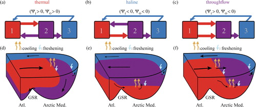
As discussed in Section 2.2, we will only consider Ψ _E=κ s ₂₃>0. Equation (24) then reveals three possible circulation regimes for the double estuarine circulation: the thermal, haline and throughflow regimes (Fig. 3a–c). The first two are qualitatively equivalent to the thermal and haline regimes of Stommel's overturning. The throughflow does not contain an overturning, neither thermal nor haline; rather, a flow is directed from basin 1 to basin 2 both at the surface and at depth.

Fig. 3 Three flow regimes of the double estuary. (a–c) Qualitative flow directions which define the different regimes. (d–f) An interpretation of the corresponding regimes in an Arctic Mediterranean setting. The present state of the Arctic Mediterranean can be characterised as a thermal circulation (panel d).

The equations for conservation of salt, applying to all three circulation regimes, can be written as:25 26 27

This is a generalisation of the equations for each separate regime, given explicitly in Appendix B. In terms of non-dimensional salinity contrasts, combining eqns. (24) and (25–27), we derive:28 29

3.2. Three stable regimes of flow

Both overturning and estuarine circulations showed that stability of circulation regimes can be constrained by certain values of freshwater input (cf. Section 2), and we may expect similar constraints to apply to the three regimes of the double estuarine circulation. We now pose the question for what range of freshwater parameters f ₂ and f ₃ the three circulation regimes have stable solutions. To answer this question, we again solve for the equilibrium solutions in terms of salinity contrasts s ₁₂ and s ₂₃, and determine the different bifurcations that limit the stability of the three regimes.

In eq. (27), we recognise the salt balance in basin 3 from Rooth's model [eq. (15)]. This reveals that we again have one equilibrium solution for s ₂₃,30

and consequently, the equilibrium transport of the estuarine branch, , is unaffected by the overturning branch [cf. eq. (19)]; it is still determined only by the freshwater input into basin 3. Hence, if there is no freshwater input into basin 3, there is no estuarine branch and the system is identical to Stommel's single overturning. This can be seen directly from eq. (28) with f ₃=0 and s ₂₃=0.

With Stommel's solution for a single overturning appearing as the limiting solution for f ₃=0, the question remains what solutions are possible with non-zero flow through the estuarine branch. The equilibrium solutions for s ₁₂ from eqns. (28) and (29) are:31

These three solutions apply to the thermal, haline and throughflow regimes, respectively (cf. Fig. 3a–c; with f ₃=0 being the equilibria of Stommel, eq. (10).

The stable regions for the three circulation regimes, derived from eqns. (30) and (31), are shown in a phase-space diagram as a function of f ₂ and f ₃ (Fig. 4). Some of the limits of these stable regions are determined by saddle-node bifurcations (solid lines in Fig. 4). Each equilibrium solution in eq. (31) has one saddle-node bifurcation; for the thermal regime, this forms an upper limit for the freshwater input f ₂ for which the circulation is stable; for the throughflow and haline regimes, it forms a lower limit. These saddle-node bifurcations can be expressed analytically as a function of f ₃ (see also Appendix A):32 33 34

Fig. 4 Phase-space diagram for the double estuarine circulation. Colour shading indicates which circulation regime(s) can be stable as a function of both freshwater parameters f ₂ and f ₃. So-called bistability occurs where two regimes overlap. Solid lines indicate saddle-node bifurcations [cf. eqns. (32–34)]; the dashed line indicates a Hopf bifurcation [eq. (22)]. The diagram is drawn for the symmetrical case κ=1 and V ₁=V ₂=V ₃.

Note that both equilibrium solutions and saddle-node bifurcations are independent on the basin volumes.

The only impact of basin volumes on the stability analysis of the double estuarine circulation comes from a Hopf bifurcation (dashed line in Fig. 4). This bifurcation limits the stability of the throughflow regime by the same constraint as for the estuarine circulation [eq. (22)]. Crossing these bifurcations leads to an abrupt transition from one circulation regime to another. Continuous transitions between neighbouring regimes, however, are also possible. We observe that the throughflow and haline regimes do not share a common bistability region and as a result transitions between these two regimes are always continuous.

The (in)stability of the thermal circulation in the double estuary is governed by the same salt-advection feedback as was present in Stommel's two-box model. The point where this feedback deems the circulation unstable is determined by [eq. (32)], which shifts to larger values of f ₂ when f ₃ increases (cf. red line in Fig. 4). For larger values of f ₃, more freshwater is available to facilitate the estuarine branch. This branch provides additional salt from basin 1 into basin 2 and damps the salt-advection feedback. This delays a possible abrupt transition and allows for a thermal circulation to be sustained for larger values of freshwater input into basin 2 compared to the single overturning. The estuarine branch thus stabilises the thermal circulation.

4. Application to the Arctic Mediterranean

The Arctic Mediterranean – the Nordic Seas and Arctic Ocean combined – is perhaps the best known example of a large-scale double estuary. The exchanges across its main gateway, the GSR, are carried by three watermasses reflecting a double watermass transformation due to cooling and freshening. The initial transformation of Atlantic water induces buoyancy loss and production of dense water returning to the Atlantic as overflow water (Isachsen et al., 2007). The secondary transformation, occurring in the Arctic, is one of net buoyancy gain, producing low salinity water returning to the Atlantic as polar water (Rudels, 1989). The former loop is relatively dominant today, carrying about two-third of the circulation (cf. Table 1). The net water mass exchange at the GSR is thus associated with a relative dominance of heat loss and consequent buoyancy loss, and can therefore be characterised as a double estuarine circulation residing in its thermal regime. An illustration of thermal, haline and throughflow regimes in an Arctic Mediterranean setting is given in Fig. 3d–f.

Freshwater input into the Arctic Mediterranean is projected to increase over the 21st century (Rawlins et al., 2010), which makes this a region of interest with respect to changed surface buoyancy forcing. The qualitative analysis of our double estuary model in Section 3 revealed that an estuary branch can stabilise a thermally direct overturning. Using the Arctic Mediterranean as a specific example, we will illustrate the possible quantitative effect of this stabilisation.

We first interpret the model variables and parameters in the context of the Arctic Mediterranean and use observations to dimensionalise the model. We then place the present state of the circulation in the phase-space diagram (Fig. 4), and accordingly estimate the quantitative freshwater-sensitivity of a double estuarine circulation as illustrated by three hypothetical scenarios for increased freshwater input.

4.1. Interpretation of the model

The three basins of the box-model (Fig. 1c) are interpreted as reservoirs of the associated watermasses, as discussed in Section 2.3. Basin 1 then represents the above-thermocline North Atlantic, constituting warm, saline water; basin 2 represents the dense waters in the Nordic Seas; and basin 3 represents the reservoir of light polar water in the above-halocline Arctic Ocean and East Greenland Current.

For the volume exchange in and out of the Arctic Mediterranean, we neglect any volume fluxes associated with the Pacific inflow through the Bering Strait and with precipitation and river runoff. Both can be parametrised as contributions to freshwater input. Consequently, the only inflow of volume into the double estuary is that of warm saline Atlantic water, which will be interpreted as Ψ_I. The fraction of dense water produced in the Nordic Seas and Barents Sea that returns to the Atlantic as overflow water will be interpreted as Ψ_O. The residual densified inflow entrains into the polar water in the Arctic Ocean and ultimately exits through the East Greenland Current and Canadian Arctic Archipelago. The combined volume transport of this buoyant return flow to the Atlantic will be interpreted as Ψ_E. In order to redraw Fig. 4 for the double estuary of the Arctic Mediterranean, we need to estimate the relative basin volumes as well as κ.

The relative basin volumes determine the location of the Hopf bifurcation, limiting stability of the throughflow regime [eq. (22)]. Because the Arctic Mediterranean is a regional setting, we take V ₁ V _2,3, where the evaporating basin is arbitrarily large with respect to the Arctic Mediterranean. As discussed in Section 2.3, this limit makes the salinity of the Atlantic inflow independent on the freshwater input into the Arctic Mediterranean. Because Arctic polar water is confined by the halocline, whereas dense waters in the Nordic Seas extend to full depth through deep convection, we further take V ₂(entity)V ₃. In these limits, , indicating that the throughflow regime is unrestricted by the Hopf bifurcation.

Parameter κ determines the locations of the saddle-node bifurcations [eqns. (32–34)]. Inserting observed density contrasts and volume transports (Tab. 1; Hansen and Østerhus, 2000; Eldevik and Nilsen, 2013) into eqns. (3) and (16), we find κ=0.32. The scaling of the estuarine transport to density differences is thus a factor three smaller than that of the overturning transport. If these transports are related to the hydrostatic pressure difference across isopycnals dividing the associated watermasses, k _O should scale with the depth of the thermocline above the GSR (about 600 m), and k _E should scale with the depth of the Arctic halocline (about 200 m). We see that this difference in isopycnal depth can largely account for the value of κ, deduced from observations.

4.2. A relatively insensitive Atlantic inflow

Scaling the complete system by these observations according to eqns. (4–6), we redraw the phase-space diagram for the double estuary of the Arctic Mediterranean (Fig. 5a). This diagram maps out the qualitative regions where the three circulation regimes have stable solutions. Using this diagram, we will determine the position of the ‘present state’ of the Arctic Mediterranean and quantify the required freshwater perturbation to induce an abrupt transition.

The present state of the double estuarine circulation is defined as the unique point in phase space where both and are equal to observed transports (cf. Fig. 5b). Equivalently, the present state in Stommel's model is defined where is equal to observed transport and is zero. The latter is naturally aligned with zero polar freshwater input.

Fig. 5 Phase-space diagram for the Arctic Mediterranean. (a) As in Fig. 4, scaled as described in Section 4. (b) Stable region of the thermal regime. Contours, interval 1 Sv, indicate constant overturning (black) and estuarine transport (grey). Thick lines correspond to observed transports (cf. Table 1). Markers indicate the ‘present state’ in the double estuary model and in Stommel's model. (c) From the ‘present state’, three dashed lines indicate scenarios for increased freshwater input in the double estuary model. Arrows indicate the required freshwater increase along each scenario to induce an abrupt transition into either the throughflow or haline regime. An additional scenario is indicated for Stommel's model for increased Nordic freshwater input.

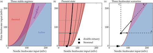
Starting with the present state forcing (cf. Fig. 5c), we assess the following hypothetical scenarios for increased freshwater input into the double estuary:

A: only Nordic freshwater input increases.

B: all freshwater input increases proportionally.

C: only polar freshwater input increases.

Each of these scenarios is projected as dashed lines in Fig. 5c. Along each line, we determine the value of as a function of the varying freshwater input and draw a bifurcation diagram for the Atlantic inflow (Fig. 6).

Fig. 6 Bifurcation diagram for three scenarios of increased freshwater input into the Arctic Mediterranean. Equilibrium solutions for Ψ_I ^* are shown along the trajectories A, B and C indicated in Fig. 5c. As a reference, the bifurcation diagram of the overturning (Stommel, Fig. 2a) is shown in the left panel. ‘Present state’ (triangle and square) is defined in Fig. 5b. Arrows are equivalent to those in Fig. 5b, indicating the required freshwater increase to destabilise the thermal circulation and induce an abrupt transition. The three Scenarios A, B and C are described in detail in the text.

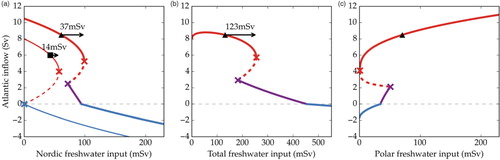
In Scenario A (Fig. 6a), the increase in freshwater input always weakens the Atlantic inflow since all additional freshwater enters in the stage of buoyancy loss, limiting the transport of the overturning branch while leaving the estuarine branch constant. An increase in Nordic freshwater input of 37 mSv destabilises the thermal circulation and induces an abrupt transition to the haline regime (see also Fig. 5c). Neglecting the estuarine branch and collapsing the system to a single overturning circulation (Stommel's model), an increase in Nordic freshwater input of 14 mSv is sufficient to induce a transition to the haline regime. In the double estuary model, the estuary branch advects additional salt to the regions of dense water formation, delaying a possible abrupt transition.

In Scenario B (Fig. 6b), increased freshwater input partly weakens the overturning branch and partly strengthens the estuarine branch. Because the weakening of the overturning appears dominant in this scenario, an increase in the total freshwater input inhibits the net Atlantic inflow and can destabilise the thermal circulation. Compared to Scenario A, this requires a larger increase in the total freshwater input (123 mSv) because of the stabilising salt advection through the estuarine branch. If an abrupt transition occurs under Scenario B, the circulation transits into the throughflow regime (see also Fig. 5c). During such a transition a warm Atlantic inflow persists and the surface conditions of the Arctic Mediterranean remain qualitatively the same (compare Fig. 3d and f).

Finally in Scenario C (Fig. 6c), increased polar freshwater input merely strengthens the estuarine branch. The associated salt transport from the Atlantic even facilitates dense water formation and increases the transport of the overturning branch slightly (not shown). Together, this leads to a strengthening of the Atlantic inflow and no abrupt transitions can occur.

Scenario B illustrates a possible transition from a thermal to a throughflow regime (cf. Fig. 3d and f). In the latter regime, the Atlantic inflow which carries salt towards the Arctic Mediterranean to balance net freshwater input is both along the surface and at depth. A necessary condition for this circulation to be realisable is that this inflow originates from warmer waters. Although this is likely because of its origin in lower latitudes, the quantitative temperature contrast beyond a transition to the throughflow regime cannot be estimated from this model. Rather, it needs to be determined a priori and for the illustration of Fig. 6, the temperature contrast is kept equal for all circulation regimes.

With these three scenarios, we illustrate a wide variety of possibilities for how freshwater input can affect THC. The most important factor in determining the circulation's response is the distribution of additional freshwater input. Estimates of projected increase in freshwater input in the Arctic Mediterranean primarily point to the increase in river runoff into the Arctic Ocean (Rawlins et al., 2010). We may therefore imagine a scenario between B and C as most appropriate for discussing quantitative change of the Arctic Mediterranean's THC.

In between these scenarios, Atlantic inflow is relatively insensitive to increased freshwater input. Estimates of long-term trends in Arctic sea ice melt are on the order of 10 mSv (500 km³/yr; Laxon et al., 2013). Whereas Stommel's model is very sensitive to a freshwater perturbation of this magnitude, it only impacts the double estuarine circulation significantly if all additional freshwater were to reach the Nordic Seas (cf. Fig. 6a). Rather than a significant change in the Atlantic inflow, the double estuary model shows a shift towards a more estuarine-dominated circulation where increased freshwater input weakens the overturning branch and strengthens the estuarine branch. A predominant role for freshwater in the branching of the circulation, rather than in restricting its total strength – the inflow – is also inferred from the diagnostics of Eldevik and Nilsen (2013).

5. Concluding remarks

GCMs used to quantify freshwater-induced changes in Atlantic THC in the framework of Stommel's box-model appear very sensitive to changes in northern freshwater input. Rahmstorf (1996) predicted a shutdown of the circulation when northern freshwater input is increased by 70 mSv. This value is comparable to the estimated increase in freshwater input into the Arctic and sub-Arctic seas over the 21st century, based on observations and model experiments (Rawlins et al., 2010).

Coupled atmosphere–ocean GCMs, projecting CO₂-induced changes in climate over this same period, however do not show a consistent sensitivity of the Atlantic THC to freshwater as opposed to heat (Gregory et al., 2005; Weaver et al., 2012). Specifically the northernmost branch of the THC in the Arctic Mediterranean appears less sensitive to freshwater than heat (Eldevik and Nilsen, 2013). By adding freshwater input in the order of 1.0 Sv into the North Atlantic in coupled GCMs, Stouffer et al. (2006) showed that deliberate water-hosing experiments are required to completely shut down the Atlantic overturning circulation. Our extension of Stommel's model into a double estuary illustrates how THC can be inherently more stable than a single overturning circulation.

The freshwater-sensitivity of a double estuarine circulation is qualitatively associated with the northern distribution of freshwater input. This distribution largely determines how additional total freshwater input may affect THC. In a limiting, most sensitive case where all freshwater feeds into the domain of dense water formation, the model is identical to that of Stommel (1961, Fig. 1a). The distribution of freshwater is directly linked to the pathways out of the double estuary, for example, in the case of the Arctic Mediterranean where much freshwater is exported via the East Greenland Current. Representation of the different watermass transformations and advective pathways additional to that of a single overturning circulation therefore appears essential for the freshwater-sensitivity of THC.

Our model for a double estuary accounts for a circulation branch that is sustained by buoyancy gain due to northern freshwater input: an estuarine branch, much like the Arctic estuarine circulation (Stigebrandt, 1981). This additional circulation branch damps Stommel's positive salt-advection feedback by providing a background salt import into the domain of dense water formation and hereby stabilises the overturning branch. A similar stabilisation was found when adding diffusion to Stommel's model to parametrise a wind-driven gyre (Longworth et al., 2005), and also Guan and Huang (2008); Nilsson and Walin (2001) concluded that THC is less sensitive to freshwater perturbations than Stommel's model when accounting for limited diapycnal mixing. These studies, including our study of a double estuary, all point in the same direction of a relatively weak freshwater-sensitivity of THC compared to that inferred from Stommel's model.

In the double estuary model, a proportional increase in northern freshwater input of 123 mSv is required to destabilise the overturning when an estuarine branch is accounted for (Fig. 6b). This value is an order of magnitude larger than the additional freshwater input required to destabilise the single overturning circulation of Stommel's model when scaled to the Arctic Mediterranean (Fig. 6a). Overall, a larger amount of freshwater feeding the estuarine branch allows the circulation to retain its qualitative state under larger increase in freshwater into the domain of dense water formation. For a certain range of distributions, additional northern freshwater input can even strengthen the THC (Fig. 6c). Because the overturning branch of the Arctic Mediterranean, including entrainment of Atlantic water into the overflows south of the GSR, is estimated to account for approximately 2/3 of the total AMOC (Dickson and Brown, 1994; Medhaug et al., 2012), stability of this northernmost branch of the Atlantic THC is important for sustaining a stable global overturning circulation (e.g. Jungclaus et al., 2006).

Abrupt reduction in THC is commonly associated with a cessation in open ocean convection (e.g. Dokken and Jansen, 1999). However, it is now understood that poleward heat transport and consequent northern heat loss are more directly related to ocean advection than convective mixing (Mauritzen, 1996; Fanning and Weaver, 1997; Pickart and Spall, 2007). Our model for the double estuary accommodates a third stable circulation regime, complementing the thermal and haline regimes introduced by Stommel. In this throughflow regime, the estuarine circulation dominates to the extent that net Atlantic inflow persists even in the case of absent or reversed overflow. This implies, at least in our model, that inflow can be sustained without dense water formation. More generally, we propose that an estuarine circulation extends the stability of poleward heat transport with respect to freshwater perturbations beyond the thermal regime.

6. Acknowledgements

This research was supported by the Centre for Climate Dynamics at the Bjerknes Centre for Climate Research through the Research Council of Norway project NORTH. Publication was funded by the University of Bergen. We thank Aleksi Nummelin, Lisbeth Håvik and two anonymous reviewers for their valuable input that improved the manuscript.

7. Appendix

A. Linear stability analysis

In order to determine whether a circulation can reside in a certain equilibrium state, we perform linear stability analysis on each equilibrium solution. This theory is based on linearisation of the model equations around a certain equilibrium and determining the growth rate of a perturbation. If this growth rate is negative, perturbations are damped and the equilibrium solution is stable; if the growth rate is positive, perturbations are amplified and the equilibrium is unstable.

Linearisation around an equilibrium is done by determining the Jacobian J. If the model consists of a single dynamical equation [as Stommel's model, cf. eq. (8)], this Jacobian is defined as:A1

and the equilibrium is stable if J<0. At the boundary between a stable and an unstable equilibrium, where J=0, a saddle-node bifurcation exists.

If the model consists of a system of two dynamical equations [as is the case for Rooth's model and our double estuary model, cf. eqns. (17), (18), (28) and (29)], the Jacobian is defined as:A2

In this case, two conditions determine a stable solution: det(J)>0 and trace(J)<0. The boundary det(J)=0 determines the location of a saddle-node bifurcation; trace(J)=0 determines the location of a Hopf bifurcation. Since we are merely interested in the stability of an equilibrium, we do not distinguish between stable nodes and foci.

A.1. Overturning circulation (Section 2.1)

Inserting eq. (8) into eq. (A1), we find for Stommel's overturning circulation:A3

As shown by Stommel (1961), for the thermal overturning (s ₁₂≤1), the negative root of eq. (10) is always stable and the positive root is unstable. The haline overturning (s ₁₂>1) is always stable. The points where stable and unstable equilibria meet are characterised by saddle-node bifurcations [eqns. (11) and (12)] as indicated in Fig. 2a.

A.2. Estuarine circulation (Section 2.2)

Inserting eqns. (17) and (18) into eq. (A2), we find for Rooth's estuarine circulation:A4

withA5 A6

Since det(J)>0 for all f ₃>0, no saddle-node bifurcations limit the stability of the estuarine circulation. However, a Hopf bifurcation appears at trace(J)=0, introducing a stability condition (cf. Scott et al., 1999),A7

which divides between a stable and an unstable equilibrium [eq. (22)] as indicated in Fig. 2b.

A.3. Double estuarine circulation (Section 3)

For the double estuary model, it is most convenient to perform linear stability analysis on each circulation regime separately.

A.3.1. Thermal regime (s ₁₂ ≤ 1)

For the thermal regime, the Jacobian is:A8

withA9 A10

As for the single overturning, a saddle-node bifurcation (det(J)=0) appears, deeming the negative root of eq. (31) stable and the positive root unstable. This saddle-node bifurcation is expressed in terms of f ₂ in eq. (11).

A Hopf bifurcation appears if trace(J)=0 and det(J)>0. This is possible ifA11

If f ₂ increases, this Hopf bifurcation destabilises the thermal regime before the saddle-node bifurcation can be reached.

In the symmetrical case of κ=1 and V ₁=V ₂=V ₃ (cf. Fig. 4), a Hopf bifurcation appears if . It can be shown that the maximum distance from the saddle-node bifurcation is 0.01 (in the case of f ₃=0). This means that the thermal regime becomes unstable at f ₂=0.24, rather than 0.25 as deduced from the saddle-node bifurcation. This effect is marginal, and no Hopf bifurcation can appear in the case of the Arctic Mediterranean where we take V ₂(entity)V ₃. We therefore do not pursue this possible instability further.

A.3.2. Haline regime (s ₁₂ >1+κs ₂₃ )

For the haline regime, the Jacobian is:A12

withA13 A14

Inserting eq. (31), we find that det(J)>0, trace(J)<0 for all values of f ₂, f ₃>0 and consequently the haline equilibrium always stable.

At the boundary between the haline and throughflow regimes, at s ₁₂=1+κs ₂₃, a saddle-node bifurcation appears if the throughflow equilibrium is unstable, as expressed in eq. (29). If the throughflow equilibrium is stable, there is no saddle-node bifurcation for the haline regime and transitions between the haline and throughflow regimes are smooth.

A.3.3. Throughflow regime (1 <s ₁₂ ≤ 1+κs ₂₃ )

For the throughflow regime, the Jacobian is:A15

withA16 A17

det(J) always positive, so a saddle-node bifurcation occurs where the throughflow regime meets the unstable branch of the thermal equilibrium at s ₁₂=1, as expressed in eq. (34).

Because the dynamics and consequently the equilibrium solutions of the throughflow regime are identical to those of the estuarine circulation of Rooth, a Hopf bifurcation appears at the same point: trace(J)=0 if , dividing a stable and an unstable throughflow circulation.

B. Salt conservation

Salt conservation in the double estuary model is expressed in single equations for each basin, general for each circulation regime [eqns. (25–27)]. Here, we provide the equations applied to each separate regime, dependent on the transport signs as indicated in Fig. 3a–c.

B.1. Thermal regime (Ψ _I>0, Ψ _O>0)B1 B2 B3

B.2. Haline regime (Ψ _I<0, Ψ _O<0)B4 B5 B6

B.3. Throughflow regime (Ψ _I>0, Ψ _O<0)B7 B8 B9

References

- Bryan F . High-latitude salinity effects and interhemispheric thermohaline circulations. Nature. 1986; 323: 301–304.
- de Boer A. M. , Gnanadesikan A. , Edwards N. R. , Watson A. J . Meridional density gradients do not control the Atlantic overturning circulation. J. Phys. Oceanogr. 2010; 40(2): 368–380.
- Dickson R. R. , Brown J . The production of North Atlantic Deep Water: sources, rates, and pathways. J. Geophys. Res. 1994; 99(C6): 12319–12341.
- Dokken T. M. , Jansen E . Rapid changes in the mechanism of ocean convection during the last glacial period. Nature. 1999; 401(6752): 458–461.
- Eldevik T. , Nilsen J. E. Ø. The Arctic–Atlantic thermohaline circulation. J. Clim. 2013; 26(21): 8698–8705.
- Fanning A. F. , Weaver A. J . A horizontal resolution and parameter sensitivity study of heat transport in an idealized coupled climate model. J. Clim. 1997; 10(10): 2469–2478.
- Gregory J. M. , Dixon K. W. , Stouffer R. J. , Weaver A. J. , Driesschaert E. , co-authors . A model intercomparison of changes in the Atlantic thermohaline circulation in response to increasing atmospheric CO2 concentration. Geophys. Res. Lett. 2005; 32(12): L12703.
- Griesel A. , Maqueda M. A. M . The relation of meridional pressure gradients to north Atlantic deep water volume transport in an ocean general circulation model. Clim. Dynam. 2006; 26(7–8): 781–799.
- Guan Y. P. , Huang R. X . Stommel's box model of thermohaline circulation revisited—the role of mechanical energy supporting mixing and the wind-driven gyration. J. Phys. Oceanogr. 2008; 38(4): 909–917.
- Hansen B. , Østerhus S . North Atlantic-Nordic seas exchanges. Prog. Oceanogr. 2000; 45(2): 109–208.
- Isachsen P. E. , Mauritzen C. , Svendsen H . Dense water formation in the Nordic seas diagnosed from sea surface buoyancy fluxes. Deep Sea Res. Part I Oceanogr. Res. Pap. 2007; 54(1): 22–41.
- Jungclaus J. H. , Haak H. , Esch M. , Roeckner E. , Marotzke J . Will Greenland melting halt the thermohaline circulation?. Geophys. Res. Lett. 2006; 33(17): 1–5.
- Knudsen M . Ein hydrographischer lehrsatz. Ann. Hydrogr. Marit. Meteorol. 1900; 28(7): 316–320.
- Kuhlbrodt T. , Griesel A. , Montoya M. , Levermann A. , Hofmann M. , co-authors . On the driving processes of the Atlantic meridional overturning circulation. Rev. Geophys. 2007; 45(2004): 1–32.
- Kuznetsov Y. A . Elements of Applied Bifurcation Theory, Vol. 112 . 2013; Springer Science & Business Media, New York.
- Laxon S. W. , Giles K. A. , Ridout A. L. , Wingham D. J. , Willatt R. , co-authors . Cryosat-2 estimates of arctic sea ice thickness and volume. Geophys. Res. Lett. 2013; 40(4): 732–737.
- Longworth H. , Marotzke J. , Stocker T. F . Ocean gyres and abrupt change in the thermohaline circulation: a conceptual analysis. J. Clim. 2005; 18(13): 2403–2416.
- Manabe S. , Stouffer R . Two stable equilibria of a coupled ocean-atmosphere model. J. Clim. 1988; 1(9): 841–866.
- Marotzke J . Abrupt climate change and thermohaline circulation: mechanisms and predictability. Proc. Natl. Acad. Sci. USA. 2000; 97(4): 1347–1350.
- Mauritzen C . Production of dense overflow waters feeding the North Atlantic across the Greenland-Scotland Ridge. Part 2: an inverse model. Deep Sea Res. Part I Oceanogr. Res. Pap. 1996; 43(6): 807–835.
- Medhaug I. , Langehaug H. R. , Eldevik T. , Furevik T. , Bentsen M . Mechanisms for decadal scale variability in a simulated Atlantic meridional overturning circulation. Clim. Dyn. 2012; 39(1–2): 77–93.
- Nilsson J. , Walin G . Freshwater forcing as a booster of thermohaline circulation. Tellus A Dyn. Meteorol. Oceanogr. 2001; 53(5): 629–641.
- Pickart R. S. , Spall M. A . Impact of Labrador Sea convection on the North Atlantic meridional overturning circulation. J. Phys. Oceanogr. 2007; 37(9): 2207–2227.
- Rahmstorf S . On the freshwater forcing and transport of the Atlantic thermohaline circulation. Clim. Dyn. 1996; 12(12): 799–811.
- Rahmstorf S. , Crucifix M. , Ganopolski A. , Goosse H. , Kamenkovich I. V. , co-authors . Thermohaline circulation hysteresis: a model intercomparison. Geophys. Res. Lett. 2005; 32(23): L23605.
- Rawlins M. A. , Steele M. , Holland M. M. , Adam J. C. , Cherry J. E. , co-authors . Analysis of the Arctic system for freshwater cycle intensification: observations and expectations. J. Clim. 2010; 23(21): 5715–5737.
- Rooth C . Hydrology and ocean circulation. Prog. Oceanogr. 1982; 11(2): 131–149.
- Rudels B . The formation of Polar Surface Water, the ice export and the exchanges through the Fram Strait. Prog. Oceanogr. 1989; 22: 205–248.
- Rudels B . Constraints on exchanges in the Arctic Mediterranean—do they exist and can they be of use?. Tellus A Dyn. Meteorol. Oceanogr. 2010; 62(2): 109–122.
- Rudels B . Arctic ocean circulation and variability – advection and external forcing encounter constraints and local processes. Ocean. Sci. 2012; 8(2): 261–286.
- Scott J. R. , Marotzke J. , Stone P. H . Stability of the interhemispheric thermohaline circulation in a coupled box-model. J. Phys. Oceanogr. 1999; 29(2–4): 415–435.
- Stigebrandt A . A model for the thickness and salinity of the upper layer in the Arctic ocean and the relationship between the ice thickness and some external parameters. J. Phys. Oceanogr. 1981; 11(10): 1407–1422.
- Stigebrandt A . On the hydrographic and ice conditions in the northern North Atlantic during different phases of a glaciation cycle. Palaeogeogr. Palaeoclimatol. Palaeoecol. 1985; 50: 303–321.
- Stommel H. M . Thermohaline convection with two stable regimes of flow. Tellus. 1961; 13(2): 224–230.
- Stouffer R. J. , Yin J. , Gregory J. M. , Dixon K. W. , Spelman M. J. , co-authors . Investigating the causes of the response of the thermohaline circulation to past and future climate changes. J. Clim. 2006; 19(8): 1365–1387.
- Thual O. , Mcwilliams J. C . The catastrophe structure of thermohaline convection in a two-dimensional fluid model and a comparison with low-order box-models. Geophys. Astrophys. Fluid Dyn. 1992; 64: 67–95.
- Toggweiler J. , Samuels B . Effect of drake passage on the global thermohaline circulation. Deep Sea Res. Part I Oceanogr. Res. Pap. 1995; 42(4): 477–500.
- Wåhlin A. K. , Johnson H. L . The salinity, heat, and buoyancy budgets of a coastal current in a marginal sea. J. Phys. Oceanogr. 2009; 39(10): 2562–2580.
- Weaver A. J. , Sedláček J. , Eby M. , Alexander K. , Crespin E. , co-authors . Stability of the Atlantic meridional overturning circulation: a model intercomparison. Geophys. Res. Lett. 2012; 39(20): L20709.
- Welander P . Willebrand J. , Anderson D. L. T . Thermohaline effects in the ocean circulation and related simple models. Large-Scale Transport Processes in Oceans and Atmosphere. 1986; Dordrecht, Springer, Netherlands. 163–200.
- Werenskiold W . Coastal currents. Geophys. Publ. 1935; 10(13): 1–14.