Retrograde waves in tropical cyclone inner-core

Abstract

This study presents an extension of Kelvin's vortex wave model for the inner-core region of tropical cyclone-like vortices. By considering a more suitable approximation for tropical cyclones (TCs) for which the horizontal scale of the TC inner-core is significantly larger than the TC vertical depth and taking into account the TC inherent baroclinicity, it is shown that there exists a retrograde wave mode in which the wave propagation is opposite to the mean tangential flow for the azimuthal wavenumber 1. While this result appears to be similar to that obtained in Kelvin's wave model, the retrograde mode in the TC-like vortices depends critically on the TC baroclinicity that Kelvin's model does not contain. Idealised simulations of a TC-like vortex using the full-physics Hurricane Weather Research and Forecasting (HWRF) model indeed capture existence of the retrograde waves inside the vortex inner-core at the high intensity limit. Despite the brief existence of this retrograde mode, the emergence of retrograde waves in the HWRF simulations is of significance, because they may be related to subsequent wave growth and formation of mesovortices that are often observed inside the core region of intense TCs.

• retrograde waves
• hurricane
• inner-core
• tropical cyclones

1. Introduction

Tropical cyclones (TCs) have been well known to be an inherent source of wave emittance. Due to the multi-scale nature of TCs, the TC wave spectrum has a wide range of scales spanning from convective-scale gravity waves to much larger slow moving convective bands associated with the coupling of gravity waves and vortex Rossby waves (Shea and Gray, 1973; Willoughby, 1977, 1978; Willoughby et al., 1984; Guinn and Schubert, 1993; Montgomery and Kallenbach, 1997; Reasor and Montgomery, 2001; Chen and Yau, 2003; Schecter and Montgomery, 2004). In the framework of fluid vortices, the earliest complete treatment of vortex waves was perhaps the seminal study by Kelvin (1880), which contained thorough analyses of the wave spectrum for an incompressible Rankine-like cylindrical column. In particular, Kelvin obtained an intriguing class of waves that propagate in an opposite direction with respect to the mean flow for the azimuthal wavenumber 1 under the approximation of a large aspect ratio (i.e. H/R≫1, where R is the radius of maximum wind, and H is the vertical scale of the vortex). For TC-like vortices, such an assumption is nevertheless not reasonable since the average scale of the TC radius of maximum wind (RMW) is about 20–50 km at the mature stage, which is typically larger than the vertical depth of the troposphere (~15 km). Kelvin's fluid vortex model also does not take into account the baroclinicity of the TC vortices (i.e. the change of the mean tangential wind with height), the highly stratified density of the atmosphere and possible effects of the Coriolis forcing.

Different extensions of Kelvin's wave model for TCs have been investigated in a number of studies. Within the TC vortex framework, studies by Schecter and Montgomery (2004, 2006) shed some light on how a dry TC-like vortex responses to vertical wind shear and how vortex Rossby waves could be radiated. If the radial gradient of potential vorticity at a critical radius r* exceeds some negative threshold, a critical layer will emerge and its absorption of the vortex Rossby waves tends to suppress the radiative instability. On the other hand, their numerical simulations of a shallow-water vortex showed that the critical layer can revive a damped vortex Rossby wave and its radiation field after a brief period of decay if nonlinear feedback to the critical layer are taken into consideration (Schecter and Montgomery, 2006).

In this study, we wish to extend Kelvin's wave model specifically for the wave propagation within the TC inner-core region. Unlike studies of the vortex Rossby waves emanating from the eyewall and propagating outward that depend critically on the negative radial gradient of vorticity in the outer-core region (Montgomery and Kallenbach, 1997; Reasor and Montgomery, 2001; Schecter and Montgomery, 2004; Wang, 2010), this study focuses on propagation of wave-like perturbations confined only near the inner edge of the TC eyewall where potential mesoscale vortices could develop and propagate adiabatically. Note that in the outer-core region, TCs possess a different class of wave propagation related to the negative radial gradient of the absolute vorticity, the so-called vortex Rossby waves. In contrast, the eye region of TC-like vortex is not characterised by the monotonic decrease of the absolute vorticity with radius as in the outer-core region (see, e.g. Yau et al., 2004), and the existence of the vortex Rossby waves is thus not ensured in the inner-core region.

Recent modelling and observational studies have often captured some mesoscale features that develop near the inner-edge of the TC eyewall, which may be ultimately related to the deformation and breakdown of the eye shape (Schubert et al., 1999; Montgomery et al., 2002; Kossin and Schubert, 2004; Hendricks et al., 2012; Nguyen and Molinari, 2014). These mesoscale features are mostly realised in terms of mesovortices that form through instability associated with the strong vertical wind shear or convergence of horizontal vorticity tubes near the planetary boundary layer, and they tend to propagate to the right of the local shear vector, somewhat similar to the development of mid-latitude cyclonic supercells (Hogsett and Stewart, 2014).

Despite the unique dynamics of the TC inner-core region, the propagation of the inner-core mesovortices has been so far examined mostly within a simple advective framework by the mean azimuthal flow rather than studied from perspectives of the wave dynamics. The main aim of this study is therefore to investigate the propagation of different wave modes confined within the inner-core region where it is devoid of deep convection, but nonetheless possesses some distinct dynamics due to the strong rotational flow that increases almost linearly with radius. In particular, it would be of interest to see under what conditions a retrograde wave mode can be observed for TC-like vortex similar to what derived from Kelvin's model for a fluid column.

The rest of the paper is organised as follows. In the next section, a general framework for extension of Kelvin's wave model will be presented. Section 3 discusses results from numerical simulations with ultra-high horizontal resolution, using the full physics Hurricane Weather Research and Forecasting (HWRF) model. Some concluding remarks are given in the final section.

2. Anelastic extension of Kelvin's model

2.1. General framework

Consider the following system of equations in the log-pressure coordinate defined as z≡log(p/p _ref ) with respect to a reference pressure p _ref , which constitute a minimum three-dimensional model of atmospheric flows that can take into account the stratification of the atmosphere under the anelastic approximation (Wilhelmson and Ogura, 1972; Willoughby, 1979; Durran, 1989):1 2 3 4 5

where the anelastic approximation has been applied to the momentum equations, u, v, w are the three wind components in the (r,λ,z) directions, b≡g(T−T _ref )/T _ref with T _ref (z) reference temperature of undisturbed atmosphere, is the geopotential, F _u,v,w are frictional forcing, f is Coriolis parameter, and N ² is the Brunt-Vaisala frequency. Under the null atmospheric stratification (i.e. N ²=0 and H→∞), the above system conserves the total energy E≡ρ[(u ²+v ²+w ²)/2+zb] in the absence of diabatic heating (Durran, 1989). However, in the presence of strong atmospheric stratification and arbitrary diabatic heating source, there is no explicit energy form that is conserved for the system of eqs. (1–5).

Because our main focus here is on mesoscale perturbations inside the TC eye where vertical motion is weak and dominantly downward, thermodynamic processes are essentially adiabatic such that the adiabatic approximation Q≈0 within the eye can be applied (except for possible radiative cooling or microphysics/diffusion exchange near the inner-edge of the TC eyewall). As long as the wave propagation is limited within the TC eye at a short time scale of several hours or less, such dry adiabatic assumption is reasonable for examining propagation of vortex waves (see, e.g. Schecter and Montgomery, 2004; Schecter, 2008). More justification for this dry-vortex approximation will be discussed further in the context of numerical simulations with a full-physics model presented in Section 3.

Similar to Kelvin's and other wave models, we will also not consider hereinafter impacts of frictional forcings nor the upscale growth on vortex waves. The neglect of frictional forcing is based on the fact that the frictional forcing associated with turbulent eddies is most significant only within the planetary boundary layer. Above the planetary boundary layer, the turbulent-induced friction decreases rapidly with height and becomes negligible in the free atmosphere. This explains why the frictionless assumption is commonly employed in many TC wave models (e.g. Montgomery and Kallenbach, 1997; Reasor and Montgomery, 2001; Holton, 2004; Schecter, 2008). This approximation is also consistent with the construction of a mean balanced vortex based on the gradient wind balance and the thermal wind relationship as presented below.

As a starting point for the linearisation, we first define a mean stationary baroclinic vortex in the free atmosphere using the hydrostatic and the gradient balanced equations for TCs (e.g. Hack and Schubert, 1986; Schecter and Montgomery, 2004; Schubert et al., 2007). From the hydrostatic equation6

and the gradient wind balance7

it is straightforward to obtain the thermal-wind constraint for the balance vortex as follows:8

where denotes the mean buoyancy structure (warm core) of the mean balanced vortex. The key property of the above mean vortex construction as compared to previous wave models is that we allow to be a function of z such that the intrinsic baroclinicity can be taken into account. For the subsequent purpose of linearisation, eqs. (6)–(8) suffice to define a complete structure for any mean baroclinic vortex. For example, if one starts with a warm core structure for which is given, the mean geopotential will then follow from eq. (6) and the mean tangential wind from eq. (7). Similarly, one can always construct all other profiles of a balanced vortex by starting with either , , or .

Linearise eqs. (1)–(5) around the above mean balanced vortex as , where ψ(r,t) is any field variable, we have:9 10 11 12 13

Provided that wave analyses are limited within a framework of local linearisation, eqs. (9)–(13) are generally good approximations for an adiabatic vortex in the free atmosphere, which is identical to the linearised system of equations in Willoughby (1979). Under the hydrostatic assumption (i.e. the left hand side (l.h.s) of eq. (11) is set to zero) and the barotropic approximation (i.e. the mean balanced vortex does not depend on z), we recover the wave model by Schecter and Montgomery (2004), whereas setting f=b′=0, H→∞ will recover Kelvin's wave model for an incompressible fluid column.

Consider the eigenmode solution of eqs. (9)–(13) in the form:14

where the complex amplitudes U(r), V(r), W(r), B(r), Φ(r) determine the amplitudes and phases of the eigenmode solutions, and c.c denotes complex conjugate. Substituting (14) into the linearised eqs. (9)–(13) results in15 16 17 18 19

where . Define , use of eqs. (17) and (19) will give:20

and21

It is seen from eq. (21) that the existence of the atmosphere stratification puts a specific constraint on the eigenmode expansion for which N ²−Γ²≠0, because otherwise the expansion is not valid. In the absence of the atmospheric stratification N=0, H→∞, this amounts to a requirement that Γ≠0, or . Next, we obtain from eq. (15)22

To simplify our notation, let represent the absolute vorticity of the mean vortex, substituting eqs. (21)–(eq. 10a) into eq. (16) leads to23

and so24

where . Introduce next a new parameter that represents the coupling of the atmospheric stratification and the vortex baroclicity, we obtain an expression for the amplitude V from eq. (22) and W from eq. (21) in terms of Φ as follows:25 26

The fact that the mean vortex is baroclinic (i.e. is a function of both r and z) implies that, strictly speaking, U and V as given by (24) and (25) should be functions of r and z as well, and so the eigenmode solution (14) with amplitudes assumed to be pure functions of r is no longer valid. It is observed, however, that the eigenmode expansion (15)–(18) can still be applied even for more general expansions for which the amplitudes U, V, W, B, Φ are functions of both r and z. Provided that the variation of these wave amplitudes with z is much slower than the harmonic dependence (i.e. where A(z) denotes any wave amplitude U, V, W, B, Φ), the dependence of the wave amplitudes on z can be neglected as compared to the sinusoidal variations. Such weak dependence of the wave amplitudes on z is not uncommon in studies of the TC inner-core dynamics, where the baroclinicity of the mean balanced vortex is critical and serves as a prescribed structure to the approximate Sawyer-Eliassen equation (e.g. Hack and Schubert, 1986; Schubert et al., 2007). Thus, the weak dependence of the wave amplitudes on z will be hereinafter assumed.

While the aforementioned neglect of the dependence of wave amplitudes on z as compared to the sinusoidal vertical variations is a caveat of this wave model extension, it should be noted that in the limit of no baroclinicity, our extended model should reduce to the barotropic column wave model examined in Reasor and Montgomery (2001) or Schecter and Montgomery (2004) in which the wave amplitudes are indeed constant with height. Given the fact that the barotropic vortex model could capture well some properties of wave dynamics as presented in previous studies, it is expected that inclusion of the baroclinicity should not deviate too far from the barotropic wave solutions, which justifies the assumption of the weak z-dependence of the wave amplitudes. A more complete treatment for the vertical variation of the wave amplitudes is necessary, but the approximation of weak z-dependence of the wave amplitudes suffices to highlight how the baroclinicity of the mean vortex alters the general wave behaviours inside the inner-core of TC-like vortices that have not been examined in previous studies.

With an expression for U as given by eq. (24) and the above assumption of weak dependence of the wave amplitudes with height, one differentiates U with respect to r to obtain:27

where the prime hereafter denotes derivative with respect to r. Analysis of eq. (27) for the wave amplitude Φ will be significantly reduced if one notes in particular that the radial gradient of the balanced warm core is always coupled with the radial wind U. Because the radial wind tends to be confined within either the planetary boundary or the upper-level outflow where the radial gradient of the warm core anomaly turns out to be negligible (i.e. the warm core anomaly tends to be maximum at the middle level where the secondary circulation is mainly vertical), one can simplify the subsequent derivation by neglecting such radial coupling. This simplification is appropriate between the top of the planetary boundary layer and the middle troposphere (i.e. ~850–500 hPa), where the assumptions of the gradient balanced vortex and small frictional forcing are most applicable as well. Technically, neglect of such coupling amounts to setting γ=0, and so the parameter L is reduced to . Substitute U, V, W and dU/dr into eq. (18), we finally have a governing equation for Φ as follows:28

or29

where30

Once a mean vortex V (r,z) is given, the coefficients A(r), and B(r) will be known explicitly and we can in principle integrate eq. (29) to find a solution for Φ subject to the restrictions that Φ(r=0) =Φ (r=∞)→0 (note that for any TC-like vortex, , and so the same requirement must be applied for the wave perturbations as well). In general, eq. (29) will not possess any solutions that can be explicitly represented by elementary functions with an arbitrary initial condition and boundary constraints. For the simplest situation of an incompressible barotropic fluid with no stratification, Kelvin obtained a transcendental equation for Φ after assuming the Rankine profile for the inner-core and outer-core regions, and matching the solution at the RMW r=R. However, for a typical TC-like vortex, inclusion of the stratification and baroclinicity leads to a highly complex equation (29) with no known analytical solutions. In the next section, we will specifically investigate a limiting case of small radius within the inner-core of the TC-like vortex. There are several interesting behaviours of the wave propagation in this special region of TCs that we can learn from the above extension of Kelvin's wave model for which we now turn into.

2.2. Inner-core approximation

Recall that for a typical TC-like structure, the tangential flows increase roughly linearly with radius for r<R inside the TC eye, where R denotes the radius of the maximum wind. In a sense, this well-established fact reflects the solid rotation of the TC inner core, which underlines the wide use of the Rankine vortex model for the inner-core approximation in the TC research. In this limit of r<R, one can therefore assume the structure for the mean tangential wind as follows:31

where α(z) indicates the explicit baroclinicity of the balanced vortex. This approximate Rankine profile for the mean tangential wind inside the TC eye leads to much simplification if one notes the following:32 33 34 35

and eq. (29) is therefore reduced to36

where the coordinate variable z acts as a parameter, and 37

Under the simplest approximation of no baroclinicity and no atmospheric stratification (S=N ²=0, H→∞), separation of the real and imaginary part in eq. (37) will result in a governing equation for Φ identical to that obtained in Kelvin's wave model in the absence of Coriolis forcing. Formally, solution of eq.(36) can be expressed in terms of Bessel function as follows:38

where C ₁ and C ₂ are constants, and J _n and Y _n are Bessel functions of types 1 and 2 defined as:

and

For purely real κ, Φ is a combination of the Bessel functions of type 1 and 2, whereas for purely imaginary κ, we have a damped wave-like solution for Φ with the modified Bessel function of types 1 and 2. Note however that unless κ is purely real or imaginary, eq. (36) has no explicit solution for an arbitrary complex value of κ. Of course, one can in principle follow Kelvin's approach and match solutions in the outer region (r>R) and the inner region (r<R), using the Rankine profile or any smooth function that could ensure to arrive at an implicit constraint for each eigenmode. For a simple cylindrical fluid column, this leads to a transcendental equation that does not have any known solution, except for limit of low azimuthal wave number and the RMW is much smaller than the vertical wave length (i.e. mR≪1; see Kelvin, 1880), which is nonetheless not suitable for TC-like vortices.

Given that κ is not a purely real or imaginary number due to the existence of the atmospheric stratification and the TC baroclinicity (i.e. terms contain parameters H and S in eq. (37)), it is difficult to represent solution in terms of the Bessel functions. Instead of following Kelvin's approach of connecting the inner-core solution to the outer-core solution, our approach to eq. (36) for the TC-like vortex is to note that any physical solution within the inner-core region should approach zero at the vortex centre. Near r=R where perturbations tend to be largest due to strong turbulences, any solution inside the vortex core region should behave as a decaying function with decreasing radius so that it would quickly decrease to zero at the vortex centre similar to the characteristics of the modified Bessel functions of type 2. We take advantage of this decaying property and impose an approximation for the inner-core solution around r=R as follows:39

where Λ is any real amplitude, and k<0 is a real number representing inverse of the radial scale of any wave-like perturbations. As will be seen below, this exponential approximation for Φ imposes a constraint on the amplitude of any perturbations that are confined near R and asymptotically damped inside the TC eye as r→0. Upon substituting (39) into eq. (36) and separate the real and imaginary part of eq. (36), we have:40 41

Note that by convention, k, m, and n are positive wave number so that ω can take either+or− sign, depending on the propagation direction of waves. Because eq. (41) has to be true , and D≠0 to ensure the validity of eq. (28), the most general condition satisfying eq. (41) is:42

Recall the definition of and D=Ω²−Γ², eq. (42) can be written more explicitly as:43

or44

where α′=dα/dz measures the baroclinicity of a TC-like vortex. Solution of the quadratic eq. (44) is:

which results in the following dispersion relationship:45

To understand the physical meaning of this dispersion relationship, consider a typical baroclinic approximation in which the mean tangential wind decreases from a maximum value near the surface at z=0 to roughly at z~2 H such that α′=−V _s /(2RH)≡−α _s /(2H).¹ This estimation of α′ is somewhat larger than the actual change of the tangential wind with height in the inner-core region, because the tangential wind tends to maintain well its cyclonic motion from 900 hPa to about 500 hPa before it rapidly decreases to zero near the tropopause. However, this estimation suffices to highlight the impacts of the barolinicity on the inner-core waves as will be shown below. Given such an estimation for α′, the dispersion relationship (45) reduces to:46

It is evident from the dispersion relationship (46) that the TC baroclinicity imposes some restricted conditions on the wave frequency with behaviours that are different from Kelvin's wave model. Notice first from eq. (46) that there exist two different wavemodes corresponding to the plus and the minus sign for any azimuthal wavenumber n. In general, the higher the azimuthal wavenumber n is, the faster the waves will propagate. Depending on the relative magnitude of each term under the square root of eq. (46), the inner-core waves can propagate either cyclonically or anticyclonically relative to the Earth surface. Of particular interest is that because of the baroclinicity of the balanced vortex, α will vary with z with the largest value α _s near the surface, and it decreases to roughly zero near the tropopause. Therefore, the wave frequency ω _± will vary at different levels, albeit the degree of variation has to be consistent with the approximation of the weak z-dependence of the wave amplitudes in the baroclinic limit as discussed in Section 2. In this regard, the coordinate variable z is acting as a parameter so that the dispersion relationship varies with height, depending on the vortex strength at each level.

Physically, the dispersion relationship (46) represents a type of oscillation that is very specific to the inner-core dynamics of TCs. The nature of such an oscillation can be most clearly seen if one recalls that, in the absence of frictional forcing, the main balance near the TC eyewall is dominantly the gradient wind balance. Assume that a small perturbation is triggered that causes an air parcel to move inward. This slight inward deviation of the parcel from its gradient wind equilibrium will increase its tangential wind due to the conservation of the absolute angular momentum, thus increasing the centrifugal force and consequently pushing the parcel back to its equilibrium. Likewise, if the parcel is pulled outward, the reduced centrifugal force will lead to dominance of the inward pressure gradient, and the parcel is pushed back again to its balance position. This kind of oscillation is inherent to the gradient wind balance and can be applied for both barotropic and baroclinic vortices (see Appendix for derivations of the inner-core oscillation for barotropic vortices). Although the baroclinicity could significantly modify the frequency of this inner-core oscillation as seen in eq. (46), the basic restoring force is still the imbalance between the pressure gradient force and the centrifugal force. Such similar nature of the restoring force in the baroclinic vortices can be verified directly from the dispersion relationship (46) by simply setting α′=0, which will reduce to the same mode of inner-core oscillation shown in Appendix.

To more quantitatively see how the TC baroclinicity plays a role in the dispersion relationship (46), Fig. 1 shows the dependence of ω _± on α for the first five azimuthal wavenumbers n=1,…,5, assuming that the maximum tangential wind is 70 ms ⁻¹ for a typical Category-5 vortex with R=30 km at the surface and decreases to zero at z=2H. We will assume further that the wave radial scale is sufficiently significant such as kR≪1 under the square root of (46). This latter condition, which is reasonable for small n, is to ensure that the inner-core waves have noticeable radial scale instead of too small structure. For large wavenumbers n, k turns out to be proportional to n (see eq. (47) below), and the inner-core waves therefore become unstable (i.e. existence of imaginary roots in (46)) such that inner-core waves will quickly grow and deform. Thus, the condition kR≪1 is most applicable to small azimuthal wavenumbers n. Note again that because of the restriction of the waves in the free atmosphere, our subsequent wave analyses will be limited hereinafter only within a layer from 850 to 500 hPa, and may not be applicable in other parts of the troposphere (see the shaded parts in Fig. 1).

Fig. 1 Dependence of the wave frequency ω ₊ (solid lines) and ω ₋ (dashed lines) on the angular velocity parameter α for the azimuthal wavenumbers 1, 2, 3, 4, 5 as given by eq. (46), assuming the Coriolis parameter f=10⁻⁴ s ⁻¹, the maximum 10 m wind of 70 ms ⁻¹, the RMW of 30 km (i.e. α _s =2.3×10⁻³ s ⁻¹). Shaded areas denote the regions where the linearisation and related wave approximations cannot be applied. Note that α=0 corresponds roughly to the tropopause at which , while α=α _s corresponds to the Earth's surface z=0. Both ω _± and α are normalised by α _s .

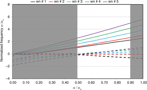
It is seen in Fig. 1 that although ω ₊ consistently shows a positive value with faster propagation speed for higher wavenumber n, ω ₋ displays much different behaviours. Specifically, the wavenumber n=1 has ω ₋<0 (i.e. retrograde propagation), the wavenumber 2 possesses ω ₋≈0, and all other higher wavenumbers have ω ₋>0. In addition, the retrograde mode for n=1 is most apparent at lower levels because of the stronger dependence of the square root on α in eq. (46). This suggests that one should look for retrograde waves at the lowest level for the azimuthal wavenumber 1, or at most wavenumber n=2. Note here the importance of both the baroclinicity (dα/dz)<0) and the atmospheric stratification H in determining the retrograde wave mode. Had H→∞ and dα/dz=0, eq. (41) would be identically equal to zero, and so one is left with the undetermined eq. (40). Apparently, such unique dependence of the wave frequency on the baroclinicity and the wavenumber mode is not seen in Kelvin's wave model due to Kelvin's assumption of R≪H and constant α with height.

It is of further significance that the relationship (46) imposes a specific condition on the radial scale of the inner-core perturbations. Indeed, substituting the dispersion relationship (46) into eq. (40) results in the following constraint:47

where the −sign is chosen in eq. (43) to ensure that the expansion (39) will correspond to a decreasing function of r within the inner-core region (i.e. ). Such − sign selection can be seen by noting that the larger value of n results in a larger Γ, and so D<0, and k can be negative only with the minus sign in (47).

Because of the condition (47), a larger azimuthal wavenumber would correspond to a smaller radial scale (i.e. 1/k~R/n) according to eq. (47). This implies that the faster waves corresponding to the higher wavenumber n will tend to have a smaller radial scale and they are mostly confined around R. For example, with azimuthal waves n=5, 1/k~R/5 and so the azimuthal wavenumber 5 would have quite small radial extend. Assume a typical RMW R=30 km, this indicates that any numerical simulation should have a horizontal resolution dx≤6 km so that the model could capture the existence of the wavenumber 5. Because of this constraint, simulations of wave-like propagation in the TC inner-core region need to have sufficiently high horizontal resolution to capture these high wavenumbers. Due to the dispersion relationship (46), it should be emphasised that the higher azimuthal wavenumbers may result in negative values under the squared root of (46) and allow for instabilities to develop, which are however outside the scope of wave propagation analyses in this study.

Thus far, the above wave analyses are applied only for waves inside the TC eye in the absence of both diabatic heating and frictional forcing. In practice, the propagation of inner-core waves is greatly interfered by moist processes in the eyewall, and propagation of adiabatic waves should be therefore limited within a short time window so that the adiabatic assumption can be applied. In the next section, we will examine in details some selected periods in a cloud-resolving numerical simulation of an idealised vortex in which episodes of retrograde waves are captured.

3. Numerical experiments

3.1. Experiment description

To examine potential existence of retrograde waves and their propagation inside the TC eye as obtained from the extension of Kelvin's wave model in Section 2, a high-resolution numerical simulation was carried out, using the latest version of the HWRF Tallapragada et al. (2014). This is a customised version of the Weather Research and Forecasting-Nonhydrostatic Mesoscale Model (WRF-NMM, Version 3.6) that is specifically aimed to operational TC forecasts and is currently maintained and operated in real-time by the US National Centers for Environmental Prediction.

The idealised configuration in this study was similar to that used in Gopalakrishnan et al. (2013) and Kieu et al. (2013) with triple nested domains on an f-plane located at 12.5°N. The model was initialised with a weak vortex that had the maximum azimuthal wind of 20 ms ⁻¹ at the surface and the RMW of 90 km in a quiescent environment. Unlike idealised configurations in the previous studies with 43 vertical levels, the simulation in this study had 61 vertical levels with a model top at 2 hPa instead of 50 hPa, and the three domains were configured at much higher horizontal resolution of ~8.1 km, 2.7 km, and 900 m. Such ultra-high horizontal resolution was used to allow for better resolved wave-like features inside the vortex centre. As discussed in the previous section, the approximation (39) for radially damped wave amplitudes would correspond to a smaller radial scale for higher azimuthal wavenumbers as given by eq. (47). Therefore, high resolution simulations are necessary to capture the wave propagation inside the vortex core. In addition to these changes, the sea surface temperature in this idealised configuration is set at 303.5 K instead of 302 K such that the simulated vortex can approach a higher maximum potential intensity limit. This is to ensure that the inner-core wave structure can be exposed more clearly, and the related linearisation can be best applied. Mote details about all other model physics configurations can be found in Bao et al. (2012) and Gopalakrishnan et al. (2013).

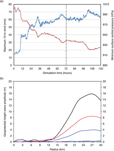
Before presenting analyses of retrograde waves, a number of remarks about potential difficulties with investigation of wave propagation in full-physics idealised simulations should be mentioned. First, the vortex development in a full-physics model never settles down to an absolute stationary state even if there exists a stable point (Kieu 2015) or a bounded maximum intensity attractor as pointed out recently in Kieu and Moon (2016). This is because three-dimensional models like the HWRF model are limited-area regional models that are heavily influenced by boundary conditions after some period of time. Hence, the requirement of a mean balanced vortex to be in an absolute steady state for the linearisation and the eigenmode expansion in Section 2.1 can never be fully satisfied. To ensure that this stationary requirement of the mean balance vortex is satisfied as much as possible, all wave analyses in this Section are carried out only for short time windows after 72 h into integration during which the model vortex is roughly in the stationary state (see Fig. 2a).

Fig. 2 (a) Time series of the maximum surface wind (blue) and the minimum surface pressure at the vortex centre (red) from the 120-h simulation of an idealised vortex using the HWRF model; and (b) radial profiles of the geopotential height wave amplitudes (m) valid at 72 h into integration for wavenumber 1 (black), wavenumber 2 (red), wavenumber 3 (blue), wavenumber 4 (cyan), and wavenumber 5 (purple). Dash line in the upper panel indicates the reference instant of time from which the wave analyses refer to.

The second issue with vortex simulations is that at the ultra-high horizontal resolution limit, the vortex centre is no longer uniquely defined, but constantly wobbling due to frequent emergence and disappearance of convective-scale anomalies and associated abnormally high vorticity centres. As a result, the storm centre based on either the minimum central pressure or the surface wind speed varies quickly from level to level and from time to time. Because of this strong variation in the storm centre, the wave decomposition around a storm centre often shows sudden changes in the wave structure during the wave evolution, and varies significantly at different vertical levels. This variation of the vortex centre makes it hard to track the evolution of waves continuously. In this study, the issue of the vortex centre fluctuation from the model high-frequency output is minimised by using a mass-weighted pressure distribution within a layer of 900–700 hPa to filter out all small-scale noises. In addition, the vortex centre is detected at every time step to avoid asymmetries caused by the wobbling of the vortex centre.

Along with the above difficulties, we should mention that full-physics models always contain moist processes by which deep convection constantly develops near the eyewall due to strong low level convergence. Even though the eye region is almost void of deep convection, new episodes of wave generation trigged near the eyewall region could produce strong impacts on subsequent propagation of waves inside the eye that neither the Kelvin's model nor the extension presented in Section 2 could take into account. Therefore, wave propagation inside the vortex eye can experience abrupt change, and it is hard to capture the full propagation of the inner-core waves continuously. Given those issues with full-physics simulations, our wave analysis in this section will be confined only within specific ad-hoc windows during which the retrograde propagation can be captured most evidently.

3.2. Results

Analyses in Section 2.2 suggest several important points about retrograde waves including (1) the retrograde waves should exist only for wavenumber 1 or at most wavenumber 2, (2) these waves are mostly realised between the middle level and the top of the planetary boundary layer where the mean balanced vortex is well approximated by the gradient wind balance, (3) the propagation speed of the retrograde waves is faster at lower levels, and (4) the wave amplitudes have to decay from the RMW inward such that the dispersion relationship (46) is valid. With these constraints, Fig. 2b shows the amplitudes of five azimuthal wavenumbers n=1,…,5 obtained from Fourier decomposition of the geopotential height perturbation Φ(r) valid at 72-h into integration. The inner-core wave amplitudes indeed decrease quickly with radius away from the RMW as an decaying function, with most of the wave projections on the azimuthal wavenumber 1, 2, and 3, and smaller projections onto the higher wavenumbers. This inward decrease of the wave amplitudes with radius to a good extent justifies the approximation (39) upon which the retrograde waves are derived.

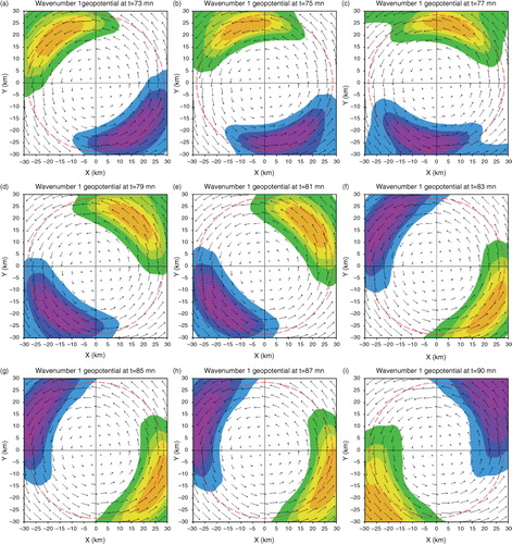
Given the above conditions for the existence of retrograde waves, Fig. 3 shows evolution of the azimuthal wavenumber n=1 obtained from the Fourier wave decompositions of Φ(r) after 72-h into integration at z=750 hPa inside the vortex core region. Because no retrograde waves are observed for higher wavenumbers n≥3, evolution of these higher wavenumbers is not provided herein. One notices in Fig. 3 the first evidence of the existence of the retrograde waves from minute 73 to minute 90 (with respect to the reference time origin at 72-h), which are all well confined near the vicinity of the RMW. Although it is difficult to find a time window that captures a full cycle of the retrograde wave propagation, estimation of the propagation speed in Fig. 3 shows that the wave propagates with a period of ~20 min, or equivalently ω≈5×10⁻³ s ⁻¹. Our examination of many other time windows showed that this anticyclonic propagation of the wavenumber 1 perturbation turns out to be a dominant mode at the vortex mature stage, albeit the full cycle of such wave propagation is not always apparent.

Fig. 3 Evolution of azimuthal wavenumber 1 geopotential height perturbation φ′(r,λ,z,t) (shaded) at 750 hPa from minute 73 to 90 relative to the time origin 72-h into integration (dashed line in Fig. 2a) in a 5-day simulation of an idealised vortex, using the HWRF model. All perturbations are normalised by the wave amplitude Φ(r=R) at each corresponding time. The time stamp denotes the minutes relative to the 72-h reference. Red circle denotes the RMW R at each instant of time, and vectors denote the mean tangential wind.

With the maximum surface wind of 61 ms ⁻¹ at the RMW of 30 km, the Rankine parameter at the surface α _s ≈2.0×10⁻³ s ⁻¹. This gives rise to a ratio ω/α _s ≈2.5, which ishigher than the theoretical ratio ω/α _s ≈1 seen in Fig. 1. Suchdiscrepancy in the wave frequency between the extended model presented in Section 2 and the numerical simulation could be related to various oversimplifications employed in the extended wave model or unknown nonlinear interaction among different wavemodes that the linearisation in Section 2 may not be applied. However, the fact the HWRF simulation could capture this retrograde mode is interesting, as it indicates that the inner-core region of TCs could in fact support such a retrograde wave mode, which to our knowledge has not been previously demonstrated.

While the retrograde wave mode is seen dominantly for wavenumber 1 for most time windows after the vortex attains its quasi-stationary stage, the fact that there exists two different wave propagating directions for each azimuthal wavenumber as implied by eq. (46) makes the wave analysis a bit more involved, because it is not known in advance what directions a wave will propagate. Unlike a perturbation of an arbitrary shape that can split into two smaller perturbations, each propagating in its own direction, the propagation of a sinusoidal eigenmode needs to ensure that the harmonic characteristics are well maintained, that is, wavenumber 1 has to be the same wavenumber 1 with time. From this physical perspective, the eigenmode perturbation at each instant of time can, therefore, travel in only one direction, which is determined by initial conditions. If both directions are allowed for the wavenumber 1, then one should expect to see realisation of cyclonic propagation of the wavenumber 1 at some other time windows as well.

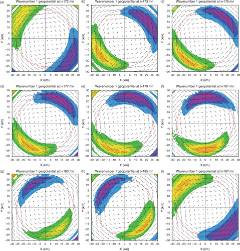
Indeed, Fig. 4 shows a similar time evolution of the wavenumber 1 perturbation as in Fig. 3, but for a different time window in which the cyclonic propagation of the wavenumber 1 is observed. One notices that this cyclonic wave propagation also has similar frequency as the retrograde mode with ω/α _s ≈1.8, which is again higher than the theoretical value of 1.2 seen in Fig. 1. Similar to the retrograde mode, we note that it is rare to observe a complete propagation of the cyclonic waves in our experiment. Most often, a wave propagates in one direction for about more than half of the cycle, and it suddenly changes its propagating direction for 5–10 min before resuming its previous propagation direction. This process alternatives every 20–30 min, with the overall dominance of the retrograde mode. In this regard, the existence of both the retrograde and the cyclonic propagating waves confirms the consistency of the wave analyses in Section 2.

Fig. 4 Similar to Fig. 3 but for different time window that exhibits the cyclonic propagation of the wavenumber 1.

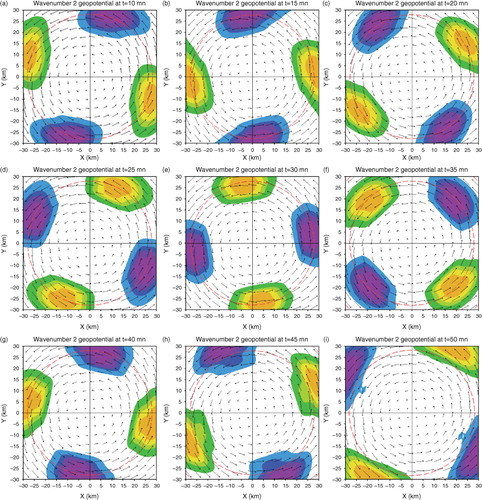
Regarding the wavenumber 2, the dispersion relationship displayed in Fig. 1 shows that there are also two wave modes that propagate in opposite directions similar to the wavenumber 1. However, the retrograde mode for the wavenumber 2 has too slow a speed that it is not likely that this retrograde mode can be realised in model simulations (the ratio ω/α _s for the wavenumber 2 retrograde between level 500 hPa and 850 hPa is ~0.1 as seen from the dashed red curve in Fig. 1). Indeed, our examination of the propagation of the wavenumber 2 does not capture evidence of the retrograde mode for the wavenumber 2 in all analyses. Instead, the wave propagation is dominantly cyclonic in most time windows.

Figure 5 shows an example of evolution of the wavenumber 2 between minute 10 and 50 after 72 h into integration, which captures a full cyclonic propagation of the wavenumber 2 with period of ~30 min. This wave period corresponds to the ratio ω/α _s ≈1.1, which is again different from the theoretical value of 2.2 as seen in Fig. 1. As a matter of fact, our probing of many different time windows shows that the wavenumber 2 cyclonic propagation is dominant and consistent at all time windows. Similar consistency is also seen for higher wavenumbers n≥2; all show persistent cyclonic propagation every time window (not shown). Unlike the wavenumber 1 that experiences abrupt changes in the propagating direction after some period of time, the cyclonic propagation is very smooth for n≥2 with no sudden change in the wave amplitudes or the direction during the entire course of propagation.

Fig. 5 Similar to Fig. 3 but for the wavenumber 2 from minute 10 to minute 50.

Despite some discrepancies in the exact values of the wave propagation speed between the extended wave model presented in Section 2 and the full-physics simulations, both the existence of the wavenumber 1 retrograde mode and the qualitative consistency in the propagation of the higher wavenumbers between the analytical model and the full-physics simulation give us confidence in the applicability of our extension of the Kelvin's wave model for the TC inner-core region.

4. Discussion and conclusion

In this study, the Kelvin's vortex wave model was extended for TC-like vortices to examine propagations of wave-like perturbations inside the TC inner-core region. It was found that the TC intrinsic baroclinicity and the atmospheric stratification introduce a strong constraint on the wave propagation inside the TC core, which is governed by a more involved dispersion relationship than the one that was obtained by Kelvin (1880) for a fluid column vortex whose aspect ratio is much larger than unity. By applying the Rankine-structure for the TC inner-core region, it was demonstrated that there exists unique simplification for which the inner-core wave eigenmodes can be described by a tractable dispersion relationship. Examination of this inner-core dispersion relationship showed that there are two different propagation modes for every azimuthal wavenumber. In particular, the azimuthal wavenumber n=1 possesses an intriguing retrograde mode associated with the strong baroclinicity of TCs, which is absent for all other higher wavenumbers n≥2. While this wavenumber 1 retrograde mode appears to be similar to the retrograde mode obtained in Kelvin's fluid column model, the retrograde mode in our extended model depends critically on the TC baroclinicity that Kelvin's model could not contain.

A numerical simulation of a TC-like vortex at an ultra-high horizontal resolution (900 m) using the full-physics HWRF model was conducted to look for such a particular retrograde wave mode. Decomposition of the TC inner-core wave spectrum at the quasi-stationary stage of the model vortex revealed that the retrograde wave mode is indeed realised for the azimuthal wavenumber 1 inside the core of the vortex. Furthermore, the propagation of simulated inner-core waves is qualitatively consistent with the analyses in our extended wave model, albeit the model simulated propagation speed is somewhat faster than what obtained in the extended wave model. Direct estimation of the retrograde wave propagation from the model high frequency output suggested that the period of the retrograde wavenumber 1 is ~20 min, and similarly for the cyclonic mode. The existence of both the retrograde and the cyclonic modes in this sense confirms the consistency of the wave analyses in our extended wave model for TC-like vortices. Despite the brief existence of this retrograde mode in the HWRF idealised simulations due to unaccounted strong wave coupling and moist processes, the emergence of such a retrograde wave mode is of significance, because they are potentially connected to the eyewall perturbations that account for different TC eye shape and instability, and possible formation of mesovortices associated with the eyewall instabilities.

5. Acknowledgements

This research was supported by a research fund provided by Indiana University and NOAA HFIP funding (NA16NWS4680026). Sincere thanks are extended to two anonymous reviewers whose detailed comments and suggestions have helped improve the quality and presentation of this work substantially. Numerical experiments were conducted on the High-Performance Computing system Big Red II of Indiana University, Bloomington.

Notes

1 Note that the log-pressure coordinate is defined with , where is the globally average temperature. Given , which is half of the tropospheric depth.

6. Appendix

A.1. Ring oscillation of the tropical cyclone inner core

The nature of the restoring force for the inner-core waves as obtained in eq. (46) can be most clearly seen by considering a mode of ring oscillation around the gradient wind balance for the core of a tropical cyclone (TC)-like vortex. Re-call the horizontal momentum equations:A1 A2

and assume that the mean states are in the gradient wind balance with a given geopotential distribution at a given radius of maximum wind R as follows:A3 A4 A5

Linearisation of eqs. (A1)–(A2) around the mean states (A3)–(A5) as results in a set of linearised equations:A6 A7

where the balance relationships (A3)–(A4) have been used in the above linearisation, and the ring oscillation mode has been assumed such that ∂u′/∂λ=∂v′/∂λ=0. Notice that for the inner-core of a TC-like vortex, such that , eqs. (A6)–(A7) are reduced toA8 A9

Combination of the above equations immediately shows that the TC inner core oscillates in the ring mode (i.e. no azimuthal dependence) at a frequency of ±Ω, which is identical to the dispersion relationship (46) when n=0 and dα/dz=0. Intuitively, this ring oscillation mode can be understood by imagining what would happen if one squeezes the TC inner-core radially a little bit inward. Because of the conservation of the absolute angular momentum, the tangential wind will increase and result in a stronger centrifugal force against the squeezing direction, thus pushing the inner core back to its original position. Likewise, if one pulls the inner core outward, the tangential wind will be reduced because of the conservation of the angular momentum again. As such, the pressure gradient force will dominate the reduced centrifugal force, and the inner core will therefore try to return to its original balance. Much like an inviscid water drop of mass m and surface tension σ will have an internal frequency , the inner core of a TC characterised by the RMW R and the maximum tangential wind V will experience a inherent frequency of Ω=V/R. From this perspective, the stiffness of the TC core demonstrates the nature of the inner-core oscillation under the gradient wind balance constraint (A3), which can be applied to both barotropic and baroclinic vortices. Of course, the baroclinicity modifies substantially the dispersion relationship as seen in Section 2.2, but the general physical mechanism behind such oscillation is intrinsically related to the ‘elasticity’ of the inner-core region of TC-like vortices as discussed in the main text.

References

- Bao J. W. , Gopalakrishnan S. G. , Michelson S. A. , Marks F. D. , Montgomery M. T . Impact of physics representations in the HWRFX on simulated hurricane structure and wind-pressure relationships. Mon. Weather Rev. 2012; 140: 3278–3299.
- Chen Y. , Yau M. K . Asymmetric structures in a simulated landfalling Hurricane. J. Atmos. Sci. 2003; 60: 2294–2312.
- Durran D. R . Improving the anelastic approximation. J. Atmos. Sci. 1989; 46: 1453–1461.
- Gopalakrishnan S. G. , Marks F. D. , Zhang J. A. , Zhang X. , Bao J. W. , co-authors . A study of the impacts of vertical diffusion on the structure and intensity of the tropical cyclones using the high-resolution HWRF system. J. Atmos. Sci. 2013; 70: 524–541.
- Guinn T. A. , Schubert W. H . Hurricane spiral bands. J. Atmos. Sci. 1993; 50: 3380–3403.
- Hack J. J. , Schubert W. H . Nonlinear response of atmospheric vortices to heating by organized cumulus convection. J. Atmos. Sci. 1986; 43: 1559–1573.
- Hendricks E. A. , McNoldy B. D. , Schubert W. H . Observed inner-core structural variability in Hurricane Dolly (2008). Mon. Weather Rev. 2012; 140: 4066–4077.
- Hogsett W. A. , Stewart S. R . Dynamics of tropical cyclone intensification: deep convective cyclonic left movers. J. Atmos. Sci. 2014; 71: 226–242.
- Holton J. R . An introduction to dynamic meteorology. 2004. Elsevier Academic Press, New York. 4th ed. (International Geophysics), p. 535.
- Kelvin L . Vibrations of a columnar vortex. Philos. Mag. 1880; 10: 155–168.
- Kieu C. Q. , Tallapragada V. , Hogsett W. A . On the onset of the tropical cyclone rapid intensification in the HWRF model. Geophys. Res. Lett. 2013; 9: 3298–3306.
- Kieu C. Q . Hurricane maximum potential intensity equilibrium. Q. J. Roy. Meteor. Soc. 2015; 141(692): 2471–2480. DOI: http://dx.doi.org/10.1002/qj.2556 .
- Kieu C. Q. , Moon Z . Hurricane Intensity Predictability. Bulletin of the American Meteorological Society. 2016. DOI: http://dx.doi.org/10.1175/BAMS-D-15-00168.1 .
- Kossin J. P. , Schubert W. H . Mesovortices in Hurricane Isabel. Bull. Am. Meteorol. Soc. 2004; 85: 151–153.
- Montgomery M. T. , Kallenbach R. J . A theory for vortex Rossby-waves and its application to spiral bands and intensity changes in hurricanes. Q. J. R. Meteorol. Soc. 1997; 123: 435–465.
- Montgomery M. T. , Vladimirov V. A. , Denissenko P. V . An experimental study on hurricane mesovortices. J. Fluid Mech. 2002; 471: 1–32.
- Nguyen L. T. , Molinari J. E . Evaluation of tropical cyclone centre identification methods in numerical models. 31st Conference on Hurricanes and Tropical Meteorology. 2014; CA: American Meteorological Society, San Diego. 94.
- Reasor P. D. , Montgomery M. T . Three-dimensional alignment and corotation of weak, TC-like vortices via linear vortex Rossby waves. J. Atmos. Sci. 2001; 58: 2306–2330.
- Schecter D. A . The spontaneous imbalance of an atmospheric vortex at high Rossby number. J. Atmos. Sci. 2008; 65: 2498–2521.
- Schecter D. A. , Montgomery M. T . Damping and pumping of a vortex Rossby wave in a monotonic cyclone: critical layer stirring versus inertia-buoyancy wave emission. Phys. Fluids. 2004; 16: 1334–1348.
- Schecter D. A. , Montgomery M. T . Conditions that inhibit the spontaneous radiation of spiral Inertia-gravity waves from an intense mesoscale cyclone. J. Atmos. Sci. 2006; 63: 435–456.
- Schubert W. H. , Montgomery M. T. , Taft R. K. , Guinn T. A. , Fulton S. R. , co-authors . Polygonal eyewalls, asymmetric eye contraction, and potential vorticity mixing in hurricanes. J. Atmos. Sci. 1999; 56: 1197–1223.
- Schubert W. H. , Rozoff C. M. , Vigh J. L. , McNoldy B. D. , Kossin J. P . On the distribution of subsidence in the hurricane eye. Q. J. R. Meteorol. Soc. 2007; 133: 595–605.
- Shea D. J. , Gray W. M . The hurricanes inner core region. I. Symmetric and asymmetric structure. J. Atmos. Sci. 1973; 30: 1544–1564.
- Tallapragada V. , Bernardet L. , Biswas M. K. , Gopalakrishnan S. , Kwon Y. , co-authors . Hurricane Weather Research and Forecasting (HWRF) Model: 2014 scientific documentation. NCAR Development Tested Bed Center Report. 2014. Online at: http://www.dtcenter.org/HurrWRF/users/docs/scientific_documents/HWRFv3.6a_ScientificDoc.pdf .
- Wang Y . Vortex Rossby waves in a numerically simulated tropical cyclone. Part I: overall structure, potential vorticity, and kinetic energy budgets. J. Atmos. Sci. 2010; 59: 1213–1238.
- Wilhelmson R. , Ogura Y . The pressure perturbation and the numerical modelling of a cloud. J. Atmos. Sci. 1972; 29: 1295–1307.
- Willoughby H. E . Inertia-buoyancy waves in hurricanes. J. Atmos. Sci. 1977; 34: 1028–1039.
- Willoughby H. E . The vertical structure of Hurricane Rainbands and their interaction with the mean vortex. J. Atmos. Sci. 1978; 35: 849–858.
- Willoughby H. E . Forced secondary circulations in hurricanes. J. Geophys. Res. 1979; 84: 3173–3183.
- Willoughby H. E , Marks F. D. , Feinberg R. J . Stationary and moving convective bands in hurricanes. J. Atmos. Sci. 1984; 41: 3189–3211.
- Yau M. K. , Liu Y. , Zhang D. L. , Yongsheng C . A multiscale numerical study of Hurricane Andrew (1992). Part VI: small-scale inner-core structures and wind streaks. Mon. Weather Rev. 2004; 132: 1410–1433.