Assessing atmospheric temperature data sets for climate studies

Abstract

Observed near-surface temperature trends during the period 1979–2014 show large differences between land and ocean, with positive values over land (0.25–0.27 °C/decade) that are significantly larger than over the ocean (0.06–0.12 °C/decade). Temperature trends in the mid-troposphere of 0.08-0.11 °C/decade, on the other hand, are similar for both land and ocean and agree closely with the ocean surface temperature trend. The lapse rate is consequently systematically larger over land than over the ocean and also shows a positive trend in most land areas. This is puzzling as a response to external warming, such as from increasing greenhouse gases, is broadly the same throughout the troposphere. The reduced tropospheric warming trend over land suggests a weaker vertical temperature coupling indicating that some of the processes in the planetary boundary layer such as inversions have a limited influence on the temperature of the free atmosphere. Alternatively, the temperature of the free atmosphere is influenced by advection of colder tropospheric air from the oceans. It is therefore suggested to use either the more robust tropospheric temperature or ocean surface temperature in studies of climate sensitivity. We also conclude that the European Centre for Medium-Range Weather Forecasts Reanalysis Interim can be used to obtain consistent temperature trends through the depth of the atmosphere, as they are consistent both with near-surface temperature trends and atmospheric temperature trends obtained from microwave sounding sensors.

• atmosphere
• climate
• temperature
• trend

1. Introduction

Records of global annual surface temperatures for the last 100 yr are an important data set often used in climate research, including the empirical assessment of climate sensitivity (Schwartz et al., 2014; Skeie et al., 2014; Lewis and Curry, 2015 and references therein). The reasons that near-surface temperatures (typically the temperature at 2 m above the ground) are normally used in climate studies are that such records are easily available, they exist for sufficiently long periods of time and they are the most relevant temperature data for impact studies.

In the past, near-surface temperature data sets have been produced (Hansen et al., 2010; Vose et al., 2012; Morice et al., 2012) and are widely used in the science community in determining climate sensitivity. However, near-surface temperature data, in particular over land, have several limitations that might compromise their usefulness for climate change studies. Firstly, near-surface temperature data are exposed to boundary layer effects such as sharp inversions. Secondly, they are influenced by urbanisation or other environmental changes that may compromise temperature trend calculations (Ren et al., 2008; Peng et al., 2012; Ryu and Baik, 2012). Thirdly, an incomplete coverage of surface temperature observations leaves areas of the globe unobserved, requiring methods of spatial interpolation (see Fig. 2b and c).

As atmospheric processes are vertically coupled through fast physical processes such as radiation and convection, temperature changes of the free atmosphere are expected to change in the same way as the near-surface temperatures (Manabe and Strickler, 1964). The temperature field of the free atmosphere is smoother than that near the surface as it is strongly exposed to large-scale horizontal mixing processes and is less affected by local surface conditions and the large differences in heat capacities near the surface (Davy and Esau, 2014), which can be considerable and lead to larger warming trends over dry land areas. It therefore seems more sensible to use tropospheric observations to determine more representative and more robust temperatures for the determination of climate sensitivity.

Temperatures from radiosondes become available from the early 1950s and have been used in atmospheric analyses since then. They constitute a major source of atmospheric information through the depth of the troposphere but are mainly restricted to extratropical land areas. Furthermore, early radiosonde data were obtained from a wide variety of instruments with different error statistics that made them less useful for climate studies. However, with the advent of global numerical weather prediction systems in the 1970s, more standardised methods have been implemented to control the radiosonde biases. A comprehensive assessment of radiosonde observation and its possible use in climate change studies can be found in Haimberger et al. (2012) and references therein.

With the implementation of a global observing system following the Global Weather Experiment in 1978 (Fleming et al., 1979), temperature information from satellite sounders has become available and now plays an essential role in numerical weather prediction. Extensive use has been made of microwave sounding data as a climate change indicator. Microwave radiation emanates from vibrations of the oxygen molecule, and from that, it is possible to infer the temperature from different layers of the atmosphere. The advantage with microwave observations is that they are virtually unaffected by clouds. Temperature estimates for different layers through the atmosphere have been compiled from a series of different space missions and data sets covering the period from 1979 until present and are generally available from two different groups (Christy et al., 2000; Mears and Wentz, 2009; Spencer et al., 2015).

An independent approach is to compare temperature from operational analyses as done in numerical weather prediction. As was originally proposed by Bengtsson and Shukla (1988), this requires a dedicated data assimilation system to avoid systematic biases. During the last decades, a number of re-analyses of past atmospheric observations have been undertaken (Onogi et al., 2007; Saha et al., 2010; Dee et al., 2011). In this study, we make use of recent re-analyses from the European Centre for Medium-Range Weather Forecasts (ECMWF). A main objective of this study is to explore whether the ECMWF Interim Reanalysis (ERAI) data set can reproduce credible temperature trends over a significant period of time.

However, global temperature records of the troposphere can only be used for limited time periods as data are only available globally with suitable accuracy since 1979 because of limited upper air observations from the Southern Hemisphere (SH) and the tropics before this date. Radiosonde data on their own have not been considered, because except when controlled and integrated into data assimilation, these data are subject to significant network and instrumentalchanges (Thorne et al., 2011). For this reason, we do not intend to use observations from the free atmosphere directly but instead use re-analyses, though we will also use temperatures derived from microwave sounders for comparison.

As part of the re-analysis process, the observational data undergo an advanced data bias control (Dee et al., 2011 and references therein). Satellite and aircraft data, assimilated by the re-analyses, have undergone systematic evaluation for the period after 1979, and we therefore believe that the re-analysis data can be considered as a reasonably independent robust source of tropospheric data (Simmons et al., 2014).

An alternative to using the tropospheric temperatures is to use sea surface temperatures (SSTs). The atmospheric temperature approximately 2 m above the ocean surface on average does not differ from the SST in a significant way, and temperature trends calculated over many years are expected to be the same as that of the SST.

In this article, we explore the temperature trend of the free atmosphere using re-analyses as well as satellite Microwave Sounding Unit (MSU) observations and compare these with the surface temperature trend. We focus the assessment on the period 1979–2014 as for this period we have reliable records of global surface observations as well as observations of the troposphere from radiosondes, satellite soundings and aircraft reports, which are incorporated into the re-analyses.

The article continues in Section 2 where we describe and comment on the data used, their possible limitations and usefulness for this kind of investigation. In Section 3, we present the results, and in Section 4, the findings of the article and their possible implications in assessing climate sensitivity as a consequence of greenhouse gases and other global radiative forcing of the climate system are discussed.

2. Data and methodology

For surface temperature data, the Goddard Institute for Space Studies (GISS) Surface Temperature Analysis (GISTEMP) data (Hansen et al., 2010) and the HadCRUT4 data set (Morice et al., 2012) are used. These data are based on monthly averaged data from synoptic surface stations analysed by different standard algorithms and include temperatures over most ocean areas. HadCRUT4 uses a reduced number of records and avoids interpolation into data sparse regions with the consequence that there is hardly any data over the Arctic Ocean, or in some tropical land areas, and with reduced data poleward of 45°S. The GISTEMP data set employs an analysis using a broad structure function and is consequently able to provide an almost homogeneous data set.

The re-analysis data used is ERAI (Dee et al., 2011). It has been produced by assimilating synoptic, aircraft and remotely sensed data using a 4-dimensional variational (4D-Var) data assimilation system with a 12-hour cycle. While the method to assimilate observations is fixed in the production of the re-analyses, the available observations used have undergone changes as new types of observations have been added over time and some observations may similarly have disappeared. This might imply a possible inconsistency or bias which means that ERAI must be examined carefully in this respect (e.g. Bengtsson et al., 2004), although inter-comparisons between surface temperature trends for land areas with HadCrut show virtually identical results (Simmons et al., 2004). For this study, tropospheric temperature data from ERAI between 400 and 700 hPa and at the surface (2 m) are used.

The data period covered using ERAI is from 1979 to 2014, since the period offers a more diverse range of observations, providing better global coverage, in particular from satellites, and also including observations from radiosondes and aircraft. This allows temperature for the global atmosphere to be determined with an estimated accuracy of about 0.2 °C for the global annual average (Hansen et al., 2010; Morice et al., 2012; Vose et al., 2012). Nevertheless, there are still remaining problems in estimating temperature trends as many surface observations have systematic biases including effects of urbanisation and changes in land surface conditions. For an in-depth discussion of the issues, see Jones (2016) and references therein. Other problems occur due to systematic errors in major observing systems such as satellites and aircraft, and great care must be exercised to identify biases and other observational deficiencies. For a comprehensive description, see Simmons et al. (2014).

The results of tropospheric temperature trends from the re-analyses will also be contrasted with temperature trends obtained from satellite passive microwave data. Microwave sounding from operational polar orbiting satellites has been regularly used since 1978 to measure atmospheric temperature in different spectral bands (e.g. Christy et al., 2000; Mears and Wentz, 2009). For the period 1975–2005, the MSU and, from 1998, the Advanced Microwave Sounding Unit (AMSU) were used. Significant efforts have been undertaken to combine the data from the different series of satellites into homogeneous data sets. Two data sets commonly used have been developed by the University of Alabama in Huntsville (UAH) (Christy et al., 2000) and by Remote Sensing Systems (RSS) (Mears and Wentz, 2009). These are regularly updated on a monthly basis. Here, we use the temperature profile of the lower troposphere (temperature lower troposphere [TLT]), broadly representing the temperature between the surface and 300 hPa with the largest contribution between 850 and 500 hPa. For UAH, we have used the latest version 6.0 released in April 2015 (Spencer et al., 2015).

Firstly, we assess, the first and most important issue, the difference in the surface warming over land and sea separately and contrast this with the corresponding warming in the troposphere as determined from the re-analysis. We do this by investigating the temperature trends in the re-analysis obtained from the thickness between 400 and 700 hPa and contrasting this with the surface temperature trends, based on the surface observations and the satellite-derived TLT. The thickness represents the mean temperature of a tropospheric layer with the depth of approximately 3000 m or about a third of the tropospheric air mass. Except for minor areas, the lowest pressure level is well above the ground and the upper level is still in the troposphere. Secondly, we highlight a number of differences in available surface data sets and discuss aspects that might affect their general use.

All temperature trends have been calculated based on annual averages, and the effect of serial correlation has been considered following the method used by Santer et al. (2000); however, the serial correlation has been found to be minor.

3. Results

3.1. Surface temperature trends

Figure 1 shows the globally averaged surface temperature trend based on ERAI, GISTEMP and HadCRUT4. All global and regional averages have been computed using area weighting. These show that there are large interannual variations and an indication of a steeper trend prior to 1997. The results from GISTEMP and HadCRUT4 are practically identical despite the fact that they are computed from data with a different areal coverage (see Fig. 2b and c). The temperature trend from ERAI is slightly lower (Table 1). This is related to the low SST trend discussed below. Over land, the temperature trends from the three different data sets are practically identical (Table 1) in spite of the fact that the ERAI data are calculated from analysed parameters.

Fig. 1 Global mean surface temperature trends for the period 1979–2013 for ERAI, GISSTEMP and HadCRUT4.

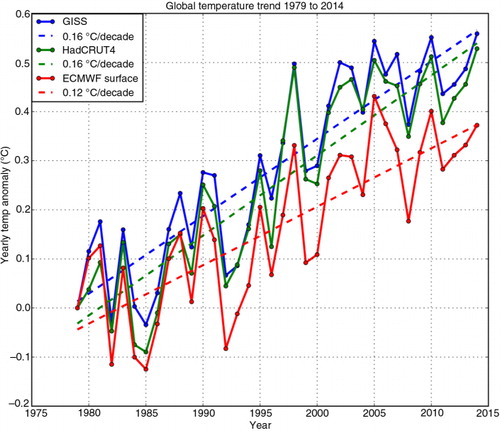
Fig. 2 Surface temperature trends for the period 1979–2013 for (a) ERAI, (b) GISSTEMP and (c) HadCRUT4. Significant trends at the 95 % level are indicated by the open circles.

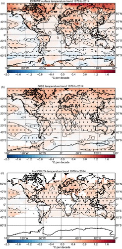
Table 1. Surface temperature trends in °C/decade for the period 1979–2014

Area surface	ERAI	GISS	HAD
Glob. land	0.26±0.06	0.25±0.05	0.27±0.06
Glob. ocean	0.06±0.02	0.12±0.02	0.12±0.02
Glob. all	0.12±0.03	0.16±0.03	0.16±0.03
NH land	0.33±0.07	0.31±0.07	0.31±0.07
NH ocean	0.14±0.03	0.18±0.03	0.16±0.03
NH all	0.21±0.04	0.23±0.04	0.22±0.04

Values are for surface temperature from ERAI, GISTEMP and HadCRUT4. Confidence intervals are at 95 % level. For further information see text.

The geographical distribution of the surface temperature trends from ERAI, GISTEMP and HadCRUT4 (Fig. 2) differs locally but when integrated over large domains, the differences are minor (Fig. 1). The surface temperature trend of the 36-yr period exhibits large differences between land and ocean with values over land considerably larger than those for ocean areas (Table 1). Moreover, the ocean areas of the Northern Hemisphere (NH) have on average a stronger warming trend than that of the SH (not shown). A large warming is also observed in the Arctic Ocean region presumably related to reduced sea ice cover in summer and autumn.

SST data sets are compiled by combining both ship and satellite data. Before 1982, they were based on ship measurements alone (e.g. Rayner et al., 2006). After 1982, satellite SST data are added (e.g. Reynolds et al., 2002). Detailed information can be found in Hansen et al. (2010) for GISS, Morice et al. (2012) for HadCRUT4 and Dee et al. (2011) for ERAI.

The SST trends are lower for ERAI (Table 1). This is mainly related to the SH and the period prior to 2001 (not shown) and is presumably related to the treatment of sea ice in the different data sets (see Hansen et al. (2010), Morice et al. (2012) and Simmons et al. (2014) for a more in-depth discussion). Between 2001 and 2013, the SST trends were virtually identical and close to zero for the three data sets (not shown).

It cannot be excluded that biases in the SST data, through the data assimilation process in ERAI, may have influenced the upper air temperature trends, although the assimilation of satellite temperature soundings and other upper air observations, which are independent observations, make this unlikely. A systematic and automated bias control is included in the ERAI data assimilation (Dee and Uppala, 2009). The temperature trend for the troposphere is the same as that for the sea surface after 2001 for ERAI, suggesting a slight cold bias in the period prior to 2001 (not shown).

3.2. Upper air temperature trends

We primarily examine the temperature trend for the 700–400 hPa layer that can be considered as a representative layer for the troposphere. For most of the globe, it is unaffected by boundary layer and local surface conditions. As can be seen from Table and 2 , the upper air trend is significantly smaller than the surface temperature trend for land areas but more or less the same as that for ocean areas. The global upper air temperatures undergo considerable interannual temporal variations with marked global warming during El Nino events such as 1997/1998 and 2010 and distinct cooling during La Nina events such as 1999/2000 and 2008 (Fig. 3).

Fig. 3 Global mean upper air temperature trends for the period 1979–2013 for ERAI, UAH and RSS.

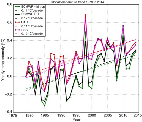
Table 2. Temperature trends in °C/decade for the period 1979–2014

Area tropospheric	ERAI layer mean 700–400 hPa	UAH TLT	RSS TLT
Glob. land	0.09±0.06	0.19±0.06	0.17±0.06
Glob. ocean	0.11±0.06	0.08±0.04	0.11±0.04
Glob. all	0.11±0.06	0.11±0.05	0.12±0.05
NH land	0.12±0.07	0.19±0.06	0.19±0.07
NH ocean	0.13±0.06	0.09±0.05	0.15±0.05
NH all	0.13±0.06	0.13±0.05	0.16±0.05

Values are given for the mean temperature trend for the layer 700–400 hPa. It also shows the TLT values from MSU data for UAH and RSS, respectively. NH refers to the area 0–90°N. Note that TLT is influenced by surface data over land. Confidence intervals are at 95 % level.

Figure 4a shows the spatial variation in temperature trends for the 700–400 hPa layer. As for the surface temperature trend, there are significant regional differences but the pattern is much broader in structure, and there are no significant changes between ocean and land areas. There are major parts of the globe where the local trends are not significant at the 95 % level. The strongest warming is found over the northwest Pacific and the area around Greenland, areas where the natural variability is high (not shown). This is further supported from recent climate ensemble simulations (Kay et al., 2015) as well as from model simulations by Hunt and Elliot (2006) suggesting that the time period of 36 yr is probably too short to quantify robust regional trends.

Fig. 4 (a) ERAI temperature trend for the mean temperature of the layer 700–400 hPa, (b) UAH TLT trend and (c) RSS TLT trend. Significant trends at the 95 % levels are indicated by the open circles.

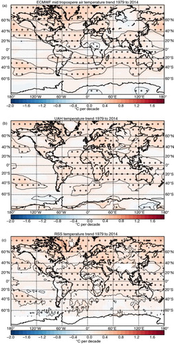
Figure 4b and c show the results for the trend of the MSU TLT (see Christy et al., 2000; Mears and Wentz, 2009) from UAH and RSS, respectively. As TLT is a weighted temperature contribution from practically all tropospheric levels (e.g. Bengtsson and Hodges, 2011), it cannot be directly compared with the 700–400 hPa thickness layer but should mainly represent the mid-troposphere except over land, where the surface emissivity becomes a larger portion of the signal so that the measurements represent a lower overall average altitude. The MSU temperature data are in broad agreement with ERAI – but are incomplete at higher latitudes and show higher spatial variability than the ERAI data, in particular over land. There are reasonable similarities over ocean regions but differences over land. There are also differences between the UAH and the RSS TLT, particularly over land and at high latitudes (Fig. 4b and c). There are minor differences in the coverage, but we judge that these are probably insignificant for averaging the trend over global and hemispheric domains. As can be seen from Table and 2 , results over the oceans are broadly consistent with a similar result through the troposphere for the MSU data as well as ERAI indicating the same trends throughout the lower and mid-troposphere.

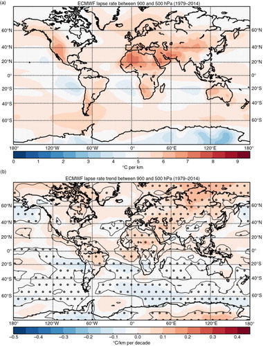
In order to get a better understanding of the relatively large surface temperature trend over land compared to the smaller temperature trend in the mid-troposphere, we have calculated the mean lapse rate between 900 and 500 hPa, as well as the trend in the lapse rate (Fig. 5). Statistically, significant lapse rate changes at the 95 % level are indicated by dots. It can be seen that the lapse rate is largest over the land regions, in particular over areas with desert or semi-desert regions. The trend in lapse rates is significant over most land areas.

Fig. 5 (a) ERAI mean lapse rate and (b) lapse rate trend between 900 and 500 hPa. Significant trends at the 95 % levels are indicated by the open circles.

3.3. Temperature trends through the full depth of the atmosphere

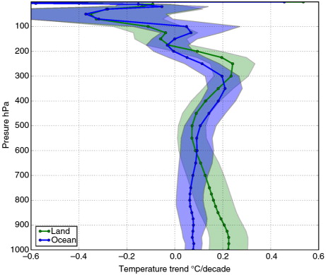
The ERAI temperature data are available at high vertical resolution between 1000 and 1 hPa. Figure 6 shows the global decadal trends for all levels. The upper levels that are in the stratosphere show a general cooling trend, while a warming trend is found at all levels in the troposphere. The largest warming occurs everywhere in the upper troposphere around 400–300 hPa but also in the lowest part of troposphere over land areas. The minimum warming occurs around 500 hPa.

Fig. 6 ERAI global decadal temperature trends for all vertical levels 1000 – 1 hPa. Significant trends at the 95 % level are indicated by shading.

By having access to all the levels of ERAI, it is also possible to calculate the equivalent MSU radiation using weighting functions for individual pressure levels kindly provided by J Christy. The result is summarised in Table 3. For easier comparison, we also repeat the UAH and RSS values from Table 2. The global values for land and ocean separately are in good agreement especially ERAI and RSS. UAH trends over ocean areas are lower.

Table 3. The same as Table 2 but where the ERAI layer mean has been replaced by TLT calculated from the ERAI equivalent to a MSU sounder from the real atmosphere

Area tropospheric	ERAI TLT	UAH TLT	RSS TLT
Glob. land	0.16±0.06	0.19±0.06	0.17±0.06
Glob. ocean	0.10±0.05	0.08±0.04	0.11±0.04
Glob. all	0.12±0.07	0.11±0.05	0.12±0.05
NH land	0.21±0.07	0.19±0.06	0.19±0.07
NH ocean	0.16±0.06	0.09±0.05	0.15±0.05
NH all	0.18±0.06	0.13±0.05	0.16±0.05

The trends in Table and 2 all include confidence intervals at the 95 % level, corrected for serial correlation using a method suggested by Santer et al. (2000). The additional effect of serial correlation is minor because the temperature trends are calculated from annual averages and the trends refer to a period of 36 yr.

4. Discussions and conclusions

The results show that surface air temperature changes over land are significantly larger than those over the oceans. This is to be expected because of the limited heat capacity of land surfaces compared to the ocean as was already demonstrated in early climate simulation studies (Manabe and Strickler, 1964). Other possibilities could be associated with changes in surface albedo such as reduced snow cover in winter that will act as a positive feedback factor. There is also the possibility that urbanisation effects have been underestimated as has been suggested from some studies (Hung et al., 2006; Peng et al., 2012; Ryu and Baik, 2012). It could also be that ERAI has a systematic cold bias in the free atmosphere over land, but this is not very likely, as we do not see this over the oceans. Furthermore, this is unlikely as the calculated TLT from the re-analyses agrees with the TLT measured from MSU (Table 3).

It has recently been shown by Gleisner et al. (2015) using radio occultation data that from the Global Navigation Satellite System, these data support the MSU data and thus indirectly the re-analyses from ERAI.

The surface temperature trend over land stands out. It is about twice as large as the temperature trend of the mid-troposphere. In the mid-troposphere, the trend is similar to that over the ocean. A possible explanation could be the drying out of the land surface leading to reduced fluxes of water vapour from the ground accompanied by a larger lapse rate.

Another area with a large warming trend is in the Arctic, most likely due to reduced sea ice cover in summer and autumn. The Arctic warming trend is most pronounced in ERAI (Fig. 2a) with the largest values in the Russian sector.

Such values are consequently not a direct effect of increasing greenhouse gases. It is most likely due to reduced sea ice in summer and autumn that in turn can be a secondary effect of climate warming but with no apparent warming response at upper levels (compare Fig. 2a and 4a). Another response can be seen in subtropical latitudes, 20–40°, in both hemispheres (Fig. 5a). This is what is to be expected generally in dry and hot areas where the vertical temperature profile closely follows the dry adiabatic stratification. It is also interesting to note that the trend in the lapse rate is also increasing, meaning that the temperature difference between the surface and the mid-troposphere is increasing during the period (Fig. 5b). This increase occurs over most land areas including higher latitudes, the Arctic and Antarctic regions. Weather situations in high latitudes with reduced inversions could add to such a development. Typical of the Arctic climate are pronounced boundary layer inversions that at low solar angles often persist during the day. A more detailed examination of the vertical structure of the trend (not shown) shows that the near-surface temperature trend is approximately 2.5 times larger than that in the mid-troposphere. The difference is largest over ocean suggesting an additional contribution from reduced sea ice coverage. The reason for the enhanced warming of the boundary layer is not clear but is probably a combination of circulation changes and surface boundary conditions. For additional discussions, see Graversen et al. (2014) and Pithan and Mauritsen (2014) and references therein.

In the situation of a sustained warming or cooling of the climate caused by changes in radiative forcing (greenhouse gases, solar irradiation or volcanic eruptions), the temperature change through the troposphere should stay approximately the same for all vertical levels because of the strong vertical coupling due to fast atmospheric processes such as convection and constant large-scale horizontal mixing (Manabe and Strickler, 1964). In the case of net positive forcing, the tropospheric warming is expected to be slightly larger in the upper troposphere. This is because of the influence of the moist adiabatic lapse rate at higher tropospheric temperatures. However, with present minor temperature changes and data limitations, this cannot be uniquely determined.

The minimum temperature increase in the mid-troposphere, as suggested from ERAI and most clearly indicated over land (Fig. 6), is somewhat puzzling. Comparison with GCM simulations, to be reported elsewhere, shows that this does not occur in model simulations. According to Simmons et al. (2014), the contrast between radiosondes and the re-analyses is about 0.1 °C or better below 500 hPa for the period as a whole and consequently the calculated trend values are well supported. A possible explanation might be that model simulations have difficulties to handle the magnitude of different convective processes over land including the effect of limited horizontal resolution preventing a more realistic parameterization of mixed dry and moist convection.

The ERAI data are not free from systematic errors, which may affect trends. However, the large amount of different observations now used in the ERAI data assimilation suggest (see Simmons et al., 2014 and references therein) that the biases caused by changing observations over time, as pointed out by Bengtsson and Hodges (2011), are unlikely to corrupt the trend calculations and in any case not more than trends calculated from one set of specific observations.

We have highlighted in this article the problem with surface temperature trends over land. However, it is important to point out that SST trends are also problematic, particularly prior to the availability of reliable satellite observations. Available data sets have been composed by merging different types of observations in a partly subjective way that is not possible to fully reproduce.

We have also used available independent MSU data provided by UAH and RSS. There are minor differences between the two data sets as well as the corresponding values calculated from the vertical temperature profiles of ERAI (Table 3). Comparing TLT of UAH and RSS with that calculated from ERAI shows a close agreement with the exception of the ocean TLT trends for UAH that are lower than the other two.

Tropospheric temperature trends are affected by gradual changes mainly in space observations both with respect to quality and coverage, but further improvements are expected with new re-analyses having more advanced bias control. We therefore strongly suggest that tropospheric temperature trends from re-analyses should replace surface temperature trends in future climate validation studies. If we use the temperature trend of the layer 700–400 hPa or any other similar measure, instead of the surface temperature trend, then this is probably a better representation of the global tropospheric temperature and presumably a more robust quantity to assess climate change.

5. Acknowledgements

The authors gratefully acknowledge access to available data sets from University of Alabama, RSS, GISS, UK Met Office and ECMWF.

References

- Bengtsson L., Hagemann S., Hodges K. I. Can climate trends be calculated from re-analysis data?. J. Geophys. Res. 2004; 109: 11111. http://dx.doi.org/10.1029/2004JD004536.
- Bengtsson L. , Hodges K. I . On the evaluation of temperature trends in the tropical troposphere. Clim. Dyn. 2011; 36: 419–430.
- Bengtsson L. , Shukla J . Integration of space and in situ observations to study global climate change. Bull. Am. Meteorol. Soc. 1988; 69: 1130–1143.
- Christy J. R. , Spencer R. W. , Braswell W. D . MSU tropospheric temperatures: data set construction and radiosonde comparisons. J. Atmos. Ocean. Technol. 2000; 17: 1153–1170.
- Davy R. , Esau I . Surface air temperature variability in global climate models. Atmos. Sci. Lett. 2014; 15: 13–20.
- Dee D. P. , Uppala S . Variational bias correction of satellite radiance data in the ERA-Interim reanalysis. Quart. J. Roy. Meteor. Soc. 2009; 135: 1830–1841.
- Dee D. P. , Uppala S. M. , Simmons A. J. , Berrisford P. , Poli P. , co-authors . The ERA-Interim re-analysis: configuration and performance of the data assimilation system. Quart. J. Roy. Meteor. Soc. 2011; 137: 553–597.
- Fleming R. G. , Kaneshige T. M. , McGovern W. E . The global weather experiment 1. The observational phase through the first special observing period. Bull. Am. Meteorol. Soc. 1979; 60: 649–661.
- Gleisner H., Thejll P., Christiansen B., Nielsen J. K. Recent global hiatus dominated by low-latitude temperature trends in surface and tropospheric data. Geophys. Res. Lett. 42: 510–517. http://dx.doi.org/10.1002/2014GL062596.
- Graversen R. , Langen P. , Mauritsen T . Polar amplification in CCSM4: contributions from the lapse rate and surface albedo feedbacks. J. Clim. 2014; 27: 4433–4450.
- Haimberger L., Tavolato C., Sperka S. Homogenization of the global radiosonde temperature dataset through combined comparison with reanalysis background series and neighboring stations. J. Clim. 2012; 25: 8109–8130. http://dx.doi.org/10.1175/JCLI-D-11-00668.1.
- Hansen J., Ruedy R., Sato M., Lo K. Global surface temperature change. Rev. Geophys. 2010; 48: 4004. http://dx.doi.org/10.1029/2010RG000345.
- Hung T. , Uchihama D. , Ochi S. , Yasuoka Y . Assessment with satellite data of the urban heat island effects in Asian mega cities. Int. J. Appl. Earth Obs. Geoinf. 2006; 8: 34–48.
- Hunt B. G. , Elliot T. I . Climatic trends. Clim. Dyn. 2006; 26: 567–585.
- Jones P . The reliability of global and hemispheric surface temperature records. Adv. Atmos. Sci. 2016; 33: 269–282.
- Kay J. E., Deser C., Phillips A., Mai A., Hannay C., co-authors. The Community Earth System Model (CESM) large ensemble project: a community resource for studying climate change in the presence of internal climate variability. Bull. Am. Meteorol. Soc. 2015; 96: 1333–1349. http://dx.doi.org/10.1175/BAMS-D-13-00255.1.
- Lewis N., Curry J. A. The implications for climate sensitivity of AR5 forcing and heat uptake estimates. Clim. Dyn. 2015; 45: 1009–1023. http://dx.doi.org/10.1007/s00382-014-2342-y.
- Manabe S. , Strickler R. F . Thermal equilibrium of the atmosphere with a convective adjustment. J. Atmos. Sci. 1964; 21: 361–385.
- Mears C. A., Wentz F. J. Construction of the remote sensing systems V3.2 atmospheric temperature records from the MSU and AMSU microwave sounders. J. Atmos. Ocean. Technol. 2009; 26: 1040–1056. DOI: http://dx.doi.org/10.1175/2008JTECHA1176.1.
- Morice C. P., Kennedy J. J., Rayner N. A., Jones P. D. Quantifying uncertainties in global and regional temperature change using an ensemble of observational estimates: the HadCRUT4 dataset. J. Geophys. Res. 2012; 117 D08101. DOI: http://dx.doi.org/10.1029/2011JD017187.
- Onogi K., Tsutsui J., Koide H., Sakamoto M., Kobayashi S., co-authors. The JRA-25 reanalysis. J. Meteorol. Soc. Japan. 2007; 85: 369–432. DOI: http://dx.doi.org/10.2151/jmsj.85.369.
- Peng S. , Piao S. , Ciais P. , Friedlingstein P. , Ottle C. , co-authors . Surface urban heat island across 419 global big cities. Environ. Sci. Technol. 2012; 46: 696–703.
- Pithan F. , Mauritsen T . Arctic amplification dominated by temperature feedbacks in contemporary climate models. Nat Geosci. 2014; 7: 181–184.
- Rayner N. A., Brohan P., Parker D. E., Folland C. K., Kennedy J. J., co-authors. Improved analyses of changes and uncertainties in sea-surface temperature measured in situ since the mid-nineteenth century: the HadSST2 data set. J. Climatol. 2006; 19: 446–469. DOI: http://dx.doi.org/10.1175/JCLI3637.1.
- Ren G. , Zhou Y. , Chu Z. , Zhou J. , Zhang A. , co-authors . Urbanization effects on observed surface air temperature trends in North China. J. Climatol. 2008; 21: 1333–1348.
- Reynolds R. W. , Rayner N. A. , Smith T. M. , Stokes D. C. , Wang W . An improved in situ and satellite SST analysis for climate. J. Climatol. 2002; 15: 1609–1625.
- Ryu Y.-H. , Baik J.-J . Quantitative analysis of factors contributing to urban heat island intensity. J. Appl Meteorol. Climatol. 2012; 51: 842–854.
- Saha S., Moorthi S., Pan H.-L., Wu X., Wang J., co-authors. The NCEP climate forecast system reanalysis. Bull. Am. Meteorol. Soc. 2010; 91: 1015–1057. DOI: http://dx.doi.org/10.1175/2010BAMS3001.1.
- Santer B. D. , Wigley T. M. , Boyle J. S. , Gaffen D. J. , Hnilo J. J. , co-authors . Statistical significance of trend differences in layer-average atmospheric temperature time series. J. Geophys. Res. 2000; 105: 7337–7356.
- Schwartz S. E. , Charlson R. J. , Kahn R. , Rodhe H . Earth's climate sensitivity: apparent inconsistencies in recent assessments. Earths Future. 2014; 2: 601–605.
- Simmons A. J., Jones P. D., da Costa Bechtold V., Beljaars A. C. M., Kållberg P. W., co-authors. Comparison of trends and low-frequency variability in CRU, ERA-40 and NCEP/NCAR analyses of surface air temperature. J. Geophys. Res. 2004; 109 D24115. DOI: http://dx.doi.org/10.1029/2004JD005306.
- Simmons A. J. , Poli P. , Dee D. P. , Berrisford P. , Hersbach H. , co-authors . Estimating low-frequency variability and trends in atmospheric temperature using ERA-Interim. Quart. J. Roy. Meteorol. Soc. 2014; 140: 329–353.
- Skeie R. B. , Berntsen T. , Aldrin M. , Holden M. , Myhre G . A lower and more constrained estimate of climate sensitivity using updated observations and detailed radiative forcing time series. Earth Syst. Dynam. 2014; 5: 139–175.
- Spencer R.W., Christy J.R., Braswell W.D. Version 6.0 of the UAH temperature dataset. 2015. Online at: http://www.drroyspencer.com/2015/04/version-6-0-of-the-uah-temperature-dataset-released-new-lt-trend-0-11-cdecade/.
- Thorne P. W., Brohan P., Titchner H. A., McCarthy M. P., Sherwood S. C., co-authors. A quantification of uncertainties in historical tropical tropospheric temperature trends from radiosondes. J. Geophys. Res. 116 D12116. DOI: http://dx.doi.org/10.1029/2010JD015487.
- Vose R. S. , Arndt D. , Banzon V. F. , Easterling D. R. , Gleason B. , co-authors . NOAA's merged land–ocean surface temperature analysis. Bull. Am. Meteorol. Soc. 2012; 93: 1677–1685.