Seasonal variations in atmospheric responses to oceanic eddies in the Kuroshio Extension

Abstract

Analyses using high-resolution satellite observations reveal distinct seasonal variations in atmospheric responses to oceanic eddies in the Kuroshio Extension (KE) region, characterised by much stronger surface wind speed and heat flux responses in the cold seasons (winter and spring) than in the warm seasons (summer and autumn). Cloud liquid water and rain rate also display seasonally dependent characteristics, with more deficit (surplus) in winter than in summer over the cold (warm) oceanic eddies. CFSR (Climate Forecast System Reanalysis) data can well reproduce these seasonal variations in surface atmospheric responses to the eddies in the KE region, albeit with much weaker responses in surface wind speed and with stronger responses in latent heat flux in comparison with the results based on satellite observations. In addition, the CFSR data also reveal remarkable seasonal variations in tropospheric responses, with eddy-induced wind speed (vertical velocity) anomalies reaching as high as 900 hPa (800 hPa) in winter, while they only occur near the sea surface in summer. The Weather Research and Forecast (WRF) model is applied to study the seasonal variations in atmospheric responses to idealised oceanic eddies. The model successfully simulates the seasonal variations in atmospheric responses to an idealised warm eddy in terms of wind speed, heat flux, marine atmospheric boundary layer (MABL) height and vertical velocity in both seasons. Both the CFSR data and the model simulations indicate that the seasonal variations in atmospheric responses to oceanic eddies can be attributed to the variations in background atmospheric stability during different seasons.

• Kuroshio Extension
• oceanic eddy
• seasonal variation
• heat flux
• marine atmospheric boundary layer
• vertical velocity
• Weather Research and Forecast model

1. Introduction

Air-sea interaction associated with oceanic fronts exhibits positive correlation between sea surface temperature (SST) and wind speed, indicative of the active role of ocean in forcing the atmosphere (Liu et al., 2000; Hashizume et al., 2001; Xie et al., 2002; Nonaka and Xie, 2003; O'Neill et al., 2003, 2005; Chelton et al., 2004; Xie, 2004; Tokinaga et al., 2005; Liu et al., 2007; Minobe et al., 2008, 2010). This contrasts with the negative correlation between surface wind speed and SST on a basin scale in the extratropics, which is due to the atmospheric forcing onto the ocean via surface heat fluxes and Ekman currents in response to changes in surface wind speed, surface air temperature and surface humidity, interpreted as evidence that the atmosphere is driving the ocean (Namias and Cayan, 1981; Wallace et al., 1990).

Some studies focus on the atmospheric responses to long-lived or stationary oceanic eddies (White and Annis, 2003; Bourras et al., 2004). They reported that cold (warm) eddies enhance (reduce) the stability of the marine atmospheric boundary layer (MABL) and decrease (increase) surface wind, with lower (higher) latent and sensible heat fluxes.

Compared with the extensive research on atmospheric responses to stationary oceanic fronts and stationary oceanic eddies, studies on atmospheric responses to transient oceanic eddies based on large populations of eddies in specific regions are relatively new (Frenger et al., 2013; Ma et al., 2015), though eddy activity is a dominant phenomenon in the turbulent upper ocean (Chelton et al., 2007; Qiu and Chen, 2010). By examining atmospheric responses to more than 600,000 transient eddies in the Southern Ocean, Frenger et al. (2013) found a reduction (increase) in surface wind speed, and declines (increases) in cloud fraction, water content and rainfall over the cold (warm) eddies. Ma et al. (2014) examined atmospheric responses to two typical long-lived oceanic eddies (a cyclonic eddy and an anticyclonic one) in the Kuroshio Extension (KE) region. Figure 1 clearly shows that eddy activity is energetic over the KE region, making it an ideal area for eddy-related study. They found that positive correlation between SST and surface wind speed is evident in dynamic composites and that mesoscale oceanic eddies can exert their influences on atmospheric transient disturbance intensity. More recently, Ma et al. (2015) investigated the atmospheric responses to 35,000+ oceanic eddies in the KE region during the period of 2006–2009. They found that cold (warm) eddies decelerate (accelerate) surface winds; reduce (increase) heat fluxes, cloud liquid water, water vapour content and rain rate; and reduce (enhance) vertical transport of transient zonal momentum. However, all of these studies were based on climatological mean or case studies, and seasonal variations in atmospheric responses to oceanic eddies were not investigated. O'Neill et al. (2005) revealed significant seasonal variations in wind stress curl and divergence, as atmospheric responses to SST front along the Agulhas Return Current (ARC). In reality, a strong and stable zonal circulation prevails in the Southern Ocean; the KE region is however affected by seasonal variations characterised by summer and winter monsoons (Taguchi et al., 2009). In addition to the overall seasonal warming and cooling, SST gradients across the KE front exhibit prominent seasonal variation: strong in winter and weak in summer. Hence, there exists remarkable seasonal variation in the dynamic environment of the KE region, rendering it an exceptionally good region to study seasonal variations in atmospheric responses to oceanic eddies. Therefore, in this study, using the same methods as employed in Ma et al. (2015), we examine the seasonal variations in atmospheric responses to the oceanic eddies over the KE region.

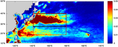
Fig. 1 Long-term mean (2006–2009) eddy kinetic energy (units: m² s⁻²) in the North Pacific. The black rectangle area represents the KE region. The WRF model domain is represented by the red dashed rectangle area.

The remainder of the paper is organised as follows. We introduce the datasets and methods in Section 2. Atmospheric responses to the oceanic eddies in all four seasons based on the observations are discussed in Section 3. Atmospheric responses based on the Climate Forecast System Reanalysis (CFSR) data of the National Centers for Environmental Prediction (NCEP) are presented in Section 4. The Weather Research and Forecast (WRF) model is employed to investigate the seasonal variations in atmospheric responses to idealised eddies in Section 5. Summary and discussion are given in Section 6.

2. Data and methods

2.1. Data

NOAA’s National Climate Data Center (NOAA/NCDC) sea surface winds on a 0.25°×0.25° grid are used for the period of 2006–2009. The wind speeds were generated by blending observations from multiple satellites (up to six satellites since June 2002) to reduce subsampling aliases and random errors (Zhang et al., 2006).

We use the 3-day-averaged daily SST, column-integrated cloud liquid water content and rain rate with a horizontal resolution of 0.25° longitude by 0.25° latitude for the period of 2006–2009 from Tropical Rainfall Measuring Mission's (TRMM) Microwave Imager (TMI; Wentz et al., 2000). Daily latent and sensible heat fluxes on a 0.25°×0.25° grid are obtained from the Japanese Ocean Flux Data sets with Use of Remote Sensing Observations (J-OFURO; Kubota et al., 2002) version 2 for the period of 2006–2007. According to the comparison results of J-OFURO, in situ observations from the Kuroshio Extension Observatory (KEO) and JAMSTEC KEO (JKEO) surface moorings, and global air–sea heat flux products from numerical weather prediction, J-OFURO2 air–sea heat fluxes are best data set for air–sea interaction study over the Kuroshio Extension region (Tomita et al., 2010).

The CFSR data include all available conventional and satellite observations and provide the best estimate of the states of atmosphere–ocean–land surface–sea ice system (Saha et al., 2010). Xue et al. (2011) showed that the surface heat fluxes and wind stress from the CFSR generally agree with observations, and they are better than those in the NCEP/NCAR reanalysis (R1) and NCEP/DOE reanalysis (R2). We use the 6-hourly SST, surface winds at 10 m, latent and sensible heat fluxes and MABL height at the resolution of 0.313° latitude by 0.312° longitude during the period of 2006–2009. CFSR 6-hourly three-dimensional winds and air temperatures at isobaric levels on a 0.5°×0.5° grid are also used.

2.2. Methods

2.2.1. Eddy identification.

Nencioli et al. (2010) developed an eddy detection scheme based on velocity geometry and applied this scheme to output from a numerical model; Dong et al. (2011) and Liu et al. (2012) applied it to thermal-wind velocity field and geostrophic velocity anomalies derived from sea surface height anomaly (SSHA), respectively. Ma et al. (2015) used the eddy dataset obtained from Dong et al. (2011) to investigate the atmospheric responses to oceanic eddies in the KE region. Refer to Dong et al. (2011) and Ma et al. (2015) for the specific steps of eddy detection.

2.2.2. Composite analysis.

To examine the characteristics of atmospheric responses in different seasons, we present the composites of SST and other variables for the identified cold and warm eddies. Eight-longitude-degree moving average is removed from all the variables. A box of 4°×4° relative to each eddy centre is chosen as the composite area. All variables are rotated according to the large-scale wind direction (defined as the area–mean wind direction) to better show the atmospheric responses. The large-scale mean wind direction is used as the new x-axis after the rotation. Eddies with SST anomaly less than −0.1 °C and larger than 0.1 °C at the eddy centre are chosen for further analysis. 17,200 cold eddies and 17,700 warm eddies in the KE region (140°–180°E, 28°–40°N) from 2006 to 2009 are selected. The cold eddy numbers in winter (December–February, or DJF), spring (March–May, or MAM), summer (June–August, or JJA) and autumn (September–November, or SON) are 4632, 4890, 3618 and 4138, respectively; the warm eddy numbers are 4716, 4343, 3856 and 4874, respectively.

2.2.3. Linear fitting, F test, t test and bandpass filter.

Linear regressions are made to SST-q (another variable) anomaly scattergrams to obtain quantitative estimates of the atmospheric responses to oceanic eddies. The significance of the linear fitting is assessed using the F test. We also use t test to determine the significance of the composite results.

The vertical transport of synoptic-scale transient zonal momentum is calculated. and represent synoptic-scale transient zonal and vertical winds, respectively, which are obtained using the 31-point bandpass filter (Sun and Zhang, 1992). More details about the 31-point bandpass filter can be found in Ma et al. (2015).

2.2.4. Weather Research and Forecast (WRF) model.

To examine the seasonal variations in atmospheric responses to the oceanic eddies in the KE region, the WRF model (version 3.5; Skamarock et al., 2008) is also employed, which is a fully compressible and non-hydrostatic model.

3. Atmospheric responses in the observations

3.1. Surface wind speed

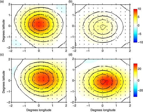
Figures 2a and b present the composites of SST anomalies and wind speed anomalies for the warm eddies in winter and summer, respectively. The composites show that warmer SST anomalies accelerate surface winds, with some phase differences between positive wind speed anomalies and SST anomalies. The maximum SST anomalies and wind speed anomalies in winter are about 0.8 °C and 0.3 m s⁻¹, respectively. The warm eddies weaken remarkably in summer, with maximum SST anomalies of 0.5 °C and maximum surface wind speed anomalies only about 0.15 m s⁻¹. In spring (not shown), the maximum SST anomalies and wind speed anomalies are about 0.7 °C and 0.3 m s⁻¹, respectively. The eddies in autumn are stronger than those in summer, but still much weaker than those in cold seasons (winter and spring). The relationships between wind speed anomalies and SST anomalies are quantified based on the linear fitting with wind speed anomalies as a function of SST anomalies. The linear fits yield slopes of 0.307, 0.319, 0.209 and 0.252 m s⁻¹ °C⁻¹ in winter, spring, summer and autumn, respectively (all significant at the 0.05 level in the F test), which clearly shows that the surface wind speed responses in the cold seasons are much stronger than those in the warm seasons (summer and autumn). The slopes of straight-line fits to SST anomalies for all the variables are summarised in Table 1.

Fig. 2 Top panels: Composites of TMI SST anomalies (contours at the interval of 0.1 °C) and observational surface wind speed anomalies (shadings; units: m s⁻¹). Bottom panels: CFSR reanalysis SST anomalies (contours at the interval of 0.1 °C) and CFSR surface wind speed anomalies (shadings; units: m s⁻¹) for the warm eddies in winter (a, c) and summer (b, d). Areas with dots pass a two-tailed t test at the 0.05 level.

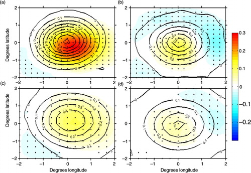
Table 1. Slopes of linear fits of some variables vs. SST anomalies

	Cold eddy				Warm eddy
	Winter	Spring	Summer	Autumn	Winter	Spring	Summer	Autumn
Surface wind speed (ms^−1 °C^−1)	0.321	0.324	0.209	0.223	0.307	0.319	0.209	0.252
CFSR surface wind speed (ms^−1 °C^−1)	0.223	0.205	0.132	0.185	0.220	0.203	0.119	0.179
Sensible heat flux (W m^−2 °C^−1)	15.257	10.638	5.897	9.449	15.693	10.396	5.823	9.163
CFSR sensible heat flux (W m^−2 °C^−1)	16.668	10.794	5.625	9.687	16.738	11.082	5.550	9.630
Latent heat flux (W m^−2 °C^−1)	23.146	17.656	13.592	22.777	22.371	15.361	13.761	21.767
CFSR latent heat flux (W m^−2 °C^−1)	41.534	29.683	26.300	40.881	41.938	29.824	27.057	41.059
CFSR MABL height (m °C^−1)	47.734	52.878	56.138	62.756	50.787	51.668	66.974	61.048

For the cold eddies, the wind speed composites demonstrate that surface winds decelerate over the eddies with some phase discrepancies (not shown). The eddies in summer are much weaker than those in winter in terms of SST anomalies due to the stronger stratification in the upper ocean in summer. The slopes of linear fitting in all four seasons show that surface wind speed responses are stronger in the cold seasons than in the warm seasons for the cold eddies, which is the same as the case for the warm eddies.

3.2. Heat fluxes

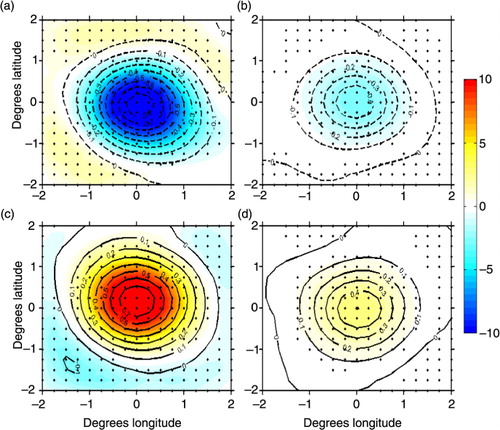
Figures 3a and b show the composites of sensible heat flux (from J-OFURO) anomalies over the cold eddies in winter and summer, respectively. Note that the upward flux is defined to be positive. Negative sensible heat flux anomalies are found over the cold eddies in both seasons. The minimum sensible heat flux anomaly is −2 W m⁻² in summer, −10 W m⁻² in winter. In spring and autumn (not shown), the minima are about −6 and −4 W m⁻², respectively. Linear fits of sensible heat flux anomalies versus SST anomalies yield slopes of 15.257, 10.638, 5.897 and 9.449 W m⁻² °C⁻¹ in winter, spring, summer and autumn, respectively (all significant at the 0.05 level in the F test). It indicates that the cold eddies reduce the sensible heat flux more efficiently in the cold seasons than in the warm ones. The composites and linear fitting of latent heat flux anomalies to SST anomalies show that the responses of latent heat flux are the weakest in summer. Different from the sensible heat flux, the latent heat flux in autumn responds more strongly than in spring, with the regression slopes of 23.146, 17.656, 13.592 and 22.777 for the cold eddies in winter, spring, summer and autumn, respectively (all significant at the 0.05 level in the F test). The seasonal variations in sensible heat flux for the warm eddies (Figs. 3c and d) and in latent heat flux for the warm eddies (not shown) are consistent with those for the cold eddies.

Fig. 3 Composites of TMI SST anomalies (contours at the interval of 0.1 °C) and J-OFURO sensible heat flux anomalies (shadings; units: Wm⁻²) for the cold (a, b) and warm (c, d) eddies in winter (a, c) and summer (b, d). Areas with dots pass a two-tailed t test at the 0.05 level.

The above results indicate that there exist significant seasonal variations in the responses of surface wind speed and heat fluxes to oceanic eddies in the KE region. In general, the responses are stronger in the cold seasons than in the warm seasons, and the response is the strongest in winter and the weakest in summer.

3.3. Cloud liquid water and rain rate

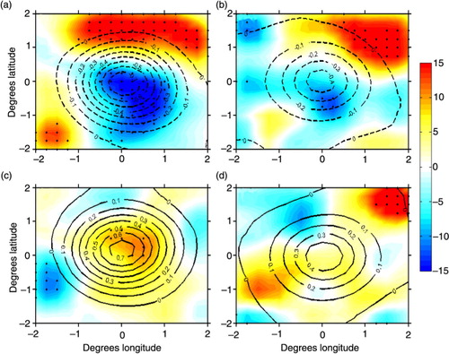
The composites of cloud liquid water anomalies also display seasonally dependent characteristics, shown in Fig. 4. The cloud liquid water in winter is in much more deficit (surplus) than in summer over the cold (warm) eddies. Figure 5 presents the composites of rain rate anomalies, which shows that rain rate anomalies in summer are of smaller magnitude and more scattering than in winter over both cold and warm eddies.

Fig. 4 Composites of TMI SST anomalies (contours at the interval of 0.1 °C) and cloud liquid water anomalies (shadings; units: 1×10⁻³ mm) for the cold (a, b) and warm (c, d) eddies in winter (a, c) and summer (b, d). Areas with dots pass a two-tailed t test at the 0.05 level.

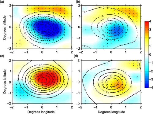
Fig. 5 Composites of TMI SST (contours at the interval of 0.1 °C) and rain rate anomalies (shadings; units: 1×10⁻³ mm h⁻¹) for the cold (a, b) and warm (c, d) eddies in winter (a, c) and summer (b, d). Areas with dots pass a two-tailed t test at the 0.05 level.

4. Atmospheric responses in the CFSR data

4.1. Surface wind speed and heat fluxes

The composites of SST anomalies and surface wind speed anomalies for the warm eddies based on the CFSR reanalysis data are shown in Figs. 2c and d. The positive correlation between SST anomalies and surface wind speed anomalies is quite similar to that based on the satellite observations. Although the warm eddies are relatively weaker with the maximum SST anomaly of about 0.4 °C in comparison with the satellite result, they are the strongest in winter and the weakest in summer, consistent with the seasonal variation characteristics of the observational results. The regression slopes of wind speed anomalies to SST anomalies are 0.220, 0.203, 0.119 and 0.179 m s⁻¹ °C⁻¹ in winter, spring, summer and autumn, respectively (all significant at the 0.05 level in the F test). In spite of the much smaller magnitudes than those in the satellite observations, surface wind speeds are more responsive in the cold seasons than in the warm seasons in the CFSR dataset, as in the observations. The results for the cold eddies are similar to those for the warm eddies (not shown).

Consistent with the results based on the J-OFURO data, the CFSR data also shows that positive sensible heat flux anomalies occur over the warm eddies (Figs. 6a and b). The latent heat flux result using the CFSR data shows weaker eddies than those in the observations, but larger latent heat flux anomalies than in the observations, which is clearly seen from the slopes of linear fitting of latent heat flux anomalies versus SST anomalies. The slopes for the cold eddies are 41.534, 29.6827, 26.300 and 40.881 W m⁻² °C⁻¹ in winter, spring, summer and autumn, respectively (all significant at the 0.05 level in the F test), prominently larger than those based on the J-OFURO data, which suggests that the difference between air humidity and saturated humidity at SST is much larger than the J-OFURO data. Albeit with this difference, the seasonal variation in the response is consistent with that based on the J-OFURO data.

Fig. 6 Top panels: Composites of CFSR reanalysis SST anomalies (contours at the interval of 0.1 °C) and CFSR sensible heat flux anomalies (shadings; units: Wm⁻²). Bottom panels: Same contours as in the top panels and MABL height anomalies (shadings; units: m) for the warm eddies in winter (a, c) and summer (b, d). Areas with dots pass a two-tailed t test at the 0.05 level.

4.2. MABL height

O'Neill et al. (2005) speculated that the seasonal variations in wind stress curl and divergence in response to SST anomalies are associated with MABL height differences. Figures 6c and d present the composites of CFSR MABL height anomalies over the warm eddies in winter and summer, respectively. The positive correlations between SST and MABL height anomalies are robust in all four seasons (figures for spring and autumn are not shown). Linear fits yield slopes of 50.787, 51.668, 66.974 and 61.048 m °C⁻¹ in winter, spring, summer and autumn, respectively (all significant at the 0.05 level in the F test), which indicates that MABL height responds more strongly in the warm seasons than in the cold seasons. MABL height is defined as the height where the bulk Richardson number reaches a critical value, typically 0.25 (Gryning and Batchvarova, 2002). The bulk Richardson number is closely related to the vertical gradient of virtual potential temperature. Due to the wintertime intense mixing in the MABL (as seen in Section 4.4), the eddy-induced change in vertical gradient of virtual potential temperature is very small. In contrast, the change in summer is larger, as a result of weak MABL mixing. This may contribute to the seasonal variation characteristics of MABL height response.

4.3. MABL stability

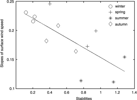
Figure 7 presents the scatterplot of stability (defined as the difference between virtual potential temperature at 950 hPa and that at 1000 hPa) and slopes of wind speed anomalies versus SST anomalies in the 12 calendar months. The slopes are negatively correlated to the stability, indicating that a relatively unstable boundary layer can induce stronger responses of wind speed to the oceanic eddies. In addition, it can be readily seen that the boundary layer is more unstable in winter than in summer. Therefore, the seasonal variation in surface wind speed responses may be attributed to the differences in background atmospheric static stability in different seasons. O'Neill et al. (2005) suggested that the seasonal dependence of wind stress curl and divergence responses to SST anomalies can be explained by the annual cycle of large-scale lower tropospheric stability over the ARC region.

Fig. 7 Scatterplot of static stabilities and slopes of surface wind speed anomalies versus SST anomalies in the 12 calendar months.

Two primary mechanisms have been put forward to explain the mesoscale SST–surface wind relationship. The first mechanism is the sea level pressure (SLP) mechanism proposed by Lindzen and Nigam (1987), which indicates that SLP tends to fall (rise) over warm (cold) SST anomalies, yielding a wind acceleration (deceleration) upstream (downstream) of warm SST anomalies (Small et al. 2003). The second mechanism is referred to as the vertical momentum mixing mechanism, which suggests that the relatively unstable (stable) MABL induces stronger (weaker) surface wind by strengthening (weakening) vertical momentum mixing above warmer (colder) water (Wallace et al., 1989; O'Neill et al., 2003; Chelton et al., 2004). Since vertical mixing is closely related to stability, the seasonal variation in vertical momentum mixing makes a great contribution to the seasonal variation in wind speed response. This indicates that the vertical momentum mixing mechanism plays a leading role in the wind speed response to the oceanic eddies in the KE region.

4.4. Vertical transport of transient zonal momentum and wind velocity

Recent studies (Ma et al., 2014, 2015) demonstrated that atmospheric responses can extend into free troposphere over oceanic eddies. The above analyses show that the CFSR data can well capture the seasonal variations in the atmospheric responses to the oceanic eddies in the MABL of the KE region. Next, the CFSR data are used to investigate atmospheric responses beyond the MABL.

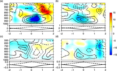
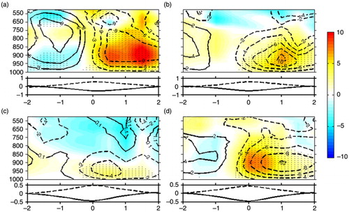
Figures 8a–d show the longitude-height cross-sections of composite along the eddy centre's latitude in all four seasons. In winter (Fig. 8a), negative anomalies occur over the cold eddy centre from the sea surface to the 800-hPa level. A nearly opposite pattern holds for the warm eddies in winter (Fig. 8a; contours). The significant differences between cold and warm eddies extend to about 850 hPa. Positive values of represent downward transport of transient zonal momentum, as vertical velocities at isobaric levels (ω) are used, inducing wind acceleration, while negative values represent weakening of downward momentum transport, causing wind deceleration. In spring (Fig. 8b), the negative anomalies over the cold eddy centre can also extend to the 800-hPa level, but with less intensity. For the warm eddies (Fig. 8b; contours), positive anomalies appear over the eddy centre, but the extension height is lower than that for the cold eddies. The negative (positive) anomalies of over the cold (warm) eddies in autumn (Fig. 8d) are much weaker, and the differences between cold and warm eddies are significant only below 950 hPa. In summer (Fig. 8c), the differences of anomalies between cold and warm eddies hardly pass the significance test.

Fig. 8 Longitude-height cross-sections of the composite vertical transport anomalies of transient zonal momentum (units: 1×10⁻³ Pa m s⁻²) along the cold (shown in shadings) and warm (shown in contours) eddy centre's latitude in winter (a; contour interval of 5×10⁻³ Pa m s⁻²), spring (b; contour interval of 3×10⁻³ Pa m s⁻²), summer (c; contour interval of 2×10^-3 Pa m s⁻²) and autumn (d; contour interval of 3×10⁻³ Pa m s⁻²). Areas with dots pass a two-tailed t test at the 0.05 level. Composites of SST anomalies along the cold (warm) eddy centre's latitude are shown in solid (dashed) lines below each cross-section.

Similar seasonal variation features are shown by the longitude-height cross-sections of the composite wind velocity along the eddy centre's latitude in all four seasons (Figs. 9a–d). Over the cold eddies, the minimum wind speed anomalies appear near the sea surface and the negative anomalies penetrate to the 900-hPa level, tilting downstream with increasing altitude in winter. The result for the warm eddies exhibit nearly opposite patterns to that for the cold eddies (Fig. 9a; contours). Significant differences between cold and warm eddies extend above 975 hPa (Fig. 9a). In spring (Fig. 9b), the significant differences between cold and warm eddies only appear below 975 hPa. The negative (positive) anomalies in summer only occur near the surface, while the maximum (minimum) anomalies are located between 975 and 950 hPa over cold (warm) eddies (Fig. 9c). The wind speed anomaly pattern in autumn is similar to that in spring, but with less intensity. The significant differences between cold and warm eddies appear between 975 and 925 hPa (Fig. 9d). Perlin et al. (2014) revealed that wind speed response to local SST anomalies in winter decreases rapidly, approaching zero at 150–300 m, and there is virtually no sensitivity of the wind speed to SST anomalies above 600–800 m, which is similar to what we found in winter. Ma et al. (2015) speculated that the difference between their multi-year mean wind speed anomalies and the wintertime results by Perlin et al. (2014) may be a result of seasonal variation. Our results support their speculation.

Fig. 9 Same as in Fig. 8, except for the composite wind speed anomalies (units: m s⁻¹).

It should be pointed out that the maximum SST anomalies in winter and summer are about 0.8 and 0.5 °C, respectively; however, and wind speed responses in summer are much weaker than those in winter. From that, we can infer that the oceanic eddies can induce stronger imprints on the overlying atmosphere in winter than in summer, provided that the eddies have the same intensity.

4.5. Vertical velocity

Figure 10 presents the vertical cross-sections of vertical velocity along the cold eddy centre's latitude in all four seasons. The vertical velocity also exhibits seasonally dependent structures. Figure 10a shows that anomalous subsidence appears over the cold eddy centre in winter, with maximum anomalies shifted downstream. This is probably related to the wind divergence, which results from the wind deceleration over the cold eddy (Xu et al., 2011; Ma et al., 2015). Note that the vertical velocity anomalies can extend to 750-hPa and even higher level. In spring (Fig. 10b), the anomaly pattern is similar to that in winter, but with much weaker anomalies. In summer (Fig. 10c), the anomalous subsidence occurs above the eddy centre and downstream, with positive anomalies extending to the 900-hPa level. In autumn (Fig. 10d), anomalous subsidence appears over the eddy centre and reaches 750 hPa. For the warm eddies (Fig. 10; contours), a nearly opposite pattern appears to that of the cold cases in each season. To sum up, the impact of oceanic eddies on vertical velocity is confined near the sea surface in summer, while the eddies exert significant impacts on vertical velocity at higher levels in winter. Similar to the conclusion drawn in Section 4.4, the oceanic eddies can induce stronger imprints on vertical velocity in winter than in summer, provided that the eddies have the same intensity.

Fig. 10 Same as in Fig. 8, except for the composite vertical velocity anomalies (shadings; units: 1×10⁻³ Pa s⁻¹).

5. Modelling results

5.1. Experimental design

In this section, the modelling results from WRF model are used to further investigate the seasonal variations in atmospheric responses to the oceanic eddies in the KE region. The model domain is 140°–180°E, 20°–40°N (refer to Fig. 1). The model uses a horizontal resolution of 30 km by 30 km and has 28 sigma levels in the vertical. The parameterisation schemes used in the model and their corresponding references are listed in Table 2. The initial and lateral boundary conditions are obtained from the NCEP FNL (Final) Operational Global Analysis data on 1° by 1° grids prepared operationally every 6 hours. This is the product from the Global Data Assimilation System (GDAS) and NCEP Global Forecast System (GFS) model. Over the ocean, the daily Real-Time Global SST analysis (RTG) SSTs (www.polar.ncep.noaa.gov/sst/rtg_low_res/) are employed as the lower boundary condition.

Table 2. List of physics parameterisation schemes used in the WRF model

Microphysics	WSM 3-class simple ice scheme (Dudhia et al., 2008)
Longwave radiation	RREM scheme (Mlawer et al., 1997)
Shortwave radiation	Dudhia scheme (Dudhia, 1989)
Surface layer	Monin–Obukhov (Janjic Eta) scheme (Janjic, 2002)
Land surface	Noah scheme (Chen and Dudhia, 2001)
Boundary layer	Mellor–Yamada–Janjic scheme (Janjic, 1994)
Cumulus convection	Kain–Fritsh scheme (Kain and Fritsch, 1993; Kain, 2004)

We perform two sets of experiments, one is the control (CTL) run and the other is the warm eddy (WE) run (The conclusions would be similar if we use a cold eddy instead). Both sets of experiments comprise the winter and summer cases. Each set of experiments consists of an ensemble offive simulations with 48-hour integrations which are initialised at 00 UTC, 15 February, 18 February, 20 February, 23 February, 26 February (2008) for the winter cases, and 15 June, 18 June, 20 June, 23 June, 26 June (2008) for the summer cases. These dates are chosen randomly. For all the experiments, the CTL runs are forced by zonal mean SST over the model domain, and the WE runs are the same as the CTL run except that the SST is superimposed with a warm eddy with a diameter of about 3° and the maximum SST anomaly of 2.0 °C in the KE region (contours in Figs. 11a–d). It is worth noting that, in all the cases, the initial fields and subsequent 6-hourly inputs including SLP, winds, temperature, geopotential height and relative humidity are zonally averaged along the longitudes of the model domain to isolate the warm eddy's effects on the overlying atmosphere.

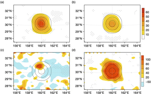
Fig. 11 SST differences (a–d; contours; units: °C), upward heat flux differences (a, b; shadings; units: W m⁻²) and MABL height differences (c, d; shadings; units: m) between the WE and CTL runs in winter (a, c) and summer (b, d). Areas with dots pass a two-tailed t test at the 0.05 level.

We discuss the ensemble mean 36-hour averages from the 12th to the 48th hours, based on 3-hour averages of model outputs. The variables are also rotated according to the background wind for the sake of comparison with the observations (the easterlies prevail in the summer case).

5.2. Results

The SST differences between the WE and CTL runs are shown in Fig. 11, which are characterised by a circle with a diameter of about 3°. Latent heat flux differences between the WE and CTL runs are shown as shadings. Positive heat flux differences occur over the warm eddies in both winter and summer cases. In winter, the maximum heat flux difference is more than 60 W m⁻², while the maximum in summer is only about 40 W m⁻². The characteristics of seasonal difference are consistent with the observations. With regard to MABL height (Figs. 11c–d), its differences in summer are better organised over the warm eddy and larger than those in winter, sharing consistency with the observational results.

Figures 12a and b present the longitude-height cross-sections of wind speed differences between the WE and CTL runs along the eddy centre's latitude in winter and summer, respectively. In winter (Fig. 12a), the wind acceleration over the warm eddy extends near 700 m (σ≅0.91). In summer (Fig. 12b), an increase in wind speed also occurs over the warm eddy, but the positive differences are confined near the surface below 300 m (σ≅0.96). In addition, the magnitude of wind speed response to the warm eddy in winter is larger than that in summer. It should be pointed out that the negative differences over the warm eddy in the summer case are not significantly different from the marked negative anomalies over the warm eddies, shown in Fig. 9 with contours.

Fig. 12 Longitude-height cross-sections of wind speed differences (shadings; units: ms⁻¹) and turbulent kinetic energy differences (contours; units: m² s⁻²) between the WE and CTL runs along the eddy centre's latitude in winter (a; contour interval of 0.02 m² s⁻²) and summer (b; contour interval of 0.005 m² s⁻²). The vertical coordinate shows the model sigma levels. Areas with dots pass a two-tailed t test at the 0.05 level. Composite of SST differences along the eddy centre's latitude is shown below each cross-section.

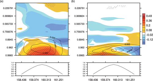
The turbulent kinetic energy (TKE) exhibits similar seasonal variation. Figure 12 shows the longitude-height cross-sections of TKE differences using contours. It can be readily seen that an increase in TKE appears over the warm eddy in winter, and the increase extends to about 1000 m (σ≅0.88) with a maximum of 0.06 m² s⁻². By contrast, in summer, only a weak response in TKE appears below 400 m (σ≅0.95) with a maximum of 0.02 m² s⁻², much weaker than that in winter.

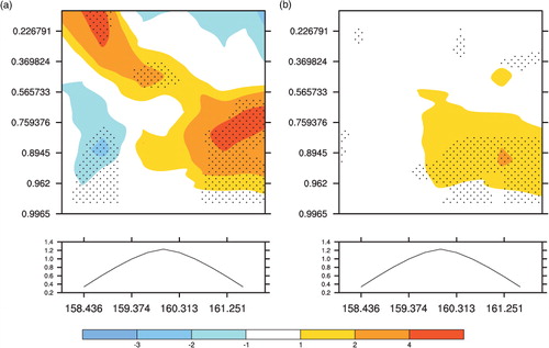
The vertical velocity differences between the WE and CTL runs are also examined, as shown in Fig. 13. The vertical velocity displays similar seasonally dependent structures with the maximum differences of 4×10⁻³and 2×10⁻³m s⁻¹and maximum height extensions of 5000 (σ≅0.5) and 2000 (σ≅0.75) m in winter and summer, respectively, though the upward motion appears over the warm eddy and downstream in both winter and summer.

Fig. 13 Same as in Fig. 12, except for vertical velocity differences (shadings; units: 1×10⁻³ m s⁻¹).

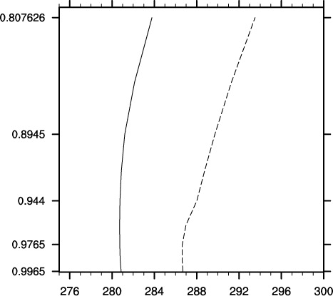
The profiles of virtual potential temperature averaged over the model domain (Fig. 14) indicate that the atmosphere boundary layer is neutral and even unstable below 800 m (σ≅0.9) in winter. However, the MABL is quite stable in summer, with a shallow neutral layer near the sea surface. The vertical gradient of virtual potential temperature below about 1400 m (σ≅0.807) in winter is much smaller than that in summer. The seasonal difference is in agreement with the result based on the CFSR data, suggesting that the background MABL static stability acts as a significant role in seasonal variation of atmospheric responses to oceanic eddies.

Fig. 14 Profiles of virtual potential temperature (units: K) averaged over the model domain in winter (solid line) and summer (dashed line) in CTL runs. The vertical coordinate refers to the model sigma levels.

6. Summary and discussion

In this study, seasonal variations in atmospheric responses to the oceanic eddies in the KE region in all four seasons are investigated using methods such as composite, moving average and bandpass filter. The seasonal variations show much stronger surface wind speed and heat flux responses in the cold seasons than in the warm seasons. Specifically, the cold (warm) eddies decrease (increase) the sensible heat flux more efficiently in the cold seasons than in the warm seasons; the latent heat fluxes are most responsive in winter and least responsive in summer, and more responsive in autumn than in spring; cloud liquid water and rain rate are both in more deficit (surplus) in winter than in summer over the cold (warm) eddies.

The CFSR data can well reproduce the seasonal variations in atmospheric responses to the KE eddies in the MABL. Although the responses are much weaker than those in the satellite observations, surface wind speeds are more responsive in the cold seasons than in the warm seasons in the CFSR data. In addition, although weaker eddies induce larger latent heat flux anomalies in the CFSR reanalysis data compared to the J-OFURO results, the seasonal variations in latent heat flux response are similar for the two datasets. In particular, the MABL height responds more strongly in the warm seasons than in the cold seasons.

The CFSR data also show significant seasonal variations in tropospheric atmospheric responses. Negative (positive) anomalies of vertical transport of transient zonal momentum appear over the cold (warm) eddy centre, while the anomalies in summer and autumn are quite weak and diffused. With regard to the wind speed, its anomalies over the eddies can penetrate to the 900-hPa level in winter; in summer, the anomalies with the same sign as the SST anomalies only occur near the surface, but the anomalies with the opposite sign to the SST anomalies appeared between 975 and 950 hPa. Additionally, the impact of oceanic eddies on vertical velocity is confined below 900 hPa in summer, while significant eddy impacts on the vertical velocity extend to 800 hPa in winter.

The WRF model is used to investigate the seasonal variations. Comparison of the winter and summer experiments suggests that the characteristics of seasonal variations in responses of wind speed, heat flux, MABL height, vertical velocity, etc. are in agreement with the observational results.

Results from both the CFSR data and WRF simulations indicate that the MABL is relatively unstable in winter, and stable in summer, and that the seasonal variations in atmospheric responses can be attributed to the seasonal variation in background atmospheric static stability. In addition, as vertical mixing is closely related to the stability, the stronger vertical momentum mixing in winter than in summer contributes greatly to the stronger wind speed response in winter than in summer. This indicates that the vertical momentum mixing mechanism plays a significant role in the wind speed responses to the oceanic eddies over the KE region.

It is noteworthy that atmospheric responses to oceanic eddies can feed back to the ocean by affecting Ekman pumping through wind stress curl changes. Frenger et al. (2013) also pointed out that changes in wind speed and cloud fraction could induce eddy dissipation, constituting a negative feedback, while rainfall changes could intensify eddies. The WRF results in the present study only showed part of the complex interactions involving the coupled ocean–atmosphere system. Therefore, it is necessary to use a coupled ocean–atmosphere model to investigate these interaction processes and shed light on the seasonal variations.

7. Acknowledgements

The TMI data are sponsored by the NASA Earth Science MEaSUREs DISCOVER Project, produced by the Remote Sensing Systems, and available at www.remss.com. This work is jointly supported by the Ministry of Science and Technology of China (National Basic Research Program of China under grants 2012CB955602 and 2014CB745000), the National Natural Science Foundation of China (41490643, 41275094 and 41476022), the “Qinglan Project” of Jiangsu Province of China, the Project funded by the Priority Academic Program Development of Jiangsu Higher Education Institutions (PAPD), the Startup Foundation for Introducing Talent of Nanjing University of Information Science and Technology (2013r121 and 2014r072), the Program for Innovation Research and Entrepreneurship Team in Jiangsu Province, and the National Programme on Global Change and Air-Sea Interaction (No. GASI-03-IPOVAI-05). This work, part of Jing Ma's PhD Training Program in Scripps Institute of Oceanography, is also sponsored by China Scholarship Council. We thank Yu Liu for providing the eddy dataset. We are also grateful to two anonymous reviewers for their comments and suggestions that helped improve the manuscript.

References

- Bourras D., Reverdin G., Giordani H., Caniaux G. Response of the atmospheric boundary layer to a mesoscale oceanic eddy in the northeast Atlantic. J. Geophys. Res. Atmos. 2004; 109: 1–19. DOI: http://dx.doi.org/10.1029/2004JD004799.
- Chelton D. B. , Schlax M. G. , Freilich M. H. , Milliff R. F . Satellite measurements reveal persistent small-scale features in ocean winds. Science. 2004; 303: 978–983.
- Chelton D. B., Schlax M. G., Samelson R. M., de Szoeke R. A. Global observations of large oceanic eddies. Geophys. Res. Lett. 2007; 34 L15606, DOI: http://dx.doi.org/10.1029/2007GL030812.
- Chen F. , Dudhia J . Coupling an advanced land surface-hydrology model with the Penn State-NCAR MM5 modeling system. Part II: Preliminary model validation. Mon. Weather Rev. 2001; 129: 587–604.
- Dong C. M. , Nencioli F. , Liu Y. , McWilliams J. C . An automated approach to detect oceanic eddies from satellite remotely sensed sea surface temperature data. IEEE Geosci. Remote Sen. Lett. 2011; 8: 1055–1059.
- Dudhia J . Numerical study of convection observed during the winter monsoon experiment using a mesoscale two-dimensional model. J. Atmos. Sci. 1989; 46: 3077–3107.
- Dudhia J. , Hong S. Y. , Kim K. S . A new method for representing mixed-phase particle fall speeds in bulk microphysics parameterizations. J. Met. Soc. Japan. 2008; 86A: 33–44.
- Frenger I. , Gruber N. , Knutti R. , Munnich M . Imprint of Southern Ocean eddies on winds, clouds and rainfall. Nat. Geosci. 2013; 6: 608–612.
- Gryning S. E. , Batchvarova E . Marine boundary-layer height estimated from the HIRLAM model. Boreal Environment Research. 2002; 7: 229–234.
- Hashizume H. , Xie S. P. , Liu W. T. , Takeuchi K . Local and remote atmospheric response to tropical instability waves: A global view from space. Journal of Geophysical Research. 2001; 106(D10): 10173–10185.
- Janjic Z. I . The Step-Mountain Eta Coordinate Model – further developments of the convection, viscous sublayer, and turbulence closure schemes. Mon. Weather Rev. 1994; 122: 927–945.
- Janjic Z. I . Nonsingular Implementation of the Mellor-Yamada Level 2.5 Scheme in the NCEP Meso Model. 2002; 61. NCEP office note, 437.
- Kain J.S. , Fritsch J.M . Convective parameterization for mesoscale models: The Kain-Fritsch scheme. In The representation of cumulus convection in numerical models . 1993; 165–170. American Meteorological Society.
- Kain J. S . The Kain-Fritsch convective parameterization: an update. J. Appl. Meteorol. 2004; 43: 170–181.
- Kubota M. , Tomita H . Present state of the J-OFURO air-sea interaction data product. Flux News. 2007; 4: 13–15.
- Lindzen R. S. , Nigam S . On the role of sea-surface temperature-gradients in forcing low-level winds and convergence in the tropics. J. Atmos. Sci. 1987; 44: 2418–2436.
- Liu T. W. , Xie X. , Polito P. S. , Xie S.-P. , Hashizume H . Atmospheric manifestation of tropical instability wave observed by QuikSCAT and tropical rain measuring mission. Geophys. Res. Lett. 2000; 27: 2545–2548.
- Liu W. T. , Xie X. , Niiler P. P . Ocean-Atmosphere Interaction over Agulhas Extension Meanders. Journal of Climate. 2007; 20(23): 5784–5797.
- Liu Y. , Dong C. , Guan Y. , Chen D. , McWilliams J. , Nencioli F . Eddy analysis in the subtropical zonal band of the North Pacific Ocean. Deep Sea Res. I. Oceanogr. Res. Papers. 2012; 68: 54–67.
- Ma J., Xu H. M., Dong, C. M. Atmospheric response to mesoscale oceanic eddies over the Kuroshio Extension: case analyses of warm and cold eddy in winter. Chin. J. Atmos. Sci. 2014; 38(3): 438–452. DOI: http://dx.doi.org/10.3878/j.issn.1006-9895.2013.13151. (in Chinese with English abstract).
- Ma J. , Xu H. M. , Dong C. M. , Lin P. F. , Liu Y . Atmospheric responses to oceanic eddies in the Kuroshio Extension region. J. Geophys. Res. Atmos. 2015; 120: 6313–6330.
- Minobe S. , Kuwano-Yoshida A. , Komori N. , Xie S. P. , Small R. J . Influence of the Gulf Stream on the troposphere. Nature. 2008; 452(7184): 206–209.
- Minobe S. , Miyashita M. , Kuwano-Yoshida A. , Tokinaga H. P. , Xie S.-P . Atmospheric response to the Gulf Stream: Seasonal variations. Journal of Climate. 2010; 23(13): 3699–3719.
- Mlawer E. J. , Taubman S. J. , Brown P. D. , Iacono M. J. , Clough S. A . Radiative transfer for inhomogeneous atmospheres: RRTM, a validated correlated-k model for the longwave. J. Geophys. Res. Atmos. 1997; 102: 16663–16682.
- Namias J. , Cayan D. R . Large-scale air-sea interactions and short-period climatic fluctuations. Science. 1981; 214(4523): 869–876.
- Nencioli F. , Dong C. M. , Dickey T. , Washburn L. , McWilliams J. C . A vector geometry-based eddy detection algorithm and its application to a high-resolution numerical model product and high-frequency radar surface velocities in the Southern California Bight. J. Atmos. Ocean. Technol. 2010; 27: 564–579.
- Nonaka M. , Xie S.-P . Covariations of sea surface temperature and wind over the Kuroshio and its extension: evidence for ocean-to-atmosphere feedback. J. Clim. 2003; 16: 1404–1413.
- O'Neill L. W. , Chelton D. B. , Esbensen S. K . Observations of SST-induced perturbations of the wind stress field over the Southern Ocean on seasonal timescales. J. Clim. 2003; 16: 2340–2354.
- O'Neill L. W. , Chelton D. B. , Esbensen S. K . High-resolution satellite measurements of the atmospheric boundary layer response to SST variations along the Agulhas Return Current. J. Clim. 2005; 18: 2706–2723.
- Perlin N. , de Szoeke S. P. , Chelton D. B. , Samelson R. M. , Skyllingstad E. D. , co-authors . Modeling the atmospheric boundary layer wind response to mesoscale sea surface temperature perturbations. Mon. Weather Rev. 2014; 142: 4284–4307.
- Qiu B. , Chen S. M . Interannual variability of the North Pacific subtropical countercurrent and its associated mesoscale eddy field. J. Phys. Oceanogr. 2010; 40: 213–225.
- Saha S. , Moorthi S. , Pan H. L. , Wu X. R. , Wang J. D. , co-authors . The NCEP climate forecast system reanalysis. Bull. Am. Meteorol. Soc. 2010; 91: 1015–1057.
- Skamarock W. C. , Klemp J. B. , Dudhia J. , Gill D. O. , Barker D. , co-authors . A Description of the Advanced Research WRF Version 3. 2008; 88. NCAR Tech. Note NCAR/TN-4751STR.
- Small R. J. , Xie S.-P. , Wang Y . Numerical simulation of atmospheric response to pacific tropical instability waves. J. Clim. 2003; 16: 3723–3741.
- Sun Z. , Zhang J . Statistical characteristics of 40–60 day oscillation in extratropical area. Proceedings of Long-Term Weather Forecast. 1992; Beijing, China: Ocean Press. , pp. 29-35 (in Chinese).
- Taguchi B. , Nakamura H. , Nonaka M. , Xie S.-P . Influences of the Kuroshio/Oyashio extensions on air–sea heat exchanges and storm-track activity as revealed in regional atmospheric model simulations for the 2003/04 cold season. J. Clim. 2009; 22: 6536–6560.
- Tokinaga H. , Tanimoto Y. , Xie S.-P . SST-induced surface wind variations over the Brazil–Malvinas confluence: satellite and in situ observations. J. Clim. 2005; 18: 3470–3482.
- Tomita H., Kubota M., Cronin M. F., Iwasaki S., Konda M., co-authors. An assessment of surface heat fluxes from J-OFURO2 at the KEO and JKEO sites. J. Geophys. Res. Oceans. 2010; 115 C03018, DOI: http://dx.doi.org/10.1029/2009JC005545.
- Wallace J. M. , Mitchell T. P. , Deser C . The influence of sea-surface temperature on surface wind in the eastern equatorial pacific – seasonal and interannual variability. J. Clim. 1989; 2: 1492–1499.
- Wallace J. M. , Smith C. , Jiang Q . Spatial patterns of atmosphere-ocean interaction in the northern winter. Journal of Climate. 1990; 3(9): 990–998.
- Wentz F. J. , Gentemann C. , Smith D. , Chelton D . Satellite measurements of sea surface temperature through clouds. Science. 2000; 288: 847–850.
- White W. B. , Annis J. L . Coupling of extratropical mesoscale eddies in the ocean to westerly winds in the atmospheric boundary layer. J. Phys. Oceanogr. 2003; 33: 1095–1107.
- Xie S. P., Hafner J., Tanimoto Y., Liu W. T., Tokinaga H., Xu H. Bathymetric effect on the winter sea surface temperature and climate of the Yellow and East China Seas. Geophysical Research Letters. 2002; 29(24) 2228, DOI: http://dx.doi.org/10.1029/2002GL015884.
- Xie S.-P . Satellite observations of cool ocean–atmosphere interaction. Bulletin of the American Meteorological Society. 2004; 85(2): 195–208.
- Xu H. M. , Xu M. M. , Xie S. P. , Wang Y. Q . Deep atmospheric response to the spring Kuroshio over the East China Sea. J Clim. 2011; 24: 4959–4972.
- Xue Y. , Huang B. Y. , Hu Z. Z. , Kumar A. , Wen C. H. , co-authors . An assessment of oceanic variability in the NCEP climate forecast system reanalysis. Clim. Dynam. 2011; 37: 2511–2539.
- Zhang H. M., Bates J. J., Reynolds R. W. Assessment of composite global sampling: Sea surface wind speed. Geophys. Res. Lett. 2006; 33 L17714, DOI: http://dx.doi.org/10.1029/2006GL027086.