The impact of meteorological conditions on snow and ice thickness in an Arctic lake

Abstract

Inter-annual variation of meteorological conditions and their effects on snow and ice thickness in an Arctic lake Unari (67.14° N, 25.73° E) were investigated for winters 1980/1981–2012/2013. The lake snow and ice thicknesses were modelled applying a thermodynamic model, and the results were compared with observations. Regression equations were derived for the relationships between meteorological parameters and modelled snow and ice properties. The composite differences of large-scale atmospheric circulation patterns between seasons of thin and thick ice were analysed. The air temperature had an increasing trend (statistical significance p<0.05) during the freezing season (1.0° C/decade), associated with an increasing trend of liquid precipitation (p<0.05) in winter. Both observed and modelled average and maximum ice thicknesses showed a decreasing trend (p<0.05). The model results were statistically more reliable (1) for lake ice than snow and (2) for seasonal means than maxima. Low temperature with less precipitation prompted the formation of columnar ice, whereas strong winds and heavy snowfall were in favour of granular ice formation. The granular (columnar) ice thickness was positively (negatively) correlated with precipitation. The seasonal mean and maximum modelled lake ice and snow thicknesses were controlled by precipitation and temperature history, with 58–86 % of the inter-annual variance explained. Using regression equations derived from data from 1980 to 2013, snow and ice thickness for the following winter seasons was statistically forecasted, yielding errors of 9–12 %. Among large-scale climate indices, the Pacific Decadal Oscillation was the only one that correlated with inter-annual variations in the seasonal average ice thickness in Lake Unari.

• Snow
• ice
• temperature
• precipitation
• modelling Arctic lake

1. Introduction

Since 1980s, air temperatures in the circumpolar Arctic have risen much faster than the global mean (Johannessen et al., 2016) but also the inter-annual variability has been larger than at lower latitudes. The climate warming in the Arctic and sub-Arctic has been associated with thinning of lake ice (Surdu et al., 2014; Bring et al., 2016) and shortening of the period with ice cover, via later freeze-up and earlier break-up (Jensen et al., 2007; Prowse and Brown, 2010; Prowse et al., 2011). Changes in Arctic hydrology are strongly driven by changes in precipitation (amount and phase), evaporation and air temperature (Vihma et al., 2016).

In Finland, there has been a statistically significant increase of annual and seasonal mean temperatures; during the last 100 yr, the increase has been largest during spring, but during the last 50 yr in winter (Tietäväinen et al., 2010). In many lakes, the freeze-up date has become later and the break-up date has become earlier (Kuusisto and Elo, 2000). During 1900s, the duration of ice cover has become some 10–20 d shorter in those lakes with data available, for example, Lake Oulujärvi, Lake Kallavesi and Lake Näsijärvi (Kuusisto and Elo, 2000). The lake ice decline has accelerated during recent decades. In Russian Karelia, the length of the ice season has strongly decreased particularly during the last 20 yr (Efremova et al., 2013), but the maximum thicknesses of lake ice have mostly increased in eastern and northern Finland and decreased in southern Finland (Heino et al., 2008). In the far northwest of Finland, a reduction of the annual average lake ice thickness as well as shorter ice season have been found from the mid-1980s onward (Lei et al., 2012). Inter-annual variations in meteorological variables (Tuomenvirta et al., 2000; Heino et al., 2008) and lake ice characteristics (George et al., 2004; Efremova et al., 2013) in southern Finland are strongly controlled by the North Atlantic Oscillation (NAO).

The formation of lake ice strongly depends on the heat exchange at the ice–water interface, on the radiative and turbulent heat fluxes at the ice/snow surface, as well as on precipitation (Yang et al., 2013; Cheng et al., 2014). In freshwater lakes, the water column is well mixed before freezing. When ice is formed, the stratification under the ice is usually stable, reducing the heat flux at the ice bottom and making the meteorological conditions as the primary driving force for the thermodynamic growth of lake ice. Accordingly, inter-annual variations and trends of lake snow and ice status can be used as proxies for climate variability and change. Although meteorological conditions are most essential for lake ice (Lei et al., 2012), it is not straightforward to find a causal relationship between variations in atmospheric variables (such as air temperature, precipitation and cloud cover) and lake ice thickness. This is because lake ice does not only grow from the ice bottom (columnar ice), but also via formation of superimposed ice and snow-ice (granular ice). Superimposed ice is formed because of refreezing of melt water and rain (Cheng et al., 2006), and snow-ice is formed because of refreezing of lake water flooding (Saloranta, 2000), which is common in conditions of heavy snow load on top of thin ice. Hence, lake ice may get thick also in warm winters with a lot of snowfall.

Because of the above-mentioned effects and other complex processes and feedbacks in snow and ice thermodynamics, numerical models are needed to better understand the effects of meteorological conditions on lake ice (Yang et al., 2012). Models of snow and ice thermodynamics can be used to study the sensitivity of lake ice thickness, freeze-up date and break-up date to various atmospheric forcing factors, initial and boundary conditions, as well as values of various parameters, such as the snow/ice albedo and heat conductivity. Compared with observations, models often yield more detailed information on temporal and spatial variations of various parameters. If the model is well validated, by studying the simulated relationships between inter-annual variations of external forcing factors and modelled snow and ice physical parameters, one may obtain a better understanding of the causal processes.

In this article, we investigate climatological trends of weather variables observed in Sodankylä, northern Finland (in 1980–2013, 33 seasons), and those of snow and ice thickness as well as freeze-up and break-up data in a lake nearby. The inter-annual variation of lake water freeze-up, snow and ice thickness, onset of snow melt, final break-up of lake ice, as well as composition of ice column are simulated applying a thermodynamic snow/ice model (HIGHTSI). Further, the relationship between lake ice conditions and large-scale atmospheric circulation is investigated. Our objective is to identify the relative importance of various meteorological parameters controlling inter-annual variability in lake snow and ice. The statistical relationships between weather parameters and various modelled snow and ice parameters are identified using stepwise multilinear regression analyses. The regression equations are further applied prognostically.

2. Material and methods

2.1. Site of research and in situ observations

Meteorological observations for this study were obtained from the Arctic Research Centre of the Finnish Meteorological Institute (FMI), Sodankylä, northern Finland (67° 22′ N, 26° 38′ E) (Fig. 1). The study site has seasonal snow cover from October to mid-May. The sub-Arctic climate and the geographic location between continental and marine climate zones result in a high annual and monthly variation in local weather conditions, enabling development of very different kinds of snowpack structures in land (Tikkanen, 2005) and snow/ice composition in lakes (Cheng et al., 2014). The comprehensive long-term in situ measurements in Sodankylä are valuable for environmental research, among others for validation of numerical weather prediction (NWP) models (Kangas et al., 2016).

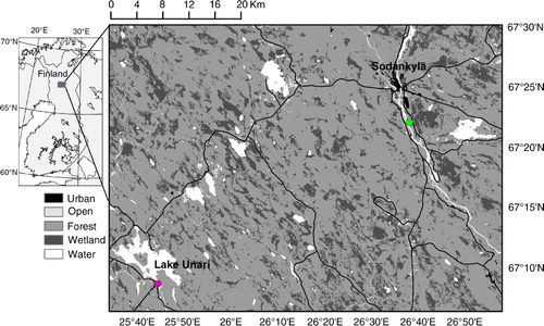
Fig. 1 The study region in northern Finland. The green and red dots mark the Sodankylä weather station and Lake Unari observation site, respectively.

The weather station data from the beginning of 1980 to the end of 2013 are used in this study. The air temperature (T_a) and relative humidity (Rh) were measured at the height of 2 m. The wind speed (V_a) and wind direction measurements were taken at the height of 22 m, which was 10 m above the forest canopy top. The measurements of V_a, T_a and Rh were made every 3 h before 2008, and since 2008 every 10 min. The total precipitation (PrecT), total cloud fraction (Cn) and snow depth on land (H_SL) were measured manually until 4 February 2008; since then the station has been equipped with automatic instrumentation. Precipitation intensity (mm/h) has been measured by FD12P weather station (Vaisala) and precipitation amount (mm) by Pluvio2 weighting gauge. For model forcing, all the weather parameters used in this study were linearly interpolated to 1-h intervals.

The long-term in situ freezing and break-up dates as well as snow and ice thickness were observed at Lake Unari 46 km southwest of the FMI Sodankylä weather station (Fig. 1). Unfortunately no regular meteorological measurements were taken near Lake Unari, and we therefore applied Sodankylä weather observations. In individual days, the weather between the two sites may naturally differ but, as the surroundings are similar (flat landscape with forest), we do not expect major differences in monthly and seasonal means, which are important for the seasonal evolution of the lake ice and the snow pack on top of it. This assumption is supported by a comparison of air temperatures at Sodankylä and two nearest weather stations: Kittilä 78 km northwest of Sodankylä and Pelkosenniemi 52 km southeast of Sodankylä. The monthly mean 2-m air temperatures during the ice season differed by less than 0.5° C between these three sites.

The Finnish Environmental Institute (SYKE) has conducted routine lake observations in Lake Unari since winter 1960/1961. The area of Lake Unari is 29 km² with an average depth of about 5 m. The snow and ice measurement site was located in the southern part of the lake. For safety reasons, the bi-weekly lake snow and ice measurements were carried out when ice was thick enough. To obtain data on a full seasonal variation of snow and ice thickness, the zero ice thicknesses were identified by the observed initial ice freeze-up and final break-up date and a linear interpolation was applied to generate time series of daily ice thickness. The observed snow thicknesses in early ice season and after the onset of snow melt were linearly extrapolated to generate full seasonal time series of daily snow thickness.

2.2. Thermodynamic snow and ice model

A high-resolution thermodynamic snow and ice model (HIGHTSI) was used to simulate snow and ice thicknesses. The HIGHTSI model was initially developed for sea ice thermodynamic modelling (Launiainen and Cheng, 1998), surface heat budget investigations (Vihma et al., 2002) and process studies on sea ice optical and thermal properties, as well as on snow and ice thermal coupling (Cheng et al., 2003, 2006, 2008). The model has been further developed and adapted to investigate lake snow and ice (Yang et al., 2012, 2013; Semmler et al., 2012; Cheng et al., 2014). The details of model physics for lake ice are summarised in Yang et al. (2012) and Cheng et al. (2014). The essential weather forcing factors for the model are T _a, V _a, Rh, Cn and PrecT.

The HIGHTSI model runs were carried out from 1 July to 30 June each winter during 1980/81–2012/13. The initial snow and ice thicknesses were set or restored to be 0.01 and 0.02 m, respectively. The initial freeze-up date was defined as the day when lake ice started to grow under continuous sub-freezing conditions. This is a simple approximation (Yang et al., 2012). There are, however, three different definitions for the date of freeze-up, referring to different stages of lake freezing (Palecki and Barry, 1986). The period covering these stages varies from days up to weeks depending on the lake phenomenology, such as location, size and depth. In our study, we define the freeze-up as the date when the modelled ice thickness reaches 0.05 m. We argue that such a freeze-up date refers to the earliest possible date of ice formation near the lake shore. The date when the calculated ice thickness becomes zero was the simulated break-up date.

2.3. Statistical methods

The climatological trends of observed weather variables and observed and modelled snow and ice variables were investigated using the Theil-Sen's slope estimator (e.g. Wilcox, 2001). The calculated trends were evaluated based on the non-parametric Mann-Kendall (MK) test (Mann, 1945; Kendall, 1948). The significance level of correlations was evaluated using the two-tailed t-test. With a 33-yr dataset, the threshold of correlation coefficients at 95 and 99 % confidence levels are 0.33 and 0.43, respectively. The correlation and regression between the meteorological factors and the modelled snow and ice parameters were calculated using the stepwise multilinear regression analysis.

The relationships between the average and maximum thickness of ice and snow and several large-scale atmospheric circulation indices (www.esrl.noaa.gov/psd/data/climateindices) were also investigated. The winter indices were constructed by averaging the monthly means of December, January and February (DJF) from 1980 to 2013. The composite differences of atmospheric variable fields (see below) within the region of 60° W–60° E and 50–80° N during the years of thin and thick lake ice are conducted. The seasons of thin and thick ice are defined by 1.0 standard deviation from normalised observed mean ice thickness of each winter. The atmospheric fields are 500 hPa geopotential height, 700 hPa zonal wind and 850 hPa and 2-m air temperatures. All these parameters were extracted from the ERA-Interim reanalysis (Dee et al., 2011).

3. Results

The monthly average values were calculated using hourly interpolated observations of weather variables and daily interpolated values of snow and ice thickness. The observed maximum snow and ice thicknesses were picked from the seasonal time series, while the modelled maximum snow and ice thicknesses were selected from the hourly time series. The annual means (AM) were calculated for the period from 1 July to 30 June. The ice freezing season (FS) was defined as 1 November to 30 April, and the rest of the year (1 May–31 October) refers to the warm season (WS). The count of Julian day continues between two successive years, for example, 1 January=day 366. The total precipitation (PrecT) consists of solid (snow, PrecS) and liquid (rain/sleet, PrecL) parts. During FS, the liquid precipitation largely depends on the air temperature (Auer, 1974). In northern Eurasia, the upper limit of air temperature under which snowfall may occur ranges from −1.0 to 2.5° C, depending on geographical conditions (Ye et al., 2013). For boreal lake, Yang et al. (2012) used a threshold of 0.5° C to extract PrecL from PrecT.

3.1. Long-term trends of weather, snow and ice

During FS, the inter-annual variation of weather in Sodankylä was large (Fig. 2). The statistical analysis of trends is summarised in Table 1. T _a , and Rh reveal increasing trends (statistical significance, p<0.05), whereas V _a on top of canopy shows a decreasing trend (p<0.05), and Cn has an insignificant decreasing trend. The PrecT has an insignificant increasing trend versus an insignificant decreasing trend of H_SL. The PrecL has an increasing trend (p=0.05) versus an insignificant decreasing trend of PrecS.

Fig. 2 The inter-annual variations of freezing season mean (blue dots) weather forcing factors of (a) wind speed, (b) air temperature, (c) relative humidity, and (d) liquid precipitation. The linear trends reach a statistical significance (p<0.05).

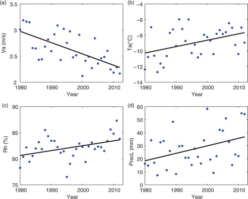
Table 1. Significance of trends (Mann-Kendall test) of meteorological parameters during the freezing season

Variable	Theil-Sen's slope (10 yr)^−1	p
T a (°C)	1.03	0.02
Rh (%)	0.83	0.01
V a (m/s)	−0.21	0.00
Cn (%)	−0.01	0.53
PrecT (mm)	7.30	0.46
PrecL (mm)	4.73	0.05
PrecS (mm)	−0.05	0.99
HSL (mm)	−7.01	0.70

p: significant probability. A positive slope indicates an increasing trend. Bold numbers: trends reach significance level (p<0.05). Cn: total cloud fraction; H_SL: snow depth on land; PrecL: precipitation liquid; PrecS: precipitation solid; PrecT: total precipitation; Rh: relative humidity; T _a : air temperatures; V _a : wind speed.

The increasing trends of air temperature were larger in early winter months than in spring. The T _a trends of 1.00, 0.79 and 0.49° C per decade were calculated for FS, AM and WS, respectively, and Rh has increased (p<0.05) in early winter months (November–January). The V _a has an overall decreasing trend during FS; the decreasing trends in November, February, March and April reached statistical significance. The decreasing of wind speed weakens the surface sensible heat flux. The monthly Cn shows no significant change, except a decreasing trend (p<0.05) in March. An increasing PrecT trend appears for all FS months but without reaching a statistical significance. In November, December and April, T_a strongly affects PrecL, but only weakly PrecS. In January and February, both PrecT and PrecS have slightly increased.

The average freeze-up day (the entire lake is frozen) observed by SYKE was 305 (1 November)±11 (mean±standard deviation), and the earliest and latest freeze-up days were 283 (10 October) and 326 (21 November), respectively. The average break-up date was 507 (22 May)±8, and the earliest and latest break-up date were 495 (10 May) and 525 (9 June), respectively. The average length of the ice season was 203±10 d. The maximum and average snow and ice thicknesses are given in Fig. 3. The decreasing trends of maximum and average ice thickness are 5 cm/decade and 3 cm/decade, respectively, both reaching statistical significance (Table 2).

Fig. 3 Observed maximum and average ice (red) and snow (blue) thicknesses in Lake Unari for winter seasons from 1980/1981 to 2012/2013. The black lines are linear trends (solid line: p<0.05; broken line: p>0.05).

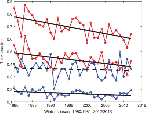
Table 2. Significance of trends (Mann-Kendall test) and Theil-Sen's slope calculation for observed and HIGHTSI modelled average and maximum seasonal snow and ice thicknesses

	Theil-Sen's slope (decade)		p
Parameters	Observed	Calculated	Observed	Calculated
H imax (cm)	−5.87	−5.17	0.00	0.01
H iave (cm)	−3.21	−3.17	0.00	0.00
H smax (cm)	−1.06	−0.92	0.43	0.23
H save (cm)	−0.98	−0.52	0.08	0.21

H _iave: seasonal average ice thickness; H _imax: seasonal maximum ice thickness; H _save: seasonal average snow thickness; H _smax: seasonal maximum snow thickness.

The observed average ice thickness is negatively correlated with FS air temperature (r=−0.50) and relative humidity (r=−0.62), and positively correlated with FS wind speed (r=0.50). All of the correlations reach 99 % significance level.

3.2. Long-term variation of modelled snow and ice parameters

The modelled snow and ice thicknesses for the 33 ice seasons are given in Fig. 4a. The modelled initial freeze-up occurred on day 300 (27 October)±12 (mean±standard deviation); the onset of snow melt occurred on day 460 (5 April)±10; the ice became snow-free on day 483 (28 April)±7, and the final break-up took place on day 518 (3 June)±8. Meanwhile, the maximum ice thickness occurred on day 461 (6 April)±19 (mean±standard deviation), and the average ice thicknesses prior to that date was 0.42 m, and 0.44 m after it. The modelled average freeze-up date was 5 d earlier than the observed one, while the modelled break-up date was 10 d later than the observed one. The modelled early freeze-up most likely results from the simple ice initialisation procedure (Yang et al., 2012), and the late break-up is probably due to the fact that winds and currents can enhance the ice floe break-up, but these dynamical processes were not considered in our model. The modelled average ice season length of 218±10 d matched the observed value within 15±10 d.

Fig. 4 (a) Time series of modelled snow and ice thickness (black dotted lines) for 33 ice seasons (1980/1981–2012/2013). The red lines are average thicknesses of snow (upper) and ice. (b) Time series of modelled maximum and average ice (red) and snow (blue) thicknesses. The black lines are linear trends (solid line: p<0.05; dashed line: p>0.05).

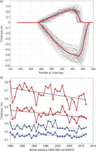
The inter-annual variations of modelled average and maximum snow and ice thicknesses are shown in Fig. 4b. The seasonal (1 November–30 April) average snow thickness was 0.15±0.02 m. The maximum snow thickness had a large inter-annual variation ranging from 0.18 to 0.34 m with an average of 0.25 m. The MK test and Theil-Sen's slope estimation are given in Table 2. Significant trends were detected for average and maximum ice thickness, but not for snow thickness. The seasonal average ice thickness was 0.42±0.06 m. The modelled maximum ice thickness ranged from 0.46 to 0.81 m with a mean value of 0.66 m. The modelled ice thickness showed a decreasing trend, which agrees with observations. The statistical analyses between observed and simulated inter-annual variation of snow and ice thickness are summarised in Table 2. The modelled mean snow and ice thickness for 1980/1981–2012/2013 as well as the maximum ice thickness during the same period all had a small bias (Table 3). The bias of modelled maximum snow thickness was larger. This may be due to the effect of wind and drifting snow, which was not taken into account in the model simulations.

Table 3. A comparison between observed and simulated maximum and average snow and ice thicknesses for the entire period 1980/1981–2012/2013

Variables	Observed (m)	Calculated (m)	r	RMSE (m)
H imax (m)	0.69	0.66	0.51	0.09
H smax (m)	0.35	0.25	0.44	0.12
H iave (m)	0.43	0.42	0.55	0.03
H save (m)	0.17	0.15	0.48	0.06

The correlation coefficient (r) and root mean square error (RMSE) between observed and simulated inter-annual time series are also given. H _iave: seasonal average ice thickness; H _imax: seasonal maximum ice thickness; H _save: seasonal average snow thickness; H _smax: seasonal maximum snow thickness.

The correlation coefficients between meteorological parameters and modelled ice components are shown in Table 4. The modelled ice thickness was correlated mainly with air temperature, snow precipitation and wind. Low temperatures associated with mild snowfall favoured columnar ice growth, whereas strong winds associated with heavy snowfall favoured the formation of granular ice.

Table 4. The correlation coefficients between meteorological parameters and modelled columnar, granular and total ice thickness

	T a	V a	Cn	PrecT	PrecS	PrecL
Granular ice	0.11	0.40	0.19	0.70	0.80	0.01
Columnar ice	−0.50	−0.24	−0.24	−0.56	−0.58	−0.19
Total ice	−0.58	0.12	−0.13	−0.01	0.08	−0.26

The significant values (p<0.05) are marked in bold. Cn: total cloud fraction; PrecL: precipitation liquid; PrecS: precipitation solid; PrecT: total precipitation; T _a : air temperatures; V _a : wind speed.

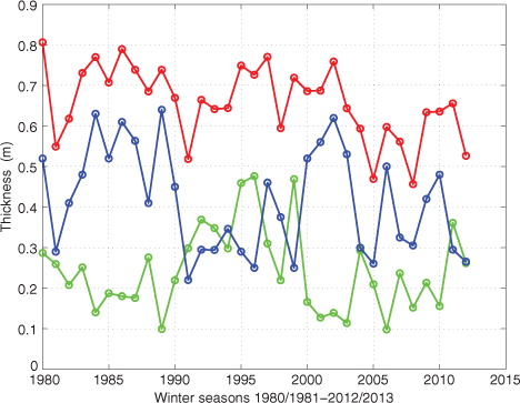
The modelled maximum ice thickness and the portions of columnar and granular ice are illustrated in Fig. 5. The portions of columnar and granular ice showed inter-annual variation. Columnar ice composed a major part of the lake ice in the 1980s. The modelled maximum ice thickness was highest in winter 1986/1987. The difference in the ratio of columnar and granular ice thickness was reduced in 1990s but increased again in 2000s. The composition of granular ice has an increasing trend since 2006.

Fig. 5 Time series of the seasonal maximum modelled total (red), columnar (blue) and granular (green) ice thickness.

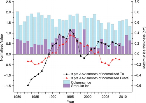
In order to see the impact of T _a and PrecS on decadal variation of lake ice compositions, a 9-yr adjacent-averaging of Ta and PrecS is calculated and compared with ice thickness products (Fig. 6). The low air temperatures associated with less precipitation yielded the columnar ice dominating in 1980s. From late-1980s to mid-1990s, the increase of granular ice was associated with more precipitation. In 2000s, the combined effect of less precipitation and higher temperatures enlarged the ratio of modelled columnar and granular ice components, and their inter-annual variations increased.

Fig. 6 The normalised 9-yr Adjacent Average (AAv) smooth values of air temperature and snow precipitation for the freezing season, and seasonal maximum ice thickness and its components (columnar and granular ice).

Synoptic weather analyses suggested that in our research domain a weak easterly wind was often accompanied with a cold high-pressure centre in western Siberia, whereas strong southerly and northerly winds were often associated with cyclone activities. This resulted in a positive correlation between the air temperature and wind speed as well as between the air temperature and cloudiness during most part of FS. A combined effect of cyclones, strong winds, warm air, more clouds and more precipitation resulted in a formation of granular lake ice, and eventually contributed positively to the total ice thickness.

Unfortunately, SYKE has no observations of the onset of snow melt on the lake. The observed snow accumulation (Hs>0.02 m) on land started on day 301 (28 October)±13, and the onset day of land-snow melt was 460±11. The observed first day with snow-free land was 499 (14 May)±8. The correlation coefficient between the onset day of land-snow accumulation and modelled lake freeze-up date was 0.81. The correlation coefficient between the first snow-free day on land and the corresponding modelled value on lake ice was 0.75. The observed onset of snow melt on land and the modelled melt onset on lake ice occurred in the same day, on average, and the correlation coefficient was as high as 0.89. This suggests that atmospheric and solar forcing, which are practically the same over the lake ice and surrounding land, dominate the timing of snow melt onset.

3.3. Regression between weather forcing factors and modelled snow and ice properties

The maximum and average values of snow and ice thickness, the granular and columnar ice thickness as well as the dates of onset of snow melt, snow-free and final ice break-up are key parameters on a seasonal scale. The variations of these parameters are closely linked with meteorological conditions. The regression equations found are presented in Table 5, and interpreted below. The seasonal maximum snow thickness (H _smax) is largely tied with the precipitation history. The total precipitation during the FS is the most important factor, followed by the air temperature. A low average FS air temperature gives a positive impact to H _smax. A low seasonal temperature may enhance ice formation and consequently retain snowfall to be accumulated on top of ice rather than turn into slush to form snow-ice. More liquid precipitation in March results in a smaller H _smax, partly because more rain in March causes densification of snow. In addition, rain in March is associated with anomalously high air temperatures, favouring snowmelt, further enhanced by the reduction of snow albedo due to rain. As expected, the seasonal maximum ice thickness (H _imax) is negatively correlated with the average air temperature in the FS. The total precipitation in February and snow precipitation in January also affect H _imax. More precipitation in these months favours snow-to-ice transformation and eventually gives a positive impact to the seasonal maximum ice thickness.

Table 5. Linear regression equations between weather forcing factors and snow and ice physical parameters

Snow and ice parameters	Regression equation	r ^2
H smax (m)	H smax=0.001·PrecT(FS)−0.01·T a(ave_FS)−0.003·PrecL(Mar.)+0.03	0.77
H imax (m)	H imax=−0.034·T a(ave_FS)+0.002·PrecT(Feb.)+0.002·PrecS(Jan.)+0.23	0.58
H save (m)	H smax=3.5e^−4·PrecT(FS)−0.003·Ta(ave_Nov.)+0.001·PrecS(Dec.)−0.001·T a(ave_Dec.)+0.04	0.86
H iave (m)	H iave=−0.03·T a(ave_FS)−0.002·PrecS(Nov.)+0.001· PrecT(Feb.)+0.04·V a(ave_Jan.)+0.14	0.73
H gi (m)	H gi=0.002·PrecT(FS)−0.12	0.63
H ci (m)	H ci=−0.005·PrecS(Nov.)−0.004·PrecS(Dec.)−0.03·T a(ave_FS)+0.50	0.72

In the equations, the forcing variables are presented in an order based on their standardised regression coefficients (the strongest factors first). See the text for definitions of the symbols. ave: average value; FS: freezing season. For precipitation, the value refers to monthly accumulation; H _iave: seasonal average ice thickness; H _imax: seasonal maximum ice thickness; H _save: seasonal average snow thickness; H _smax: seasonal maximum snow thickness; H _gi: modelled granular ice; H _ci: modelled columnar ice.

The FS air temperature has a stronger effect on the seasonal average ice thickness (H _iave) than on the seasonal maximum ice thickness (H _imax). H _iave is negatively correlated with snow precipitation in November. Heavy snowfall in early winter introduces a strong insulating effect, reducing the ice growth from the bottom. In February, the increase of total precipitation contributes to the formation of snow-ice and superimposed ice, which leads to a larger seasonal average ice thickness. The positive contributions of strong winds in January and high air temperatures in February are probably due to the fact that such conditions are typically related cyclone activity favouring formation of granular ice.

The seasonal average snow thickness (H _save) reaches its highest values in cold winters with a lot of total precipitation and snow fall. The FS average total precipitation is the most important factor, but in December, when rain is still common in some years, it is important that the precipitation falls as snow. The role of low air temperature is particularly important in November and December, so that a thick ice cover will form early enough, supporting the snow pack and reducing snow-to-ice transformation.

The modelled granular ice is largely controlled by the total precipitation in the winter season. The modelled columnar ice (H _ci) is, however, reduced by snowfall during the early winter season. More snowfall in early winter first reduces the columnar ice formation due to insulating effect of snow, and then favours granular snow-ice formation due to the heavy snow load on top of ice.

The observed snow and ice thicknesses in winter seasons after 2012/2013 were used to validate selected regression equations (Table 6). The relative errors of seasonal prognostic mean snow and ice thickness were between 9 and 12 % for 2013/2014 and 2014/2015 seasons. The relative errors for maximum snow and ice thickness were small (1–2 %) for 2014/2015 but larger for other seasons.

Table 6. The observed and prognostic snow and ice thicknesses for winter seasons after 2012/2013

	Snow thickness (cm)						Ice thickness (cm)
	H smax			H save			H imax			H iave
	Ob	Progn	Re. err. (%)	Ob	Progn	Re. err. (%)	Ob	Progn	Re. err. (%)	Ob	Progn	Re. err. (%)
2013/2014	29	29	0	17	18	12	55	54	2	39	35	10
2014/2015	46	30	34	18	20	12	60	54	10	44	40	9
2015/2016	34	37	9	14	18	28	71	60	16	54	38	29

Ob: observed value; Progn: prognostic values by regression equation; Re. err: relative error; H _iave: seasonal average ice thickness; H _imax: seasonal maximum ice thickness; H _save: seasonal average snow thickness; H _smax: seasonal maximum snow thickness.

3.4. Large-scale atmospheric circulation and lake ice phenology

The correlations between winter large-scale indices and observed meteorological and snow/ice variables for November–April in 1980/1981–2012/2013 were examined (Table 7). The role of Arctic Oscillation (AO) and NAO on the ice climate in Northern Europe has already been investigated in several studies [see Vihma and Haapala (2009) for a review]. In this study, we found that AO, NAO and the Pacific Decadal Oscillation (PDO) were correlated with a few meteorological parameters, whereas the Pacific/North American (PNA) pattern and El Niño/Southern Oscillation (ENSO) had no statistically significant correlations with weather conditions. Although correlated with meteorological variables, the NAO, among others, was not correlated with snow and ice thickness in Lake Unari. A similar result has been obtained for Lake Kilpisjärvi in the north-western part of Finland, close to the Norwegian Sea (Lei et al., 2012). Only PDO was statistically correlated with the average ice thickness in Lake Unari (Table 6). The PDO represents the leading principal component of the North Pacific (north of 20° N) monthly sea surface temperature variability. In general, when PDO is positive, the wintertime Aleutian Low is getting deeper and shifted southwards. The strong correlations between PDO and meteorological parameters as well as snow and ice variables in the Bay of Bothnia in the Northern Baltic Sea have been first discovered by Vihma et al. (2014). The physical mechanism for the linkage may be related to a planetary wave train from the Pacific across the central Arctic to Europe (Trenberth and Fasullo, 2013) or to a zonal, eastward propagating wave train (Zhao et al., 2004). These wave trains originate from the thermal forcing from the North Pacific sea surface temperature anomalies to the atmosphere.

Table 7. The correlation coefficients between large-scale circulation indices and meteorological parameters, snow and ice thickness

	V a	T a	Rh	Cn	PrecT	PrecS	PrecL	H iave	H imax	H save	H smax
AO	0.45	0.50	0.07	0.16	0.28	0.33	−0.03	0.05	0.13	−0.07	−0.14
PNA	−0.16	−0.10	−0.09	0.32	0.04	0.05	−0.00	−0.05	−0.12	0.10	0.36
NAO	0.43	0.44	0.00	0.39	0.35	0.42	−0.06	0.08	0.05	0.08	0.00
PDO	0.06	−0.51	−0.36	0.15	−0.23	−0.24	−0.04	0.41	0.29	0.15	0.03

Significant values (p<0.05) are marked as bold. AO: Arctic oscillation; Cn: total cloud fraction; H _iave: seasonal average ice thickness; H _imax: seasonal maximum ice thickness; H _save: seasonal average snow thickness; H _smax: seasonal maximum snow thickness; NAO: North Atlantic Oscillation; PDO: Pacific Decadal Oscillation; PNA: Pacific/North American pattern; PrecL: precipitation liquid; PrecS: precipitation solid; PrecT: total precipitation; Rh: relative humidity; T _a : air temperatures; V _a : wind speed.

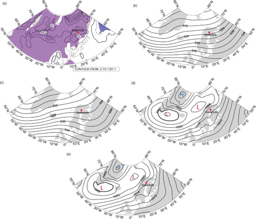
Compared with winters with thick ice, winters with thin ice in Lake Unari were associated with higher 2-m air temperatures over a broad region covering most of the sea areas north of 50° N from the coast of North America to Novaya Zemlya, as well as land areas of Greenland and northern Fenno-Scandia (Fig. 7a). Such a pattern suggests that the local temperatures over Lake Unari were strongly controlled large-scale atmospheric circulation. Comparing 500 hPa geopotential heights averaged over winters of thick (Fig. 7b) and thin lake ice (Fig. 7c), we see, however, that the geopotential height gradient over Sodankylä was, surprisingly, weaker in years of thin ice, indicating weaker mid-tropospheric zonal winds. The mean-sea-level pressure (MSLP) was, also surprisingly, slightly (1.5 hPa) higher in winters with thin lake ice (compare Fig. 7d and e). The MSLP gradient over Sodankylä was, however, stronger in winters with thin ice, indicating stronger south-westerly geostrophic winds, advecting warm air masses to Sodankylä, which seems to be the aspect of the large-scale forcing that explains the differences in the 2-m air temperature and lake ice thickness.

Fig. 7 The composite difference (value of thin ice season subtract value of thick ice season) of winter means (DJF) values of 2-m air temperature (a); the large-scale atmospheric circulation pattern of 500 hPa geopotential height averaged over years of thick (b) and thin (c) ice seasons; the mean-sea-level pressure averaged over years of thick (d) and thin (e) ice season. The shaded areas in (a) indicate 95 % confidence level. The violet and blue colours represent positive and negative composite differences, respectively. The seasons of thick lake ice are 1980/1981, 1983/1984, 1984/1985, 1985/1986, 1992/1993, 1997/1998, and those of thin lake ice are 1991/1992, 2000/2001, 2005/2006, 2010/2011, 2011/2012.

4. Conclusions

Meteorological conditions and their effects on snow and ice thickness in Lake Unari were investigated for winters 1980/1981–2012/2013. The air temperature during FS had an increasing trend over the study period, in particular in November and December. The wind speed had a decreasing trend during FS. The air relative and specific humidity had increased in November, December and January, but cloudiness had decreased in March, increasing the downward solar radiation. The air temperature, wind speed, cloudiness and total precipitation were correlated with NAO. The decrease of wind speed was connected to a decrease in the NAO index, which may be partly related to the Arctic sea ice decline (Vihma, 2014).

We discovered that among large-scale climate indices, PDO was the only one that correlated with inter-annual variations in the seasonal average ice thickness in Lake Unari. This relationship may be generated by planetary wave trains exited by sea surface temperature anomalies in the North Pacific. The NAO index was not correlated with snow and ice thickness in Lake Unari.

The HIGHTSI modelled snow and ice thickness were comparable with the observations, in particular the inter-annual variations of maximum and average ice thickness correlated with the observed values. HIGHTSI was able to calculate seasonal ice thickness compositions. Inter-annual variations in the portions of columnar and granular ice were be mostly explained by variations of air temperature and the amount and phase of precipitation. Granular (columnar) ice thickness was positively (negatively) correlated with precipitation.

The HIGHTSI modelled average seasonal freeze-up date was close to the observed value. The result from simple calculation procedure of initial freeze-up of Yang et al. (2012) can be regarded as the earliest possible date of ice freezing in a shallow lake. Neglecting of lake hydrological processes, such as mixing, could naturally lead to too early freeze-up. The delay of modelled average ice break-up date was probably caused by the missing of dynamic break-up mechanism in the model. In reality, the final phase of ice break-up is strongly affected by winds and currents (Lei et al., 2010).

The modelled average snow and ice thicknesses as well as maximum ice thickness agreed well with the observed values. The model results were better for ice than snow and more accurate for seasonal means than maxima. The modelled maximum snow thickness was far from the observed one. This is partly due to the uncertainty of precipitation and coarse temporal resolution of observations. The model, however, performed well in simulating the spring onset of snow melt.

The seasonal mean and maximum lake ice and snow thicknesses were controlled by precipitation and temperature history, with 58–86 % of the inter-annual variance explained. Ice break-up in spring was delayed by low temperatures and thick snow pack on top of ice. The multilinear regression analyses provided some insights on the relationships between seasonal weather variables and lake snow and ice phenology. Although possibilities for seasonal weather forecasts in high latitudes are very limited, the heat capacity of the lake water in autumn generates some potential for seasonal prediction of freeze-up, and the heat capacity and latent heat of melting of lake ice and snow generate some potential for seasonal prediction of ice and snow thickness as well as the snow melt and ice break-up. Using the regression equations derived from data from 1980 to 2013, we made a first trial to forecast snow and ice thickness for the following winter seasons. The forecasts included errors of 9–12 % in snow and ice thickness for winters 2013/2014 and 2014/2015. The errors for maximum snow and ice thickness were small (1 to 2 %) for winter 2014/2015. In order to improve regression equations for seasonal forecasting of snow and ice thickness, the time series of data sets (1980/1981–2012/2013) need to be extended.

More effort is needed to better characterise the physical relationships between weather variables, and snow and ice thermodynamics in Arctic lakes. Such an effort may have potential applications, for example, to improve the accuracy of representation of lake snow and ice in NWP and climate models.

5. Acknowledgements

This study was financially supported by the Natural Science Foundation of China under the contracts 41428603 and 41206186, the Academy of Finland (contract 283101) and ‘Nordic Snow Radar Experiment’ project funded by ESA. SYKE is acknowledged for providing snow and ice measurements for Lake Unari. Comments from two anonymous reviewers were very helpful and led to significant improvements of the manuscript.

References

- Auer A. H . The rain versus snow threshold temperatures. Weatherwise. 1974; 27: 67.
- Bring A., Fedorova I., Dibike Y., Hinzman L., Mård J., co-authors. Arctic terrestrial hydrology: a synthesis of processes, regional effects, and research challenges. J. Geophys. Res. Biogeosci. 2016; 121: 621–649. DOI: http://dx.doi.org/10.1002/2015JG003131.
- Cheng B. , Vihma T. , Launiainen J . Modelling of the superimposed ice formation and sub-surface melting in the Baltic Sea. Geophysica. 2003; 39: 31–50.
- Cheng B. , Vihma T. , Pirazzini R. , Granskog M . Modeling of superimposed ice formation during spring snowmelt period in the Baltic Sea. Ann. Glaciol. 2006; 44: 139–146.
- Cheng B., Zhang Z., Vihma T., Johansson M., Bian L., co-authors. Model experiments on snow and ice thermodynamics in the Arctic Ocean with CHINAREN 2003 data. Geophys. Res. 2008; 113 C09020. DOI: http://dx.doi.org/10.1029/2007JC004654.
- Cheng B., Vihma T., Rontu L., Kontu A., Kheyrollah P. H., co-authors. Evolution of snow and ice temperature, thickness and energy balance 1 in Lake Orajärvi, northern Finland. Tellus A. 2014; 66 21564. DOI: http://dx.doi.org/10.3402/tellusa.v66.21564.
- Dee D. P., Uppala S. M., Simmons A. J., Berrisford P., Poli P., co-authors. The ERA-Interim reanalysis: configuration and performance of the data assimilation system. Q. J. Roy. Meteorol. Soc. 2011; 137: 553–597. DOI: http://dx.doi.org/10.1002/qj.828.
- Efremova T., Palshin N., Zdorovennov R. Long-term characteristics of ice phenology in Karelian lakes. Estonian. J. Earth Sci. 2013; 62: 33–41. DOI: http://dx.doi.org/10.3176/earth.2013.04.
- George D. G. , Järvinen M. , Arvola L . The influence of the North Atlantic Oscillation on the winter characteristic of Windermere (UK) and Pääjärvi (Finland). Boreal. Env. Res. 2004; 9: 389–399.
- Heino R. , Tuomenvirta H. , Vuglinsky V. S. , Gustafsson B. G. , Alexandersson H. , co-authors . Past and current climate change. Assessment of Climate Change for the Baltic Sea Basin. 2008; 35–131. Springer Verlag, Berlin ed. BACC Author Team.
- Jensen O. P. , Benson B. J. , Magnuson J. J. , Virginia M. C. , Martyn N. F. , co-authors . Spatial analysis of ice phenology trends across the Laurentian Great Lakes region during a recent warming period. Limnol. Oceanogr. 2007; 52(5): 2013–2026.
- Johannessen O. M., Kuzmina S. I., Bobylev L. P., Miles M. M. Surface air temperature variability and trends in the Arctic: new amplification assessment and regionalization. Tellus A. 2016; 68 28234. DOI: http://dx.doi.org/10.3402/tellusa.v68.28234.
- Kangas M., Rontu L., Fortelius C., Aurela M., Poikonen A. Weather model verification using Sodankylä mast measurements. Geosci. Instrum. Method. Data. Syst. 2016; 5: 75–84. DOI: http://dx.doi.org/10.5194/gi-5-75-2016.
- Kendall M. G . Rank Correlation Methods. 1948; London: Griffin.
- Kuusisto E. , Elo A. R . Lake and river ice variables as climate indicators in Northern Europe. Verh. Internat. Verein. Limnol. 2000; 27(5): 2761–2764.
- Launiainen J. , Cheng B . Modelling of ice thermodynamics in natural water bodies. Cold Reg. Sci. Technol. 1998; 27(3): 153–178.
- Lei R., Li Z., Cheng B., Zhang Z., Heil P. Annual cycle of landfast sea ice in Prydz Bay, east Antarctica. J. Geophys. Res. 2010; 115 C02006. DOI: http://dx.doi.org/10.1029/2008JC005223.
- Lei R., Leppäranta M., Cheng B., Heil P., Li Z. Changes in ice-season characteristics of a European Arctic lake from 1964 to 2008. Clim. Change. 2012; 115 725. DOI: http://dx.doi.org/10.1007/s10584-012-0489-2.
- Mann H. B . Nonparametric tests against trend. Econometrica. 1945; 13(3): 245–259.
- Palecki M. A. , Barry R. G . Freeze-up and break-up of lakes as an index of temperature changes during the transition seasons: a case study for Finland. J. Appl. Meteorol. Climatol. 1986; 25: 893902.
- Prowse T., Alfredsen K., Beltaos S., Bonsal B., Duguay C., co-authors. Past and future changes in Arctic lake and river ice. Ambio. 2011; 40: 53–62. DOI: http://dx.doi.org/10.1007/s13280-011-0216-7.
- Prowse T. D. , Brown K . Hydro-ecological effects of changing Arctic river and lake ice covers: a review. Hydrol. Res. 2010; 41: 454–461.
- Saloranta T . Modelling the evolution of snow, snow ice and ice in the Baltic Sea. Tellus A. 2000; 52: 93–108.
- Semmler T., Cheng B., Yang Y., Rontu L. Snow and ice on Bear Lake (Alaska) – sensitivity experiments with two lake ice models. Tellus A. 2012; 64 17339. DOI: http://dx.doi.org/10.3402/tellusa.v64i0.17339.
- Surdu C. M., Duguay C. R., Brown L. C., Fernandez Prieto D. Response of ice cover on shallow lakes of the North Slope of Alaska to contemporary climate conditions (1950–2011): radar remote-sensing and numerical modelling data analysis. Cryosphere. 2014; 8 167180. DOI: http://dx.doi.org/10.5194/tc-8-167-2014.
- Tietäväinen H., Tuomenvirta H., Venäläinen A. Annual and seasonal mean temperatures in Finland during the last 160 years based on gridded temperature data. Int. J. Climatol. 2010; 30: 2247–2256. DOI: http://dx.doi.org/10.1002/joc.2046.
- Tikkanen M . Seppälä M . Climate. The Physical Geography of Fennoscandia. 2005; Oxford: Oxford University Press. 96–112.
- Trenberth K. E., Fasullo J. T. An apparent hiatus in global warming?. Earth's. Future. 2013; 1: 19–32. DOI: http://dx.doi.org/10.1002/2013EF000165.
- Tuomenvirta H. , Alexandersson H. , Drebs A. , Frich P. , Nordli P. O . Trends in Nordic and Arctic temperature extremes and ranges. J. Clim. 2000; 13: 977–990.
- Vihma T. Effects of Arctic sea ice decline on weather and climate: a review. Surv. Geophys. 2014; 35: 1175. DOI: http://dx.doi.org/10.1007/s10712-014-9284-0.
- Vihma T., Cheng B., Uotila P., Wei L., Qin T. Linkages between Arctic sea ice cover, large-scale atmospheric circulation, and weather and ice conditions in the Gulf of Bothnia, Baltic Sea. Adv. Polar. Sci. 2014; 25: 289–299. DOI: http://dx.doi.org/10.13679/j.advps.2014.4.00289.
- Vihma T., Haapala J. Geophysics of sea ice in the Baltic Sea – a review. Progr. Oceanogr. 2009; 80: 129–148. DOI: http://dx.doi.org/10.1016/j.pocean.2009.02.002.
- Vihma T., Screen J., Tjernström M., Newton B., Zhang X., co-authors. The atmospheric role in the Arctic water cycle: a review on processes, past and future changes, and their impacts. J. Geophys. Res. Biogeosci. 2016; 121: 586–620. DOI: http://dx.doi.org/10.1002/2015JG003132.
- Vihma T., Uotila J., Cheng B., Launiainen J. Surface heat budget over the Weddell Sea: Buoy results and model comparisons. J. Geophys. Res. 2002; 107(C2): 3013. DOI: http://dx.doi.org/10.1029/2000JC000372.
- Wilcox R. R . Fundamentals of Modern Statistical Methods: Substantially Improving Power and Accuracy. 2001; Los Angeles, CA: Springer-Verlag.
- Yang Y. , Cheng B. , Kourzeneva E. , Semmler T. , Rontu L. , co-authors . Modelling experiments on air–snow–ice interactions over Kilpisjärvi, a lake in northern Finland. Boreal. Env. Res. 2013; 18: 341–358.
- Yang Y., Leppäranta M., Cheng B., Li Z. Numerical modelling of snow and ice thickness in Lake Vanajavesi, Finland. Tellus A. 2012; 64 17202. DOI: http://dx.doi.org/10.3402/tellusa.v64i0.17202.
- Ye H. , Cohen J. , Rawlines M . Discrimination of solid from liquid precipitation over Northern Eurasia using surface atmospheric condition. J. Hydrometeorol. 2013; 14: 1345–1355.
- Zhao P. , Zhang X. , Zhou X. , Ikeda M. , Yin Y . The sea ice extent anomaly in the North Pacific and its impact on the East Asian summer monsoon rainfall. J. Clim. 2004; 17: 3434–3447.