Flow-dependent assimilation of sea surface temperature in isopycnal coordinates with the Norwegian Climate Prediction Model

Abstract

We document a pilot stochastic re-analysis computed by assimilating sea surface temperature (SST) anomalies into the ocean component of the coupled Norwegian Climate Prediction Model (NorCPM) for the period 1950–2010 (doi: 10.11582/2016.00002). NorCPM is based on the Norwegian Earth System Model and uses the ensemble Kalman filter for data assimilation (DA). Here, we assimilate SST from the stochastic HadISST2 historical reconstruction. The accuracy, reliability and drift are investigated using both assimilated and independent observations. NorCPM is slightly overdispersive against assimilated observations but shows stable performance through the analysis period. It demonstrates skills against independent measurements: sea surface height, heat and salt content, in particular in the Equatorial and North Pacific, the North Atlantic Subpolar Gyre (SPG) region and the Nordic Seas. Furthermore, NorCPM provides a reliable monitoring of the SPG index and represents the vertical temperature variability there, in good agreement with observations. The monitoring of the Atlantic meridional overturning circulation is also encouraging. The benefit of using a flow-dependent assimilation method and constructing the covariance in isopycnal coordinates are investigated in the SPG region. Isopycnal coordinates discretisation is found to better capture the vertical structure than standard depth-coordinate discretisation, because it leads to a deeper influence of the assimilated surface observations. The vertical covariance shows a pronounced seasonal and decadal variability that highlights the benefit of flow-dependent DA method. This study demonstrates the potential of NorCPM to compute an ocean re-analysis for the 19th and 20th centuries when SST observations are available.

• Ocean re-analysis
• EnKF
• isopycnal ocean model
• SST coupled re-analysis
• weakly coupled data assimilation
• NorCPM
• Flow dependent assimilation

1. Introduction

It is of crucial societal importance to understand the sensitivity of our climate to anthropogenic forcing. As observations of our climate are sparse and are homogeneously distributed, it is often hard to disentangle anthropogenic climate change from natural climate variability. Historical reanalyses aim to provide continuous and reliable reconstructions of past climate by fusing the scarce observations into physically consistent climate systems. They can also be used as initial conditions for predictions. Thus, they are useful for understanding the mechanisms for climate change and predictability during the historical period. While such reconstructions of the atmosphere have been available for over a decade (Kalnay et al., 1996; Dee et al., 2011), the paucity of observations makes long-term oceanic reconstructions more challenging.

Generally speaking, there are three approaches to reconstruct past ocean variability. (1) Ocean global circulation models (OGCMs) forced by atmospheric re-analysis provide a first-order reconstruction of past ocean variability (Danabasoglu et al., 2014). However, oceanic variability is not fully determined by atmospheric forcing, and there are inaccuracies in ocean models and the atmospheric forcing. (2) Assimilation of ocean observations into forced OGCMs improves on this first class of reconstruction (Carton and Giese, 2008; Köhl and Stammer, 2008; Ferry et al., 2010; Sakov et al., 2012; Karspeck et al., 2013; Oke et al., 2013; Storto et al., 2015; Zuo et al., 2015). While they can reach high levels of accuracy, they do not optimally account for the coupled dynamics of the climate system affecting the realism of the variability mechanisms. (3) Assimilating observations directly into a fully coupled earth system model can better represent the interactions between climate system components (Fujii and Kamachi, 2003; Keenlyside et al., 2005; Saha et al., 2010; Zhang et al., 2010; Swingedouw et al., 2012; Brune et al., 2015; Laloyaux et al., 2015; Mochizuki et al., 2016). The Norwegian Climate Prediction Model (NorCPM) belongs to this third class.

Coupled ocean re-analysis products differ in the choice of observations assimilated and in the complexity of the data assimilation (DA) methods employed. Zhang et al. (2010) emphasised the importance of Argo floats for constraining the ocean and demonstrated that with a modern observation network, the variability in the North Atlantic can be accurately monitored. However, apart from sea surface temperature (SST) that is available to some level of accuracy from 1850, very few observations are available before the 1990s: satellite altimetry is only available from 1993 and vertical sampling of the hydrography is only sporadically observed prior to the Argo floats programme starting in the early 2000s. Several studies have thus attempted to constrain the climate system based on SST only in order to provide a long consistent reconstruction and demonstrate the skill of initialised prediction for seasonal-to-decadal time scale. Simple nudging of coupled model SST to observations was shown to have some skill in the North Atlantic and in the tropical Pacific (Keenlyside et al., 2005, 2008; Swingedouw et al., 2012; Mignot et al., 2015). Counillon et al. (2014) attempted to use advanced DA to constrain the full-water depth from SST data with NorCPM. The low-frequency variability of the ocean was successfully controlled, and skilful decadal predictions were achieved in the North Atlantic and the Nordic Seas. However, the results were carried in a twin experiment that assumes a perfect model framework. The current study aims at demonstrating the skill of NorCPM in a realistic framework and, in particular, in its capability to provide a re-analysis. The system assimilates the HadISST2 product (Kennedy et al., 2015; Rayner et al., 2015) for the period 1950–2010, a period during which many independent observations are available for validation. By mimicking the shortage of ocean observations, we assess the potential of NorCPM for providing a re-analysis for periods during the 19th and 20th centuries when ocean observations are effectively limited to SST. Although it is clear that the current re-analysis cannot match the level of accuracy of other systems that make use of all observations (Carton and Giese, 2008; Saha et al., 2010; Zhang et al., 2010; Karspeck et al., 2013; Laloyaux et al., 2015), it does have some assets. The introduction of new types of observations in the course of a re-analysis introduces discontinuities, which are limited here. Large efforts were also made in the DA method to minimise the assimilation shocks and preserve the physical consistency of the system. The system provides a stochastic reconstruction of the climate that can be used to estimate the accuracy of the system in time and space. This re-analysis will also serve as a first prototype for initialising climate prediction for the Decadal Climate Prediction Project (DCPP) of the Coupled Model Intercomparison Project (CMIP) phase 6 (Eyring et al., 2015).

NorCPM combines the Norwegian Earth System Model (NorESM) with the ensemble Kalman filter (EnKF; Evensen, 2007) DA method. NorESM (Bentsen et al., 2012) is a state-of-the-art climate model that participated in the 5th CMIP. The model is based on the Community Earth System Model (CESM) from the National Center for Atmospheric Research, but uses an isopycnal coordinates ocean model and a different atmospheric chemistry and ocean biochemistry model. The EnKF is an advanced DA method that provides flow-dependent and multivariate covariance to extrapolate the correction to unobserved variables based on an ensemble of model states. The EnKF has several advantages for climate prediction. First, it is designed for a dynamical system such as our climate system and as such provides a more reliable covariance than a static covariance matrix (Sakov and Sandery, 2015). This becomes critical when the observational network is sparse. Second, the covariance is constructed from the model itself, which ensures that the updates satisfy the model dynamics (under the linear hypotheses) and limits the assimilation shocks (Evensen, 2003). NorCPM is not the first EnKF-based system for reconstructing our climate (Zhang et al., 2007; Karspeck et al., 2013; Brune et al., 2015). However, it has several particularities. First, the EnKF is applied to an isopycnal ocean model, which can have some advantages (Gavart and De Mey, 1997; Srinivasan et al., 2011). Second, it uses a fairly large ensemble size with 30 members in a fully coupled configuration. In Counillon et al. (2014), this ensemble size was found sufficient to avoid the need for vertical localisation. Finally, it assimilates the new HadISST2 product (Kennedy et al., 2015; Rayner et al., 2015), which provides a stochastic reconstruction of SST – that is, providing a three-dimensional estimate of the measurement and its accuracy – for the period 1850–2010.

This paper is organised as follows. Section 2 presents NorCPM, which combines NorESM (Section 2.1), the EnKF (Section 2.2) and the HadISST2 observations assimilated (Section 2.3). A global validation of the system is carried out in Section 3, against the assimilated SST product (Section 3.1) and independent measurements: the steric global mean sea level (Section 3.2), variability of sea surface height (SSH, Section 3.3), and heat and salt content variability (Section 3.4). In Section 4, we evaluate NorCPM in the North Atlantic Subpolar Gyre (SPG) region and investigate the advantages of constructing flow-dependent covariance in isopycnal coordinates there. A summary and conclusions are given in Section 5.

2. The Norwegian Climate Prediction System

2.1. The Norwegian Earth System Model

NorESM (Bentsen et al., 2012) is a global fully coupled system for climate simulations. It is based on the CESM version 1.0.3 (CESM1, Vertenstein et al., 2012), a successor to the Community Climate System Model version 4 (Gent et al., 2011). As in CESM1, NorESM uses the Community Land Model version 4 (Oleson et al., 2010; Lawrence et al., 2011) and the Los Alamos sea ice model version 4 (Gent et al., 2011; Holland et al., 2012) with the version 7 coupler (Craig et al., 2011). NorESM key differences to CESM1 are the atmospheric and the ocean components. Unlike in the Community Atmosphere Model (CAM4, Neale et al., 2010), the atmospheric component (CAM4-OSLO) features advanced aerosol chemistry schemes that also account for indirect aerosol effects (Kirkevåg et al., 2013). The ocean component (Bentsen et al., 2012) is an updated version of the Miami isopycnal coordinate ocean model (MICOM, Bleck et al., 1992). With potential density as vertical coordinates, the model layer interfaces are a good approximation to neutral surfaces and allow for minimising spurious mixing compared with other choices of vertical coordinates. This allows for an excellent preservation of water mass properties. The reference potential densities are selected to best represent characteristic water masses. Potential densities are referenced here to 2000 dbar to maximise neutrality of the isopycnal surfaces (McDougall and Jackett, 2005). When the potential density of a layer falls outside the range of its reference densities in the water column, it becomes empty or massless. The model ensures the conservation of mass (non-Boussinesq) and conservation of potential vorticity/enstrophy for the momentum equation (Sadourny, 1975). The model uses the incremental remapping algorithm (Dukowicz and Baumgardner, 2000) for the advection of layer thickness and tracer (e.g. potential temperature and salinity); this is expressed in a flux form and ensures the conservation (and monotonicity) of mass and tracers. The model uses a bulk surface mixed layer that is divided into two layers with freely evolving density. The first isopycnal layer (below the mixed layer) is not required to stay close to its prescribed reference potential density. A diapycnal diffusion scheme adjusts an isopycnal layer's potential density to its reference potential density when the two differ. For further model details, see Bentsen et al. (2012).

This study uses the medium-resolution NorESM1-ME (Tjiputra et al., 2013), which has the capability to be fully emission driven and has contributed with output to CMIP5. External forcings used here comply with CMIP5's historical experiment [see Bentsen et al., 2012, for details]. The atmosphere and land model have a resolution of 1.9×2.5 (or f19 for the approximately 2° finite volume grid). The ocean and sea ice have a horizontal resolution of approximately 1°. The ocean uses 51 isopycnal layers and 2 additional layers for representing the bulk mixed layer. Note that there is no relaxation towards climatology.

2.2. The ensemble Kalman filter

Currently, only SST is assimilated in NorCPM and it is used to update the water column below. As DA is only performed in the ocean component, the system belongs to the class of weakly coupled DA (Laloyaux et al., 2015), where the adjustment between the individual compartments occurs dynamically during the integration of the system.

The EnKF is a recursive DA method that consists of a Monte Carlo integration and a Bayesian update that uses the sample covariance matrix from the ensemble of integrations. The ensemble of N model states (X) is denoted by1

where n is the size of the model state and x contains the full model state; that is, temperature, salinity, zonal and meridional velocities, and the layer thickness in isopycnal coordinates. The method is optimal when the model and the observation error are Gaussian and unbiased, in which case the ensemble mean provides the most likely estimation (i.e. it coincides with the maximum of likelihood) and the model covariance (P) provides a reliable estimate of the forecast error :2

where the superscript T denotes a matrix transpose and A the ensemble anomaly (i.e. , with ). The analysis is performed monthly and it uses the observations (d) and their associated covariance matrix (R) to estimate a new ensemble of model states X ^a. The observation error covariance matrix R is assumed diagonal for simplicity (i.e. the observation errors are assumed uncorrelated). We use the deterministic EnKF (DEnKF; Sakov and Oke, 2008). It is a square-root (deterministic) formulation of the EnKF that solves the analysis without the need for perturbation of the observations. It overestimates the analysed error covariance by adding a semi-definite positive term to the theoretical error covariance given by the Kalman filter, which reduces the amount of inflation needed. The analysis performs the update of the ensemble mean [eq. (3)] and the update of the ensemble anomaly [eq. (4)] separately, and it reconstructs the analysis ensemble by combining the two [eq. (5)]:3 4 5

The superscript ‘a’ refers to the analysis state and ‘f’ to the forecast, and H is the measurement operator relating the prognostic model state variables to the measurements. The Kalman gain (K) is computed as follows:6

Most of the settings follow the perfect model study of Counillon et al. (2014). The full water column and all variables are updated. This ensures the conservation of the linear properties and the equality between the sum of the layer thickness and the bottom pressure for each individual member. The horizontal localisation radius is limited to the grid cell dimensions, which vary from region to region (maximum radius = 1.25°). This may introduce discontinuity in the update, but the spatial smoothness is ensured by the spatial autocorrelation of the model and the observations, which are available at every grid cell (except below the sea ice). Although our system uses the DEnKF that limits the need for inflation, some inflation is still needed to counteract ensemble spread collapse caused by sampling error and unfulfilled prior assumptions. The ensemble spread is sustained by using the moderation technique and the pre-screening method (Sakov et al., 2012). The ensemble forecast, X ^f, consists of the ensemble of restart files in the middle of the month and is compared to the monthly averaged observations (d). The analysis update is only applied to the first time level (of the leap frog scheme) and copied to the second time level to control the computational inconsistencies due to DA adjustments (see Zhang et al., 2004). The initial ensemble is generated by spinning up an ensemble of states (sampled from a long preindustrial forcing run) with real historical forcing from 1850 to 1950. This ensures that the initial ensemble spans sufficient spread in the interior of the ocean and that every member has experienced identical external forcing. In order to avoid an abrupt start of the DA spin up, the observation error variance is inflated by a factor of 8 and gradually decreased over five assimilation cycles (5 months), as proposed in Sakov et al. (2012).

Here, we use a real framework, and thus the model has biases. There are two common strategies to handle bias: full-field assimilation (with subsequent post-processing) or anomaly assimilation (on a biased model climatology). Both methods have their advantages and disadvantages; see Weber et al. (2015) for further details on the two methods. Full-field assimilation is more problematic in ensemble DA (Dee, 2005). Indeed, models are attracted to their biased climatological states, and the model bias in the observed variables gets recursively transferred to the non-observed variables by the multivariate covariance matrix, which leads to a slow degradation of the system during the analysis period. As we only assimilate one variable (SST), we decided to use anomaly assimilation. The climatological monthly mean for the observations and the model are calculated for the period 1950–2009. This assumes erroneously that only the mean state of the system is biased but not its climate sensitivity and variability; a choice that may lead to a sub-optimal analysis, but avoids transferring error to non-observed regions (typically in the deep ocean).

We also employ the aggregation method (Wang et al., 2016), which is a cost-efficient modification of the linear analysis update to reduce error in DA methods for physically constrained variables. MICOM is isopycnal in its vertical coordinates and one of its state variables – the layer thickness – varies in space and time but is always positive and, thus, has a truncated Gaussian distribution. The linear analysis update of the EnKF may inevitably return unphysical (negative) values. To remedy this, we are iteratively aggregating the variables in the vertical until no unphysical solution is returned. This approach is found to reduce the drift by a factor of 10 compared with the standard post-processing approach used in Counillon et al. (2014), and it does not impair the efficiency of assimilation. Furthermore, no other affordable solution has been proposed to preserve the mass, heat and salt content for each layer.

During the course of the re-analysis, two minor bugs were found. The first one is observation anomalies below −3 °C were discarded. The second one is observations were displaced by 1° meridionally. The sensitivity of our system to these bugs was tested by carrying out a parallel analysis (with and without the bug) for the period 1980–2010. The performance of the system and the result presented in this article were barely discernible. In the following, the result concatenates the re-analysis that has the bugs during the period 1950–1980 with the bug-free version for the period 1980–2010.

2.3. SST observations

Ten realisations of the preliminary HadISST2 data set (HadISST2.1.0.0, Rayner et al., 2015) observations have been assimilated. The data set is global and provides monthly SST (Kennedy et al., 2015) and sea ice concentration (Titchner and Rayner, 2014) from 1850 to 2010 at 1° resolution. It is based on SST from ICOADS (International Comprehensive Ocean Atmosphere Data Set, http://icoads. noaa.gov/) and from the Met Office observational database; SST retrievals from AVHRR Pathfinder V5 data (1985–2007); and SST retrievals from the ATSR2 and AATSR (1995–2011) METEO products. The in-situ data are bias adjusted using an updated version of Kennedy et al. (2011). The ensemble samples the accuracy of the analysis by perturbing uncertain parameters. We use the ensemble spread to quantify the accuracy of the data set, which allows for time and space varying estimation of its accuracy. Furthermore, we assume that observation errors are decorrelated [i.e. R in eq. (6) is diagonal].

3. Global validation

Here, we assess the performance of NorCPM by comparing the monthly averaged re-analysis against the assimilated measurements (SST) and other independent measurements such as sea level, heat content (HC) and salt content (SC). NorCPM is compared to a corresponding 30-member ensemble integrated forward from the same initial conditions in 1950 and with the same external forcing as NorCPM, but without assimilation (hereafter referred as FREE). FREE would correspond to a typical climate projection exercise where the system is constrained only by the external forcing.

3.1. Assimilated SST

The performance of NorCPM in monitoring the variability of SST is assessed in terms of root mean square error (RMSE) and bias, and by comparing against FREE. NorCPM is expected to show less error than FREE, because the assessment is against the very same assimilated SST data. Nevertheless, the comparison is useful to assess the accuracy of the system over time. The statistics are computed using monthly averaged SST anomalies (w.r.t. the same 1950–2009 climatology used in the assimilation). The RMSE and the bias are calculated from the ensemble mean of NorCPM, FREE and observations. We also assess the reliability of NorCPM. The reliability is defined as the capability of the system to estimate its accuracy – the ensemble spread (the standard deviation of the ensemble) being used to quantify uncertainty.

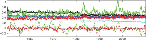
DA reduces the RMSE and the bias consistently throughout the whole study period, with no obvious degradation (Fig. 1). There are pronounced maxima of RMSE in FREE corresponding to the large El Niño events (in 1982–1983, 1986–1987 and 1997–1998) during which the amplitude of the anomaly of SST is larger. Overall, the performance of FREE is poorer after 1982, which coincides with the availability of satellite data. The inclusion of this new data type in HadISST2 leads to a reduction of the observation error (cyan line) that is associated with better synchronisation among the observation members. From that time, the observation ensemble mean shows larger amplitude and smaller scale spatial structures, and it becomes less comparable to FREE. Comparatively, NorCPM shows only a slight increase in RMSE post 1982. Actually, NorCPM shows lower RMSE than the observational data set before 1982 but is slightly poorer afterwards. In a perfect model framework, the error in an assimilation run would reduce with more accurate observations. However, the spatial scales of the features resolved in the observations post satellite era are smaller and their inherent predictability as well as the capability of our model to resolve them is reduced. Overall, the accuracy of NorCPM is stable with an accuracy of approximately 0.4 °C and no obvious bias.

Fig. 1 Monthly RMSE (unit is in °C for all variables) of NorCPM (thick red line) and FREE (thick green line) against the assimilated SST anomaly. The contribution of the bias in the RMSE is plotted with the dashed line. The HadISST2 accuracy (i.e. the SD) is plotted in cyan. The ensemble spread of NorCPM is in blue and the black line is σ _tot, as defined in eq. (7).

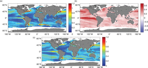
Figure 2a shows the spatial distribution of the time averaged RMSE in NorCPM. The error is low in most places (<0.4 °C) except in frontal regions where RMSE is larger than 1.2 °C with a maximum in the Gulf Stream region (1.9 °C). The reduction of error compared with FREE (RMSE_FREE - RMSE_NorCPM) is shown in Fig. 2b. NorCPM reduces error everywhere. The reduction is larger in places where the initial RMSE is large. However, the reduction is comparatively larger for the Equatorial Pacific, SPG and Kuroshio regions than for the Agulhas and the Gulf Stream regions. In the latter regions, the observation error is large (1.2 °C in the Agulhas region and 0.5 °C in the Gulf Stream) and the model uncertainty seems comparatively low (between 0.4 and 0.7 °C), which results in a weak impact of assimilation.

Fig. 2 Time averaged of monthly RMSE of SSTA (panel a); reduction of RMSE from FREE (panel b); time average of σ _tot as defined in eq. (7) (panel c). All quantities are in °C.

The reliability is investigated by analysing the spatial and temporal match (i.e. amplitude and covariability) of the total DA uncertainty with the RMSE. Here, the RMSE is calculated against imperfect observations with an uncertainty, σ _obs, and the total error is the sum of the observation and model uncertainty squared:7

where ensemble spread, σ _mod, represents the model uncertainty.

In a perfectly reliable system, the RMSE equals the total error (i.e. , which occurs when the red and the black lines coincide in Fig. 1). Our system is overdispersive – meaning that it underestimates its accuracy. This improves when the observations error reduces, but the spread in our system and its error remain similar. The reasons for having an excessive spread in our system are the following. First, the standard coupler in nowadays earth system are only approximating the coupling between the ocean and the atmosphere leading to numerical inconsistencies that spuriously enhance the physical stochasticity of the variables at the boundary (Lemarié et al., 2015). Second, we only update the ocean part of our system leaving the atmosphere unchanged, which surely leads to assimilation shock and enhanced spread at the boundary. Third, the sampling error of ensemble methods (such as the EnKF) leads to an underestimation of the analysed error and a subsequent artificial reduction of the ensemble spread (Anderson and Anderson, 1999; Bocquet, 2011; Bocquet et al., 2015). In our system, the artificial collapse is counteracted using ad-hoc (inflation-like) methods; namely by moderation, pre-screening and DEnKF analysis scheme itself (see Section 2.2). It is possible to tune down the inflation-like methods, but it is safer to maintain a system in an overdispersive regime because the accuracyis only moderately degraded. While in an underdispersive regime, the assimilation underestimates the corrections and the accuracy of the system degrades rapidly (Sakov and Oke, 2008).

Another important aspect of reliability is the time covariability of σ _tot and RMSE. The correlation between the two curves in Fig. 1 is low (approximately 0.2). The seasonal variability is well captured, but the trends and the interannual variability are not. The trends have opposite sign, with the trend of σ _tot being negative as a response to reduced observation error, while the accuracy of the system remains stable (see above). It is unclear why our system is not capable of accounting for the interannual variability (e.g. peaks in RMSE caused by large El Niño events), but the observation error is also not much larger during these events. Finally, we investigate the spatial reliability of the system by comparing the spatial distribution of σ _tot averaged over the analysis period (Fig. 2c) with the RMSE (Fig. 2a). The overall match is good and the two maps correlate well (r>0.8) and have comparable amplitude. However, the system underestimates slightly the error in some regions (in particular, in the Gulf Stream) and slightly overestimates the error in the regions of low error.

3.2. Steric global mean sea level

The global mean sea level (GMSL) evolves with time depending on the steric changes (changes in heat and salt content) and the contribution from the land ice (Bindoff et al., 2007). NorESM does not account for land ice and the GMSL in the following refers only to the steric contribution that can be regarded as an integrated measure for global ocean heat and freshwater content changes. Although this basic validation seems trivial, it is challenging because DA changes the steric content of the system during the update, and no other observations than SST (nor relaxation) are used to constrain the mean state. DA can introduce a drift if the analysis is a biased estimator. This was the case in Counillon et al. (2014), resulting in an exaggerated sea-level drift. We use the aggregation method (Wang et al., 2016) to ameliorate such drift (Section 2.2). The method was tested with a computationally efficient version of NorESM for the period 1980–2005 and reduced the spurious drift by a factor 10, but a weak decreasing sea-level drift remained. Here, the robustness of the aggregation method is further demonstrated, by testing it over a longer time period and with an increased horizontal and vertical resolution of NorESM. The estimation of steric sea-level change is compared with the observed estimate for the period 1961–2003 [Bindoff et al., 2007, Intergovernmental Panel on Climate Change (IPCC) Assessment Report 4, p. 419].

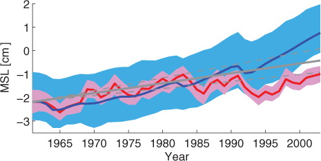
The steric height trend from 1961 to 2003 in FREE is too large compared with the IPCC estimate, although the ensemble envelope overlaps the confidence interval of the observed trend (Fig. 3). On the contrary, the steric height trend in NorCPM is on the low side, albeit the ensemble envelope overlaps the confidence interval of the observed trend. This new validation confirms the conclusion from Wang et al. (2016) that the aggregation method solves the large drift found in Counillon et al. (2014) and produces an acceptable GMSL trend, although it seems to introduce a slight decreasing sea-level drift.

Fig. 3 Estimated global mean sea level (steric) from NorCPM (red), FREE (blue) and observations (plain grey line) for the period the period 1961–2003. The shading represents the ensemble envelope (min and max). The dashed lines represent the 95 % confidence interval of the trend in the observations.

3.3. Altimetry

Spatial variations in SSH on interannual timescale are a measure of dynamically induced density and ocean circulation changes. In regions where the 1.5 layer approximation for the ocean holds (i.e. an active less dense layer over a much thicker and denser inactive layer), then SSH variations are closely related to upper ocean density changes (Wyrtki and Kendall, 1967; Rebert et al., 1985). This relation is strongest in the tropics where the density contrast between the two layers is greatest.

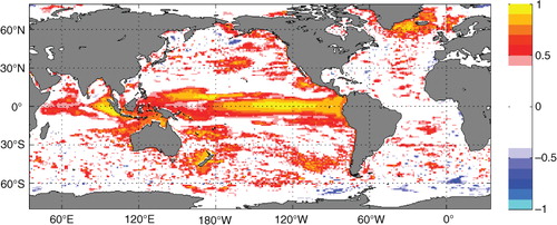
The SSH altimetry data set used for validation is the gridded product from ARMOR3D_REP V3.1 monthly (www.marine.copernicus.eu). It is based on the satellite altimeter data (available from 1993 to present) produced by Ssalto/Duacs and distributed by Aviso with support from the Centre national d’études spatiales (www.aviso.oceanobs.com/duacs/). The product was re-gridded to a 1° resolution in order to have a comparable resolution to the model. Here, we are mainly interested in the capacity of our model to monitor the variability on interannual-to-decadal timescale. We analyse the time variability of the SSH at yearly time scale, and the time series are detrended to remove the long-term trend investigated in Section 3.2. The correlation for FREE is very small and not presented. In Fig. 4, the correlation in NorCPM is very high in the equatorial and in the North Pacific. In the Atlantic, a high correlation is found for the SPG and the Nordic Seas.

Fig. 4 Point-wise correlation of detrended yearly SSH between NorCPM and altimetry data for the period 1993–2010.

3.4. Heat and salt content

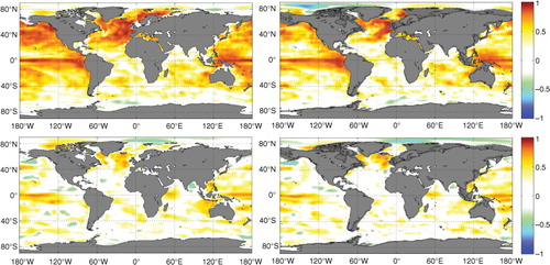
This section investigates the capability of NorCPM to monitor the yearly variability of HC and SC of the top 200 and 500 m. The correlation between the ensemble mean of NorCPM and the objective analysis EN4 (Good et al., 2013, version EN.4.1.1) is shown in Fig. 5. The observations used in EN4 are not assimilated in NorCPM and EN4 can be considered as independent. The correlation is calculated using detrended time series in order to remove the long-term steric change related to the response to the anthropogenic forcing. The correlation for FREE is not shown because it is very low once detrended. In the top 200 m, the correlation for the HC is high in the North Atlantic, the North Pacific and the equatorial Pacific. The correlation remains high for the HC of the top 500 m. There is also some skill in the SC that highlights the multivariate property of our DA method, but the overall skill is weaker than for HC. The regions of higher skill match those of the HC. There are some regions where the correlation is weakly negative, but they should not be over interpreted, as there is a high shortage of salinity observations. For example, the negative correlation pattern in the Arctic seems inconsequential because no observations are available there. Once again, the SPG and the Nordic Sea stand out as regions of higher skill and NorCPM seems capable of monitoring the heat and (to some extent) salt content variability there.

Fig. 5 Point-wise correlation of detrended yearly heat content (upper row) and salt content (lower row) for the period 1950–2010 between NorCPM and EN4 data. The left column is calculated for the top 200 m and the right column is for the top 500 m.

4. The North Atlantic SPG region

The subtropical and the SPG in the North Atlantic work as a mixing battery of warm and saline Subtropical Water, and cold and fresh Subarctic Water, where the characteristic of the waters flowing towards and into the Nordic Seas depends on the relative strength of the two gyres (Hátún et al., 2005). A weakening of the SPG is related to a larger amount of Subtropical Water reaching the Nordic Seas. Furthermore, it has been shown that the characteristics of the waters entering the Nordic Seas over the Greenland–Scotland Ridge are closely related to the strength and width of the SPG, represented by the SPG index. Monitoring and predicting the variability of the SPG have been achieved in state-of-the-art prediction systems (Robson et al., 2012a, 2012b; Yeager et al., 2012; Msadek et al., 2014), but to the best of our knowledge, it has never been achieved with SST only in a real framework. The SPG region stands out in our global validation (HC, SC and SSH) as a region of higher skill. In the following, a deeper investigation is carried out, first using the SPG index and second analysing the vertical temperature anomaly in the SPG region and its connection with the Atlantic Meridional overturning circulation (AMOC).

4.1. The subpolar Gyre index

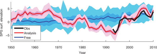
The SPG index is defined as the SSH anomaly in the box (longitude: 15–60°W; latitude 48–65°N), as proposed in the coordinated ocean-ice reference experiments II protocol (Danabasoglu et al., 2014). A strong (weak) SPG – meaning a strong (weak) barotropic SPG mass transport – is characterised by a negative (positive) SPG index. In Fig. 6, we compare the SPG index from NorCPM and FREE with that of the altimetry data available from 1993, that was already used in Section 3.3. FREE shows a slow increase that is associated with the GMSL increase (see Section 3.2). The ensemble spread is large, which indicates that the ensemble samples disparate phases of the SPG. In NorCPM, the ensemble spread is narrower, suggesting that the ensemble members are better synchronised. There is a slight reduction in the ensemble spread with time, which suggests that the synchronisation between members is improving with time possibly because of the improved accuracy of SST with time or due to the cumulative benefit from the assimilation. The ensemble mean in NorCPM shows pronounced phases of positive and negative anomalies, which starts with a weak SPG phase during 1950–1970, followed by a strong SPG phase during the beginning of the 1970s and 1980s. Finally, there is a sharp transition towards a weak SPG around 1995–1996. These phases of the SPG are in good agreement with previous studies (Robson et al., 2012a, 2012b; Yeager et al., 2012; Msadek et al., 2014). The match with the observations in the latter period is striking and it captures not only the shift but also captures the year-to-year variability. The system shows relatively good reliability and the observations fall within the ensemble envelope.

Fig. 6 Subpolar Gyre index in NorCPM (red), FREE (blue) and observations (black line). The darker shading represents the first and third quartile of the model ensemble and the lighter shading represents the ensemble envelope (min/max).

4.2. The stratification of the subpolar Gyre

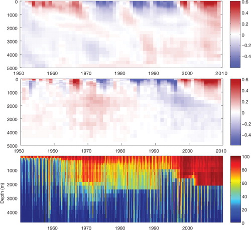
The variability of the SPG is known to be related to the change of its water properties in the thermocline (the upper 1–2 km), which is driven by the convergence of heat (Williams et al., 2014). The evolution of the temperature anomaly in the SPG region is investigated with a Hovmöller plot of the averaged temperature anomaly of the SPG region with respect to the period 1950–2010 (see Fig. 7). The estimate of NorCPM is compared to that of the EN4 objective analysis already used in Section 3.4. The accuracy of the EN4 varies in space and time with the availability of observations. The percentage of available observations is added as an indicator of its accuracy. The temperature anomaly in NorCPM agrees generally well with EN4, in particular at locations where many measurements are available. NorCPM is somewhat smoother, which is expected as the ensemble mean is plotted. The latest transition from a cold and strong SPG (during 1982–1995) to a warm and weak SPG (1996–2009) compares very well with observations in timing, amplitude and depth of the anomaly pattern. Some discrepancies can be noticed below 2000 m where both EN4 and NorCPM become very uncertain. In NorCPM, this is because the influence from SST at such depth is not expected and in EN4 this is because there are almost no observations available below 2000 m. There are also some discrepancies in the upper ocean during the period 1950–1970. While both EN4 and NorCPM indicate that the SPG is anomalously warm during this period, EN4 exhibits a strong vertical stratification not seen in NorCPM. However, this stratification in EN4 may be an artefact of interpolation, as upper ocean observations are scarce during this period, and this type of stratification is not obvious in the later period. Both EN4 and NorCPM suggest a short cold period in the mid-1970s and a warm anomaly around 1980 in relatively good agreements.

Fig. 7 Subpolar Gyre temperature anomaly in NorCPM (top), EN4 (middle) and % of observation used in EN4 analysis (bottom).

4.3. Interaction with the AMOC

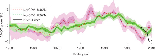
Many studies have identified the interplay between the SPG and the AMOC. Zhang (2008) proposed that the variability in the SPG is a part of a multidecadal variation and that AMOC shows a tight opposite to the SPG. The shift in the 1996 has been attributed to a response to the persistent positive phase of the North Atlantic Oscillation (NAO), which leads to an increase in the AMOC that, in turn, leads to a warming, spin-down and a westward shift of the SPG (Robson et al., 2012a, 2012b; Yeager et al., 2012; Msadek et al., 2014). We consider the maximum monthly poleward transport at 26.5 °N and 45 °N as two indices of AMOC strength (Fig. 8). The average of the AMOC at 26.5 °N in NorESM is 30.8 Sv (1 Sv = 10⁶ m³s⁻¹), which is well above the 17.4 Sv estimate using observations for the year 2004–2011 (Srokosz et al., 2012) and is in the upper range of AMOC strength among models participating in CMIP5 (Reintges et al., 2016). The AMOC is measured continuously from April 2004 at 26.5 °N by a joint US–UK Rapid Climate Change–Meridional Overturning Circulation and Heat flux Array (RAPID–MOCHA; Johns et al., 2011; Smeed et al., 2015). The evolution of the observed AMOC at 26.5 °N is compared with NorCPM (Fig. 8). The overlapping period with our simulation is too short to hold any firm statement, but the preliminary comparison is encouraging with a strong decreasing trend and premise of a rebound at the end of the time series both in NorCPM and in the observations. However, the decreasing trend of the model is too moderate, with a reduction of 2 Sv instead of 4.5 Sv in the observation. Also unlike for the SPG index, the observation does not fall within the ensemble envelope, which indicates that the system lacks reliability. As for the SPG, we can notice that the spread seems to be smaller post 1982, which may indicate that the system is better constrained by the increase in accuracy of the observations associated with the introduction of satellite data.

Fig. 8 AMOC in NorCPM at latitude 45°N (in red) and 26.5°N (in green). The dashed line is the ensemble mean, the dark shading shows the first and third quartile of the ensemble and the light shading shows the ensemble envelope. The black line is the estimate from the RAPID–WATCH array available from 2005 located at 26.5°N. The observed data are adjusted to match the model in 2005.

The variability of the AMOC prior to the observed period is also in relatively good agreement with the literature. The increase of AMOC from the 1970s followed by a subsequent decrease during the 1990s has been reported in several studies (Robson et al., 2012a, 2012b; Yeager et al., 2012; Pohlmann et al., 2013; Karspeck et al., 2015) and is attributed to the response to the long positive NAO. However, there is large uncertainty in AMOC changes in re-analysis, especially in the subtropics (Keenlyside and Ba, 2010; Karspeck et al., 2015). The AMOC variability at 45 °N shows similarities to the one obtained with SST nudging in Swingedouw et al. (2012). In our model, the AMOC at 45°N is tightly connected to the SPG suggesting that the SPG drives the AMOC variability at this latitude (Hátún et al., 2005; Zhang, 2008). There seems to be a relation between the multidecadal variability of AMOC at 26.5 and 45°N with the latter leading the former with a lag of several years, but the period of study is too short. Such mechanism was proposed in Zhang (2010), where the relation between the SPG and the subtropical AMOC is related to the propagation speed of the anomaly in that region. Such relation has been found to vary strongly from model to model (Ba et al., 2014).

4.4. Properties of the covariance: isopycnal and flow dependent

The purpose of this section is twofold: first, it is to identify the impact of constructing the covariance in isopycnal rather than in z coordinates and, second, it is to investigate the flow-dependent properties of our covariance matrix used for DA. This analysis is done for a small box domain in the middle of the Labrador Sea, a region of active wintertime ocean convection that penetrates down to 2000 m and influences the AMOC (Marshall and Schott, 1999; Latif et al., 2006).

The importance of vertical coordinates for the purpose of DA was studied in Gavart and De Mey (1997), who found that isopycnal coordinates are more efficient than z coordinates for capturing the vertical structure of a region in the Azores. Similarly, Srinivasan et al. (2011) found that the performance of DA of an isopycnal model is degraded when the covariance is constructed in z coordinates, rather than in the native isopycnal coordinates. However, the degradation was assumed to be related to information lost by interpolating back and forth between the two vertical coordinate systems. Here, we revisit this issue by comparing the correlation between SST and the vertical profile when the ensemble covariance is constructed in z coordinates versus density coordinates (isopycnal). In Fig. 9, each column corresponds to the ensemble correlation calculated at the time of assimilation (in the middle of the month) during the year 2010. The correlation between SST and isopycnal temperatures, salinities and layer thicknesses are plotted on the left, while on the right the temperature and salinity fields are interpolated to z coordinates for each member prior to the calculation of the correlations. Note that the depth of each isopycnal layer is plotted at the averaged depth of the ensemble mean.

Fig. 9 Hovmöller plot of the ensemble correlation between SST and the water column properties calculated for a box in the centre of the Labrador Sea at the middle of each month in 2010. The correlations on the left are calculated in isopycnal coordinates while those on the right are calculated in z-level coordinates. The upper row is the correlation between SST and temperature, the middle row with salinity and the lower with layer thickness.

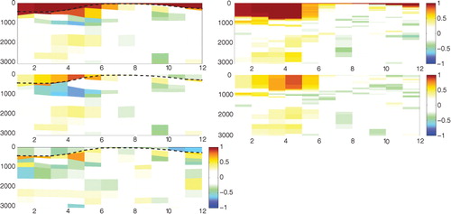
As expected, there is a very high correlation between SST and temperature within the mixed layer and a negative correlation between SST and the layer thicknesses within the mixed layer (Fig. 9). Hence, an increase of SST results in an increase of the stratification and a thinning of the mixed layer. The correlations with the layer thicknesses seem weak but are found to be important. Indeed, an attempt of re-analysis where the layer thicknesses were not updated by assimilation shows a strong degradation in the skill of monitoring the SPG index (not shown). The correlations of SST with salinity within the mixed layer, and with temperature and salinity below the mixed layer are most significant in the late winter. This is consistent with Labrador Sea convection that occurs in late winter when strong heat fluxes cool surface waters, destabilising the water column. During convection, the dense colder and fresher surface water sinks in plumes, while the less dense warmer and more saline Irminger Sea water rises to the surface (Marshall and Schott, 1999). Thus, following deep convection, surface waters will be warmer and more saline and deeper waters will be colder and fresher. This explains why SST is positively correlated with salinity in the climatological mixed layer, and negatively correlated with both temperature and salinity below the mixed layer in the late winter months. Another effect that may enhance the anti-correlation of SST with subsurface salinity in the isopycnal model is the conjugate adjustment of salinity that is necessary to preserve density of isopycnal layers below the mixed layer. The detrainment of surface waters from the mixed layer can introduce long-term predictability, as these properties are ‘stored’ in isopycnal layers. This process is represented well by the isopycnal model.

The correlations in z coordinates are almost identical as when expressed in isopycnal (or density) coordinates within the mixed layer. This is expected because the depth of the mixed layer is almost identical in all members. However, the correlations in late winter with the temperature and salinity below the mixed layer is blurrier and deeper, because the correlation in this depth range considers members that are still in the mixed layer and others that have already transited to isopycnal coordinates. Below 1000 m, the correlation of SST with temperature and salinity does not show the reversal pattern that was seen when constructing the covariance in isopycnal coordinates. At such depth, the position of the isopycnal layers varies and the ensemble formulated in z coordinates combine members with different densities. This can introduce a diffusion of the correlation or even spurious correlation as it increases the risk for non-Gaussian distribution (e.g. bimodality).

Similarly, to what is described in Gavart and De Mey (1997), this comparison highlights the fact that formulating the covariance in z coordinates fails to dissociate the displacement of isopycnal from an anomaly of temperature. A front in SST can have a signature in the position of isopycnal below the thermocline, which implies that DA with a covariance matrix formulated in isopycnal coordinates has the potential to extract more information when assimilating SST than if covariance are constructed in z coordinates. Furthermore, updating the ensemble in z coordinates induces spurious diapycnal mixing. Nevertheless, one drawback of the isopycnal framework is that the combination of water of similar density (with different temperatures and salinities) can introduce artificial caballing, but Counillon and Bertino (2009) and Wang et al. (2016) infer that it is negligible.

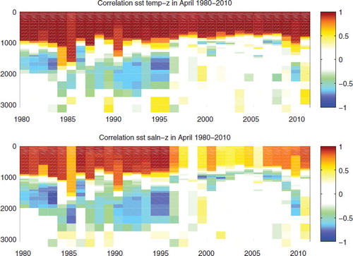
We are analysing the time variability of the dynamical covariance, as it is a singular property of the EnKF DA method. Figure 9 shows a pronounced seasonality in the covariance in the Labrador Sea that demonstrates the need for time-varying covariance. Seasonal covariance can be achieved with computationally ‘cheaper’ DA methods; for example, by using a seasonally varying static ensemble (Xie and Zhu, 2010).

In the Labrador Sea, the covariance of April SST with temperature and salinity over the water column shows pronounced yearly variability (see Fig. 10). This month was selected because it is most related to variations in Labrador Sea water formation, which has been linked to SPG and AMOC variations. The reversal of the correlation at depth observed in 2010 is recurrent in other years, particularly before 1996. While between 1996 and 2008, SST is not correlated with temperature or salinity below the mixed layer. This relation is consistent with observations that show Labrador Sea wintertime deep convection strongly weakened in the mid-1990s, only to resume in 2008 (Våge et al., 2009; van Aken et al., 2011). The variations in Labrador Sea convection have been linked to variations in the SPG and AMOC (Latif et al., 2006; Msadek et al., 2014; Keenlyside et al., 2015).

Fig. 10 Hovmöller plot of the ensemble correlation between SST and the water column properties (upper: temperature; lower: salinity) calculated on the 15th of April of each year between 1980 and 2010.

5. Summary and conclusions

A re-analysis of NorCPM for the period 1950–2010 (doi: 10.11582/2016.00002) is introduced and validated. NorCPM assimilates the stochastic monthly HaISST2 observations with the EnKF into NorESM. The global RMSE for SST anomalies is around 0.4 °C, and there is no clear bias or degradation with time. The signature of the transition of the HadISST2 observation to the satellite era is small. Still, it highlights the challenge of providing consistent re-analysis with a heterogeneous observational network. The system is found overdispersive for SST, particularly before the satellite era. NorCPM shows good spatial reliability for SST, but temporal reliability is poor only capturing the seasonal variability of the RMSE. The steric GMSL rise of the system is on the low side compared with the observed estimate, but it is acceptable. This study further demonstrates that the aggregation method (Wang et al., 2016) can successfully constrain the drift induced by the linear analysis update of the layer thickness.

The system shows good skill against independent data set: SSH, and heat and salt content of the top 200 and 500 m. The benefit is mainly located in the Equatorial and North Pacific, and in the North Atlantic SPG and Nordic Seas. NorCPM demonstrates accurate and reliable skill for monitoring the SPG strength, and it shows some skill for monitoring the vertical evolution of the temperature anomaly in the SPG region. Although the observation period for the AMOC is yet too short, NorCPM shows encouraging results compared with observations and other studies. Prior to the observed period, the anomaly of AMOC and SPG show similarities with other existing re-analysis products (Robson et al., 2012a, 2012b; Swingedouw et al., 2012; Yeager et al., 2012; Pohlmann et al., 2013). Some of the relations between the AMOC and the SPG proposed in the literature are also satisfied in NorCPM: namely, the variability of the SPG index is tightly related to the AMOC at 45°N (Hátún et al., 2005; Zhang, 2008), and the AMOC at 45°N leads the AMOC at 26.5°N by a few years (Zhang, 2010; Ba et al., 2014).

The impact of constructing the covariance in isopycnal coordinates rather than z coordinates and using flow-dependent DA method was studied in the Labrador Sea. Although the current analysis does not demonstrate the necessity of isopycnal flow-dependent covariance, it demonstrates some of its advantages. Expressing the covariance matrix in isopycnal coordinates allows for dissociating the role of anomaly in the water masses on isopycnal surfaces from a displacement of isopycnic surfaces, in good agreement with Gavart and De Mey (1997). As the displacements of isopycnal surfaces have a deep signature, it deepens the impact of assimilation when assimilating surface data. The ensemble covariance in the Labrador Sea shows a strong variability for seasonal and multidecadal time scale; the latter being tightly connected to the SPG shift. This emphasise the benefit of a flow-dependent DA method.

NorCPM achieved some skill by assimilating SST only, which suggests that the system can be used for providing a long re-analysis covering the whole SST observation period (from 1850). However, most of the validation was carried during the later decades at a time when the SST observation is significantly better. It is unclear whether NorCPM would be capable of maintaining comparable level of skill during the whole SST observation period, in particular during the early period when the accuracy of the HadISST2 is significantly poorer. Still, we expect that a full stochastic system (observations and models) such as NorCPM is best suited to handle such a problem, as demonstrated here during the transition to satellite era. The current re-analysis of NorCPM will serve as initial state for climate predictions that will contribute to the CMIP version 6 decadal prediction exercise. Further improvements to the system are ongoing; namely by assimilating other data type (SSH, temperature and salinity hydrographic profiles) or by assimilating in (or across) the other compartments (land, ice and atmosphere).

Finally, the current re-analysis will be used to identify the influence of the ocean variability on the other compartments in a fully coupled framework. The influence of the ocean on the other compartments is occurring dynamically in NorCPM within the monthly assimilation cycle. Comparing the distribution of the relatively large ensemble of NorCPM and FREE can be used to estimate the influence of the ocean on the chaotic behaviour of the atmosphere and the ice compartment.

6. Acknowledgements

This study was partly funded by the Centre for Climate Dynamics at the Bjerknes Centre and the Norwegian Research Council under the NORKLIMA research programme (EPOCASA; 229774/E10), the NordForsk research program ‘Arctic Climate Predictions: Pathways to Resilient, Sustainable Societies’ (ARCPATH, 76654) and the PREFACE project (EU FP7/2007–2013, Grant Agreement No. 603521). This work has also received a grant for computer time from the Norwegian Program for supercomputing (NOTUR2, project no. NN9039K) and a storage grant (NORSTORE, NS9039K). We would like to thank two anonymous reviewers for their valuable comments.

Notes

¹Note that the RMSE is calculated from the monthly averaged model outputs and not from the ensemble of model states at assimilation time (i.e. in the middle of the month). It is thus not ensured that the RMSE is lower than the observation error.

²Some of the correlations for the first layer are undefined because the variance of the ensemble is zero as all members have reached the maximum thickness of 5 m.

References

- Anderson J. L. , Anderson S. L . A Monte Carlo implementation of the nonlinear filtering problem to produce ensemble assimilations and forecasts. Mon. Weather Rev. 1999; 127: 2741–2758.
- Ba J. , Keenlyside N. S. , Latif M. , Park W. , Ding H. , co-authors . A multi-model comparison of Atlantic multidecadal variability. Clim. Dynam. 2014; 43(9–10): 2333–2348.
- Bentsen M., Bethke I., Debernard J. B., Iversen T., Kirkevåg A., co-authors. The Norwegian Earth System Model, NorESM1-M – Part 1: description and basic evaluation. Geosci. Model Dev. Discuss. 2012; 5: 2843–2931. DOI: http://dx.doi.org/10.5194/gmdd-5-2843-2012.
- Bindoff N. L. , Willebrand J. , Artale V. , Cazenave A. , Gregory J. M. , co-authors . Observations: oceanic climate change and sea level. 2007. Changes AR4.
- Bleck R. , Rooth C. , Hu D. , Smith L. T . Salinity-driven thermocline transients in a wind- and thermohaline-forced isopycnic coordinate model of the North Atlantic. J. Phys. Oceanogr. 1992; 22: 1486–1505.
- Bocquet M . Ensemble Kalman filtering without the intrinsic need for inflation. Nonlinear Process. Geophys. 2011; 18(5): 735–750.
- Bocquet M. , Raanes P. , Hannart A . Expanding the validity of the ensemble Kalman filter without the intrinsic need for inflation. Nonlinear Process. Geophys. Discuss. 2015; 2(4): 1091–1136.
- Brune S. , Nerger L. , Baehr J . Assimilation of oceanic observations in a global coupled Earth system model with the SEIK filter. Ocean Model. 2015; 96: 254–264.
- Carton J. A. , Giese B. S . A reanalysis of ocean climate using simple ocean data assimilation (SODA). Mon. Weather Rev. 2008; 136(8): 2999–3017.
- Counillon F. , Bertino L . Ensemble optimal interpolation: multivariate properties in the Gulf of Mexico. Tellus A. 2009; 61(2): 296–308.
- Counillon F., Bethke I., Keenlyside N., Bentsen M., Bertino L., co-authors. Seasonal-to-decadal predictions with the ensemble Kalman filter and the Norwegian Earth System Model: a twin experiment. Tellus A. 2014; 66 21074. DOI: http://dx.doi.org/10.3402/tellusa.v66.21074.
- Craig A. P., Vertenstein M., Jacob R. A new flexible coupler for earth system modeling developed for CCSM4 and CESM1. Int. J. High Perform. Comput. Appl. 2011; 26: 31–42. DOI: http://dx.doi.org/1094342011428141.
- Danabasoglu G. , Yeager S. G. , Bailey D. , Behrens E. , Bentsen M. , co-authors . North Atlantic simulations in coordinated ocean-ice reference experiments phase II (CORE-II). Part I: mean states. Ocean Model. 2014; 73: 76–107.
- Dee D. P . Bias and data assimilation. Q. J. Roy. Meteorol. Soc. 2005; 131(613): 3323–3343.
- Dee D. P. , Uppala S. , Simmons A. , Berrisford P. , Poli P. , co-authors . The era-interim reanalysis: configuration and performance of the data assimilation system. Q. J. Roy. Meteorol. Soc. 2011; 137(656): 553–597.
- Dukowicz J. , Baumgardner J . Incremental remapping as a transport/advection algorithm. J. Comput. Phys. 2000; 160(1): 318–335.
- Evensen G . The ensemble Kalman filter: theoretical formulation and practical implementation. Ocean Dynam. 2003; 53(4): 343–367.
- Evensen G . Data Assimilation: The Ensemble Kalman Filter. 2009; Springer-Verlag Berlin: Springer Science & Business Media.
- Eyring V. , Bony S. , Meehl G. , Senior C. , Stevens B. , co-authors . Overview of the Coupled Model Intercomparison Project Phase 6 (CMIP6) experimental design and organisation. Geosci. Model Dev. Discuss. 2015; 8(12): 10539–10583.
- Ferry N. , Parent L. , Garric G. , Barnier B. , Jourdain N. C . Mercator global eddy permitting ocean reanalysis GLORY S1V1: description and results. Mercator Ocean Q. Newsl. 2010; 36: 15–27.
- Fujii Y. , Kamachi M . Three-dimensional analysis of temperature and salinity in the equatorial Pacific using a variational method with vertical coupled temperature-salinity empirical orthogonal function modes. J. Geophys. Res. Oceans. 2003; 108(C9): 3297.
- Gavart M. , De Mey P . Isopycnal EOFs in the Azores Current region: a statistical tool for dynamical analysis and data assimilation. J. Phys. Oceanogr. 1997; 27(10): 2146–2157.
- Gent P. , Danabasoglu G. , Donner L. , Holland M. , Hunke E. , co-authors . The community climate system model version 4. J. Clim. 2011; 24(19): 4973–4991.
- Good S. A. , Martin M. J. , Rayner N. A . EN4: quality controlled ocean temperature and salinity profiles and monthly objective analyses with uncertainty estimates. J. Geophys. Res. Oceans. 2013; 118(12): 6704–6716.
- Hátún H. , Sandø A. , Drange H. , Hansen B. , Valdimarsson H . Influence of the Atlantic subpolar gyre on the thermohaline circulation. Science. 2005; 309(5742): 1841–1844.
- Holland M. M. , Bailey D. A. , Briegleb B. P. , Light B. , Hunke E . Improved sea ice shortwave radiation physics in CCSM4: the impact of melt ponds and aerosols on Arctic sea ice. J. Clim. 2012; 25(5): 1413–1430.
- Johns W. E. , Baringer M. O. , Beal L. , Cunningham S. , Kanzow T. , co-authors . Continuous, array-based estimates of Atlantic Ocean heat transport at 26.5 N. J. Clim. 2011; 24(10): 2429–2449.
- Kalnay E. , Kanamitsu M. , Kistler R. , Collins W. , Deaven D. , co-authors . The NCEP/NCAR 40-year reanalysis project. Bull. Am. Meteorol. Soc. 1996; 77(3): 437–471.
- Karspeck A., Stammer D., Köhl A., Danabasoglu G., Balmaseda M., co-authors. Comparison of the Atlantic meridional overturning circulation between 1960 and 2007 in six ocean reanalysis products. Clim. Dynam. 2015; 1–26. DOI: http://dx.doi.org/10.1007/s00382-015-2675-1.
- Karspeck A. R. , Yeager S. , Danabasoglu G. , Hoar T. , Collins N. , co-authors . An ensemble adjustment Kalman filter for the CCSM4 ocean component. J. Clim. 2013; 26(19): 7392–7413.
- Keenlyside N. , Latif M. , Botzet M. , Jungclaus J. , Schulzweida U . A coupled method for initializing El Nino southern oscillation forecasts using sea surface temperature. Tellus A. 2005; 57(3): 340–356.
- Keenlyside N. , Latif M. , Jungclaus J. , Kornblueh L. , Roeckner E . Advancing decadal-scale climate prediction in the North Atlantic sector. Nature. 2008; 453(7191): 84–88.
- Keenlyside N. S. , Ba J . Prospects for decadal climate prediction. Wiley Interdiscip. Rev. Clim . Change. 2010; 1(5): 627–635.
- Keenlyside N. S. , Ba J. , Mecking J. , Omrani N.-E. , Latif M. , co-authors . North Atlantic multi-decadal variability-mechanisms and predictability. Climate Change: Multidecadal and Beyond.
- Kirkevåg A. , Iversen T. , Seland Ø. , Hoose C. , Kristjánsson J. , co-authors . Aerosol–climate interactions in the Norwegian Earth System Model–NorESM1-M. Geosci. Model Dev. 2013; 6(1): 207–244.
- Köhl A. , Stammer D . Variability of the meridional overturning in the North Atlantic from the 50-year GECCO state estimation. J. Phys. Oceanogr. 2008; 38(9): 1913–1930.
- Laloyaux P. , Balmaseda M. , Dee D. , Mogensen K. , Janssen P . A coupled data assimilation system for climate reanalysis. Q. J. R. Meteorol. Soc. 2015; 141: 2350–2375.
- Latif M. , Böning C. , Willebrand J. , Biastoch A. , Dengg J. , co-authors . Is the thermohaline circulation changing?. J. Clim. 2006; 19: 4631–4637.
- Lawrence D. M. , Oleson K. W. , Flanner M. G. , Thornton P. E. , Swenson S. C. , co-authors . Parameterization improvements and functional and structural advances in version 4 of the Community Land Model. J. Adv. Model. Earth Syst. 2011; 3(1): 27.
- Lemarié F. , Blayo E. , Debreu L . Analysis of ocean-atmosphere coupling algorithms: consistency and stability. Procedia Comput. Sci. 2015; 51: 2066–2075.
- Marshall J. , Schott F . Open-ocean convection: observations, theory, and models. Rev. Geophys. 1999; 37(1): 1–64.
- McDougall T. J. , Jackett D. R . An assessment of orthobaric density in the global ocean. J. Phys. Oceanogr. 2005; 35(11): 2054–2075.
- Mignot J., García-Serrano J., Swingedouw D., Germe A., Nguyen S., co-authors. Decadal prediction skill in the ocean with surface nudging in the IPSL-CM5A-LR climate model. Clim. Dynam. 2016; 47(3): 1225–1246. DOI: http://dx.doi.org/10.1007/s00382-015-2898-1.
- Mochizuki T. , Masuda S. , Ishikawa Y. , Awaji T . Multiyear climate prediction with initialization based on 4D-Var data assimilation. Geophys. Res. Lett. 2016; 43(8): 3903–3910.
- Msadek R. , Delworth T. , Rosati A. , Anderson W. , Vecchi G. , co-authors . Predicting a decadal shift in North Atlantic climate variability using the GFDL forecast system. J. Clim. 2014; 27(17): 6472–6496.
- Neale R. B. , Chen C.-C. , Gettelman A. , Lauritzen P. H. , Park S. , co-authors . Description of the NCAR Community Atmosphere model (CAM 4.0). 2010. NCAR Tech. Note NCAR/TN-486+ STR.
- Oke P. R. , Sakov P. , Cahill M. L. , Dunn J. R. , Fiedler R. , co-authors . Towards a dynamically balanced eddy-resolving ocean reanalysis: BRAN3. Ocean Model. 2013; 67: 52–70.
- Oleson K. , Lawrence D. , Bonan G. , Flanner M. , Kluzek E. , co-authors . Technical description of version 4.0 of the Community Land Model. 2010; Boulder, CO, USA: National Center for Atmospheric Research. 257. NCAR Tech. Technical Report, Note NCAR/TN-478+STR,.
- Pohlmann H. , Smith D. M. , Balmaseda M. A. , Keenlyside N. S. , Masina S. , co-authors . Predictability of the mid-latitude Atlantic meridional overturning circulation in a multi-model system. Clim. Dynam. 2013; 41(3–4): 775–785.
- Rayner N. , Kennedy J. , Smith R. , Titchner H . 2016. The Met Office Hadley Centre sea ice and sea-surface temperature data set, version 2: 2. Sea-surface temperature analysis (in preparation).
- Rebert J. P. , Donguy J. R. , Eldin G. , Wyrtki K . Relations between sea level, thermocline depth, heat content, and dynamic height in the tropical Pacific Ocean. J. Geophys. Res. Oceans. 1985; 90(C6): 11719–11725.
- Reintges A., Martin T., Latif M., Keenlyside N. S. Uncertainty in twenty-first century projections of the Atlantic meridional overturning circulation in CMIP3 and CMIP5 models. Clim. Dynam. 2016; 1–17. DOI: http://dx.doi.org/10.1007/s00382-016-3180-x.
- Robson J. , Sutton R. , Lohmann K. , Smith D. , Palmer M. D . Causes of the rapid warming of the North Atlantic Ocean in the mid-1990s. J. Clim. 2012a; 25(12): 4116–4134.
- Robson J. , Sutton R. , Smith D . Initialized decadal predictions of the rapid warming of the North Atlantic Ocean in the mid 1990s. Geophys. Res. Lett. 2012b; 39(19): L19713.
- Sadourny R . The dynamics of finite-difference models of the shallow-water equations. J. Atmos. Sci. 1975; 32(4): 680–689.
- Saha S. , Moorthi S. , Pan H.-L. , Wu X. , Wang J. , co-authors . The NCEP climate forecast system reanalysis. Bull. Am. Meteorol. Soc. 2010; 91(8): 1015–1057.
- Sakov P. , Counillon F. , Bertino L. , Lisæter K. , Oke P. , co-authors . TOPAZ4: an ocean-sea ice data assimilation system for the North Atlantic and Arctic. Ocean Sci. 2012; 8: 633–656.
- Sakov P. , Oke P . A deterministic formulation of the ensemble Kalman filter: an alternative to ensemble square root filters. Tellus A. 2008; 60(2): 361–371.
- Sakov P. , Sandery P. A . Comparison of EnOI and EnKF regional ocean reanalysis systems. Ocean Model. 2015; 89: 45–60.
- Smeed D., McCarthy G., Rayner D., Moat B., Johns W., co-authors. Atlantic Meridional Overturning Circulation Observed by the RAPID-MOCHA-WBTS (RAPID-Meridional Overturning Circulation and Heatflux Array-Western Boundary Time Series) Array at 26N from 2004 to 2014. 2015; Brownlow St, UK: British Oceanographic Data Centre – Natural Environment Research Council. DOI: http://dx.doi.org/10.5285/35784047-9b82-2160-e053-6c86abc0c91b.
- Srinivasan A. , Chassignet E. , Bertino L. , Brankart J. , Brasseur P. , co-authors . A comparison of sequential assimilation schemes for ocean prediction with the HYbrid Coordinate Ocean Model (HYCOM): twin experiments with static forecast error covariances. Ocean Model. 2011; 37(3): 85–111.
- Srokosz M. , Baringer M. , Bryden H. , Cunningham S. , Delworth T. , co-authors . Past, present, and future changes in the Atlantic meridional overturning circulation. Bull. Am. Meteorol. Soc. 2012; 93(11): 1663–1676.
- Storto A., Masina S., Navarra A. Evaluation of the CMCC eddy-permitting global ocean physical reanalysis system (C-GLORS, 1982–2012) and its assimilation components. Q. J. Roy. Meteorol. Soc. 2016; 142(695): 738–758. DOI: http://dx.doi.org/10.1002/qj.2673.
- Swingedouw D., Mignot J., Labetoulle S., Guilyardi E., Madec G. Initialisation and predictability of the AMOC over the last 50 years in a climate model. Clim. Dynam. 2013; 40(9–10): 2381–2399. DOI: http://dx.doi.org/10.1002/qj.2673.
- Titchner H. A. , Rayner N. A . The Met Office Hadley Centre sea ice and sea surface temperature data set, version 2: 1. Sea ice concentrations. J. Geophys. Res. Atmos. 2014; 119(6): 2864–2889.
- Tjiputra J. , Roelandt C. , Bentsen M. , Lawrence D. , Lorentzen T. , co-authors . Evaluation of the carbon cycle components in the Norwegian Earth System Model (NorESM). Geosci. Model Dev. 2013; 6(2): 301–325.
- van Aken H. M. , De Jong M. F. , Yashayaev I . Decadal and multi-decadal variability of Labrador Sea Water in the north-western North Atlantic Ocean derived from tracer distributions: heat budget, ventilation, and advection. Deep Sea Res. Part I Oceanogr. Res. Pap. 2011; 58(5): 505–523.
- Våge K. , Pickart R. S. , Thierry V. , Reverdin G. , Lee C. M. , co-authors . Surprising return of deep convection to the subpolar North Atlantic Ocean in winter 2007–2008. Nat. Geosci. 2009; 2(1): 67–72.
- Vertenstein M., Craig T., Middleton A., Feddema D., Fischer C. CESM1.0.3 user guide. 2012. Online at: http://www.cesm.ucar.edu modelscesm1.0cesmcesm_doc_1_0_3ug.pdf.
- Wang Y. , Counillon F. , Bertino L . Alleviating the bias induced by the linear analysis update with an isopycnal ocean model. Q. J. Roy. Meteorol. Soc. 2016; 142: 1064–1074.
- Weber R. J. , Carrassi A. , Doblas-Reyes F. J . Linking the anomaly initialization approach to the mapping paradigm: a proof-of-concept study. Mon. Weather Rev. 2015; 143: 4695–4713.
- Williams R. G. , Roussenov V. , Smith D. , Lozier M. S . Decadal evolution of ocean thermal anomalies in the North Atlantic: the effects of Ekman, overturning, and horizontal transport. J. Clim. 2014; 27(2): 698–719.
- Wyrtki K. , Kendall R . Transports of the Pacific equatorial countercurrent. J. Geophys. Res. 1967; 72(8): 2073–2076.
- Xie J. , Zhu J . Ensemble optimal interpolation schemes for assimilating Argo profiles into a hybrid coordinate ocean model. Ocean Model. 2010; 33(3): 283–298.
- Yeager S. , Karspeck A. , Danabasoglu G. , Tribbia J. , Teng H . A decadal prediction case study: late twentieth-century North Atlantic Ocean heat content. J. Clim. 2012; 25(15): 5173–5189.
- Zhang R . Coherent surface-subsurface fingerprint of the Atlantic meridional overturning circulation. Geophys. Res. Lett. 2008; 35(20): L20705.
- Zhang R . Latitudinal dependence of Atlantic meridional overturning circulation (AMOC) variations. Geophys. Res. Lett. 2010; 37(16): L16703.
- Zhang S. , Anderson J. , Rosati A. , Harrison M. , Khare S. P. , co-authors . Multiple time level adjustment for data assimilation. Tellus A. 2004; 56(1): 2–15.
- Zhang S. , Harrison M. , Rosati A. , Wittenberg A . System design and evaluation of coupled ensemble data assimilation for global oceanic climate studies. Mon. Weather Rev. 2007; 135(10): 3541–3564.
- Zhang S. , Rosati A. , Delworth T . The adequacy of observing systems in monitoring the Atlantic meridional overturning circulation and North Atlantic climate. J. Clim. 2010; 23(19): 5311–5324.
- Zuo H., Balmaseda M. A., Mogensen K. The new eddy-permitting orap5 ocean reanalysis: description, evaluation and uncertainties in climate signals. Clim. Dynam. 2015; 1–21.. doi: http://dx.doi.org/10.1007/s00382-015-2675-1.