Multiple equilibria on planet Dune: climate–vegetation dynamics on a sandy planet

ABSTRACT

We study the interaction between climate and vegetation on an ideal water-limited planet, focussing on the influence of vegetation on the global water cycle. We introduce a simple mechanistic box model consisting in a two-layer representation of the atmosphere and a two-layer soil scheme. The model includes the dynamics of vegetation cover, and the main physical processes of energy and water exchange among the different components. With a realistic choice of parameters, this model displays three stable equilibria, depending on the initial conditions of soil water and vegetation cover. The system reaches a hot and dry state for low values of initial water content and/or vegetation cover, while we observe a wet, vegetated state with mild surface temperature when the system starts from larger initial values of both variables. The third state is a cold desert, where plants transfer enough water to the atmosphere to start a weaker, evaporation-dominated water cycle before they wilt. These results indicate that in this system vegetation plays a central role in transferring water from the soil to the atmosphere and trigger a hydrologic cycle. The model adopted here can also be used to conceptually illustrate processes and feedbacks affecting the water cycle in water-limited continental areas on Earth. †Now at: International Max Planck Research School on Earth System Modelling, Hamburg, Germany

• climate–vegetation interactions
• multiple stable states
• water cycle
• zero-dimensional models
• evapotranspiration

1. Introduction

The climate and the biosphere of the Earth interact with each other in multiple, complex ways on many spatial and temporal scales. Climate dynamics and variability affect the functioning of individual organisms and ecosystems, which in turn feed back on the climate system, controlling crucial processes such as albedo changes, water and carbon fluxes, or aerosol production (see e.g. Adams et al., 2008; Rietkerk et al., 2011, and references therein).

In fact, the links between the biosphere and the climate of the Earth are so strong that some researchers have proposed that living organisms are the main determinants of global climate as we know it (Vernadsky, 1926; Lovelock, 1986, 1989). This issue has become even more pertinent after the discovery of hundreds of extra-solar planets, and the associated quest for possible evidences of alien life forms (Lovelock, 1965; Spiegel et al., 2008), which underline that the likelihood of desert planets orbiting around a star with energy properties compatible with life existence is concrete and non-fictional.

Simple mathematical models can be useful for studying some of the climate-biosphere interaction processes, such as the effects of vegetation on albedo (Brovkin et al., 1998), or on water fluxes in arid environments (e.g. Zeng, 1999; Baudena et al., 2008). On a global scale, the ‘parable of Daisyworld’ by Watson and Lovelock (1983) is one of the clearest examples of a simple description aimed at capturing the workings of the Earth biosphere (see also the review of Wood et al., 2008). Conceptual models of this kind do not provide quantitative descriptions of climate-biosphere interactions, but rather attempt at exploring avenues and mechanisms that can play a role in the real system, providing inspiration for further research.

In this spirit, we develop here a simple conceptual box model, to explore whether and how vegetation affects the planetary hydrologic cycle. We imagine a planet with no oceans and whose surface is entirely covered with sand (somewhat similar to planet Dune-Arrakis of the sciencefiction book series by Frank Herbert, 1965). We suppose that water can be either in the soil, below the surface, or in the atmosphere, in liquid or vapour forms. Without vegetation, only evaporation can transfer water from the soil surface to the atmosphere, affecting only a thin surface soil layer. What happens to this planet when vegetation is introduced? The roots can reach the soil water contained in deeper soil layers, and plant transpiration can transfer much larger amounts of water to the atmosphere. Is the presence of vegetation sufficient to trigger a hydrologic cycle, leading to enough precipitation to sustain the vegetation itself? If this is the case, what is the minimum vegetation cover that is required to maintain the cycle active? In more precise terms, does the introduction of vegetation lead to multiple equilibria (or solutions) in the soil–vegetation–atmosphere system? Two well-known physical feedback mechanisms may indeed generate multi-stability (e.g. Brovkin et al., 1998; Dekker et al., 2007; Baudena et al., 2008; Janssen et al., 2008). One feedback is associated with the fact that vegetated surfaces have lower albedo than bare ones. As a consequence, soil surface temperature increases, leading to larger atmospheric instability and thus to larger precipitation, favouring vegetation through increased soil water availability (Charney, 1975). The second feedback is connected to plant transpiration being larger than simple evaporation from bare soil. Larger atmospheric humidity increases precipitation, and thus vegetation favours its own growth (e.g. Zeng, 1999).

Although the box model introduced here is best formulated in terms of a hypothetical sandy planet, the results can also provide a conceptual description of the land-atmosphere interaction on wide continental regions of the Earth. Globally, the largest fraction of atmospheric moisture comes from evaporation from the ocean surface. However, over continents 10 to 55% of the water in the atmosphere comes from evapotranspiration (Joussaume et al., 1986; Brubaker et al., 1993). With the help of global circulation models, more recent studies have analysed the effects of land-atmosphere coupling, and the influences of land surface within the hydrologic cycle on Earth (e.g. Fraedrich et al., 2005; Goessling and Reick, 2011). The model discussed here can illustrate the role of vegetation on these continental areas, when discarding the moisture influx from the ocean.

2. Model description

We adopt a box model that describes the dynamics of the spatially-averaged temperature and moisture content on the whole planet (or in a large continental area with negligible moisture input from the ocean), following an approach similar to that of D'Andrea et al. (2006) and Baudena et al. (2008). We divide the soil-atmosphere box vertically into four layers, representing respectively the free troposphere, the planetary boundary layer (PBL), the planetary surface soil and a deeper soil layer (see Fig. 1 for a schematic representation of the model structure). Vegetation grows on the soil surface, but its roots dig deep into the soil.

Fig. 1.  Schematics of the model structure, and list of model variables.

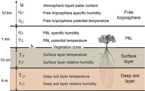
In each layer, we define two dynamical variables, temperature and humidity, each with its own prognostic equation. We simulate vegetation dynamics by including an equation for the fraction of the planet surface covered with vegetation, and explicitly model the variations of the atmospheric liquid water content in the free troposphere. This provides a total of 10 dynamical (prognostic) variables in the model system. The equations account for the water cycle, with its atmospheric and terrestrial branches, the energy balance, and the growth and retreat of vegetation cover. Figure 1 includes a list of the prognostic variables.

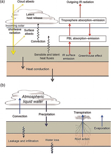
The energy exchanges in the model are schematically represented in Fig. 2a. The radiation coming from the local star (which we will anyway call solar radiation for simplicity) is partially reflected by clouds and by the planet surface owing to the planetary albedo. The ground absorbs the radiation that is not reflected, and thus the soil heats up. The surface reemits part of the energy received as infrared radiation, which is then transferred through the two atmospheric layers. Part of the energy is transferred by conduction deeper into the soil. We model the sensible heat flux between the surface and the PBL, and the convective flux between the PBL and the troposphere. Latent heat exchanges cool the soil surface, because of evapotranspiration, and heat the upper troposphere in case of cloud formation. Water exchanges are represented in Fig. 2b. The root action transfers water from the deep soil layer into the PBL, and evaporation takes place from the surface layer. In the troposphere, part of the water condensates into clouds and precipitates as rain. Rainfall water penetrates in the soil as a consequence of percolation and infiltration processes, and may be lost below the root layer. The convective mass flux transports PBL moisture into the free troposphere. Convection dries and cools the PBL, moisturising and heating the free troposphere. The convective stability of the atmospheric column is defined by the values of the moist enthalpies in the PBL and in the free troposphere (see Section 2.3 for a complete description of the convection parameterisation). In the model formulation, we did not include the seasonal dependence of the integrated stellar radiation reaching the planet, which is rather limited when integrated over the whole planetary surface in the case of weakly elliptical planetary orbits (recall that this is a zero-dimensional box model representing the entire planet). If the model were extended to include latitude dependence, the seasonal modulation of incoming radiation should be taken into account. We also did not include solid precipitation, and the possible formation of polar ice caps is ignored. Overall, the model is meant for a relatively warm and arid planet.

Fig. 2.  Panel (a) shows a scheme of the energy balance: incoming solar radiation travels through the atmosphere, which is transparent to short-wave radiation, but a part of it is reflected by clouds. Surface heating depends on the surface albedo, which is a function of vegetation cover. The surface layer emits long-wave (infrared) radiation upwards. Arrows in the atmosphere show absorption/emission of thermal radiation by the different layers. Panel (b) shows a scheme of the water cycle. Water vapour in the PBL is uplifted by convective fluxes. Water then may condensate in the free troposphere and precipitate as rainfall. Evapotranspiration has the essential role of transferring water back into the atmosphere. Without this effect, the deep soil reservoir would not take part in the cycle, and after some losses water would remain stored there.

In the following, we separately describe the atmospheric dynamics (Section 2.1) and the soil–vegetation dynamics (Section 2.2). We describe in deeper detail the convection scheme and the representation of precipitation formation (Section 2.3 and Section 2.4 respectively).

2.1. Atmosphere

We assume that the atmosphere of this hypothetical planet has similar characteristics to the terrestrial atmosphere. We divide the atmospheric column into the PBL (0≤z≤1000 m) and the free troposphere (1000<z≤11 000 m). We assume the atmosphere to be completely transparent to incoming solar short-wave radiation, with the only exception of cloud albedo. On the other hand, the atmosphere is not fully transparent to infrared radiation, i.e. greenhouse effect is included. The equations describing atmospheric dynamics are:1 2 3 4 5

The terms with indicate instantaneous adjustments of the related quantities, i.e adjustment performed within one time step δt (in the following, δt=1 hour). Equations (1) and (2) provide the tendencies for the temperatures of the free troposphere (U) and the PBL (L), respectively. Equations (3) and (4) describe the dynamics of atmospheric moisture, while the dynamics of the atmospheric liquid water content is described by eq. (5). See Table 1 for a list of the symbols used and the values of the corresponding quantities.

Table 1. Parameter names, symbols, values and unit of measurements

Symbol	Meaning	Value	Unit
Le	Specific latent heat of evaporation	2.501·10^6	J kg^−1
cp	Air specific heat	1000	J kg^−1 K^−1
cps	Soil specific heat	1000	kg m^−3
ρ U	Air density in the upper atmospheric layer	0.720	kg m^−3
ρ L	Air density of PBL	1.200	kg m^−3
ρ W	Water density	1000	kg m^−3
ρ s	Soil density	1800	kg m^−3
hU	Thickness of upper atmospheric layer	10000	m
hL	Thickness of PBL	1000	m
ZT	Depth of surface soil layer	0.1	m
ZD	Depth of deep soil layer	4.0	m
Z 0	Depth of bottom soil layer	10.0	m
n	Soil porosity	0.4
W 0	Maximum water content in the atmosphere before precipitation	5.0	kg m^−2
β	Ratio between sensible and latent convective heat flux	2
ɛ U	Free troposphere absorption/emission coefficient	0.25
ɛ L	PBL absorption/emission coefficient	0.22
ɛ W	Liquid water absorption/emission coefficient	0.6
ɛ S	Soil absorption/emission coefficient	0.85
α e	Albedo of bare soil	0.25
α v	Albedo of vegetated soil	0.18
S	Shading effect coefficient	0.5
	Timescale for temperature relaxation between surface and deep soil layer	180	d
	Timescale for temperature relaxation between deep soil layer and the soil below	360	d

The potential temperature in the upper troposphere, θ _U [eq. (1)], increases owing to the heat received from the ground, in the form of latent heat released by condensation (1st term on the r.h.s.) and convective sensible heat flux (2nd term on the r.h.s., see description below). The upper troposphere exchanges infrared radiation with the soil (3rd term on the r.h.s.), the PBL (4th and 5th term) and outer space (6th term).

The potential temperature in the PBL, θ _L [eq. (2)], varies owing to sensible heat flux from the ground, Q _s [1st term on the r.h.s., see also eq. (2) in Appendix], convective cooling (2nd term), infrared radiation emitted by the ground (3rd term) and the free troposphere (4th term). The last term on the r.h.s. represents infrared emission from the PBL.

In eq (1) and (2), the emission temperatures used in the radiative terms are obtained from the potential temperatures, assuming reference pressure levels within the atmospheric layers (960 and 700 hPa for the PBL and for the free troposphere respectively). The atmospheric layers emit both upwards and downwards, as illustrated in Fig. 2a. The upper troposphere absorbs part of the infrared radiation emitted by the PBL. The part that is not absorbed is lost to space, as well as half of the radiation emitted by the free troposphere. Absorption and emission of radiation take into account the possible presence of liquid water W, distinguishing absorption/emission coefficients between dry and wet emissivities. The constant W ₀ is a normalisation term, indicating the maximum amount of liquid water that can be hold in clouds before it precipitates.

The dynamics of specific humidity in the upper layer, q _U [eq. (3)], includes a source term , representing the convective moisture updraft from the PBL, and a loss term δW, i.e. the amount of water vapour that condensates at each time step.

The dynamics of atmospheric moisture in the PBL, q _L [eq. (3)], is driven by soil evaporation E and plant transpiration R, which occur respectively in the bare soil, covering a fraction 1−b of the total surface, and in vegetated soil, covering a fraction b of the surface (1st and 2nd terms on the r.h.s.). We define the evapotranspiration parameterisation as in Baudena and Provenzale (2008) (for more details, see Section 2.2 and the Appendix).

We assume that liquid water is present only in the free troposphere, above the PBL (i.e. we discard the liquid water content in the PBL). Equation (5) represents the dynamics of the atmospheric liquid water content W in the upper layer. The source term is condensation, as in eq. (3), and the loss term is precipitation P.

We define the amount of water vapour which condensates at each time step as:6

Here q _sat is the specific humidity of saturation, which depends on the tropospheric physical temperature T _U , and is calculated through the Clausius-Clapeyron relation at the fixed reference pressure of 700 hPa.

2.2. Soil and vegetation

Soil dynamics has different timescales with respect to the atmosphere. In general, the soil response to forcing takes longer to become significant, because of the different thermal capacity. As a consequence, the slower soil dynamics asymptotically dominates the whole system dynamics. In addition, part of the soil surface can be vegetated, and vegetation responds significantly more slowly than the atmosphere. In our model, the dynamics of vegetation and soil are strongly interconnected. Evapotranspiration depends on vegetation cover, and vegetation growth and mortality depend on the soil moisture content.

We divide the soil into two layers: The surface layer is the upper part of the soil, with depth Z _T =10 cm, where evaporation takes place. The deep soil layer is thicker, with depth Z _D =4 m, and it acts as a water reservoir. The state variables used for the soil are soil temperature (T _T and T _D for the surface and deep layer respectively) and relative soil moisture, s _T and s _D respectively, with 0<s<1.

The corresponding prognostic equations are:7 8 9 10 11

The dynamics of surface temperature [eq. (7)] is determined by the incoming solar radiation F_rad , which is partly reflected owing to the albedo of bare (α _e ) and vegetated (α _v ) soil. Incoming solar radiation depends also on the atmospheric liquid water content W, since part of the radiation is scattered at the top of the atmosphere by clouds. The quantity Q _s is sensible heat flux, as in eq. (4), while the 3rd, 4th and 5th terms on the r.h.s. represent respectively infrared emission from the surface layer, absorption of infrared radiation re-emitted by the PBL, and absorption of infrared radiation re-emitted by the upper troposphere. The last two terms on the r.h.s. are the latent heat fluxes L _e E and L _e R, which depend on evaporation and transpiration [see also eq. (9) below, and eq. (3) and (4) in the online Appendix]. Evaporation is reduced by a factor S in vegetated areas b, representing plant shading effect, while transpiration does not occur in bare soil. Finally, the last term represents a conductive relaxation to the deep soil temperature T _D .

The equation for the deep soil temperature includes only conductive relaxation [eq. (8)]. The 1st term on the r.h.s. represents relaxation to the surface temperature [same term as in eq. (7)], while the second term is a relaxation to a fixed reference temperature T ₀, representing the temperature of a deeper soil layer which does not participate in the vegetation dynamics (i.e. the soil layer below the deepest plant roots).

Relative soil moisture of the top soil layer, s _T , increases because of precipitation P, and decreases because of evaporation E, leakage L and deep infiltration δI [eq. (9)]. Evapotranspiration is a non-linear function of s _T (see eq. (7) above and eq. (3) in the Appendix). We did not include the contributions of runoff (surface or baseflow) or lateral ground flow, as the model formulation adopted here is spatially implicit (i.e. there is no dependence on the spatial coordinates).

Leakage losses represent an imbalance between gravity and the water holding capacity of the soil, occurring when the soil is close to saturation and water percolates to lower soil layers [eq. (5) in the Appendix]. As such, it is not an instantaneous process. On the other hand, deep infiltration is a very fast process, occurring immediately after a rainfall event. In case of large rainfall events, the soil saturates, and all water in excess is assumed to be instantaneously removed and transferred to the deeper layers [eq. (6) in Appendix, see also Laio, 2001; Baudena and Provenzale, 2008]. We do not represent transpiration losses from the thin surface layer, because we assume root density at the soil surface to be negligible (see Baudena and Provenzale, 2008).

Similar terms can be found in eq. (10), describing moisture dynamics in the deep soil. Deep soil water can be extracted by transpiration in vegetated areas (3rd term on the r.h.s.), which grows non-linearly with s _D [see eq. (7) above and eq. (4) in the Appendix].

In the deep soil layer, water can percolate or infiltrate to an even deeper layer which cannot be reached by the plant roots, and it is lost to the system. These water losses are described by the last two terms in eq. (10), and are discussed in deeper detail in the supplementary material. Owing to the presence of water losses, a self-sustained hydrologic cycle can be generated only if enough water circulates between the plants, the atmosphere and the soil layers reached by the plant roots. The common threshold form for the leakage adopted here allows this cycle to be established and maintained if soil moisture in the lower soil layer does not exceed the hydraulic conductivity. Note, also, that we tested different parameterisation of leakage and different parameter values, finding that the qualitative behaviour of the model did not change.

Equation (11) describes the dynamics of vegetation cover, with a standard logistic equation for the fraction of surface covered with vegetation, b, encompassing a colonisation and a local extinction (mortality) term (Tilman, 1994; Baudena et al., 2007). We assume that the local vegetation mortality µ depends on the deep soil moisture, where roots uptake water and nutrients. The colonisation rate g is a strongly non-linear function of the soil moisture in both layers [see eq. (7) in the Appendix].

2.3. Convection parameterisation

Atmospheric convection is a fundamental process in the model, and it occurs when the atmospheric column becomes unstable. Following D'Andrea et al. (2006) we choose a stability criterion based on the equivalent potential temperature. The equivalent potential temperature of the PBL, θ _e,L , and of the free troposphere, θ _e,U , are defined as:12

where θ is the potential temperature and q is the specific humidity in each layer. When the equivalent potential temperature of the PBL becomes larger than that of the troposphere, the column becomes unstable and convection ensues.

Convection transfers heat and moisture from the PBL to the free troposphere. This is represented by the terms and , which appear in the source terms of eq. (1) and (3), and in the sink terms of eq. (2) and (4). and are finite quantities of heat and humidity that are transferred between the layers, the transfer taking place instantaneously, or, more precisely, in one time-step δt. To compute these terms, we impose convective adjustment; after the convective process, θ _e,L =θ _e,U , which gives:13

As a consequence of convection and the associated sensible and latent heat fluxes, the PBL gets dryer and cooler, the free troposphere becomes warmer and moister, and the atmospheric column (temporarily) stabilises.

To define in what proportion sensible and latent heat fluxes contribute to the adjustment, here we impose a fixed ratio, β (somewhat analogous to the Bowen ratio, Bowen, 1926):14

Hence, eq. (13) and (14) allow computing of the two unknown quantities and .

The quantity β is a free parameter of the system. Physically, there is a lower threshold to β: in our case, for β≤ 0.1, water is lost during the convection process as not enough water is transferred from the PBL to the upper atmospheric layer. Thus, to comply with water conservation we need to fix β>0.1. On Earth, the value of β depends on the type of surface, and it is heavily affected by the presence of surface water bodies. Above deserts, this ratio can reach very high values, up to 10–20. In the current situation, we choose β=2, a value which is in the range appropriate for arid or semi-arid conditions (see, e.g. Chapin III et al., 2011, and references therein).

2.4. Precipitation

In the model, precipitation originates only from the free troposphere above the PBL. Here, if specific humidity exceeds saturation, it condensates into liquid water, releasing latent heat. Droplets may either float in the atmosphere (clouds) or precipitate as rainfall. Precipitation (in kg m⁻²s⁻¹) is estimated instantaneously (i.e. within one time-step) as a fraction of the total liquid water:15

The fraction of liquid water that precipitates is given by the sum of the two terms f _c and f _W . These correspond to the two mechanisms of rain formation that constitute our very coarse parameterisation of cloud microphysics. In detail:

• f _c parameterises the collisions induced by strong convective mass fluxes. It measures the efficiency of moist convection in generating immediate precipitation, and it is a function of the intensity of convection as in D'Andrea et al. (2006), see also eq. (10) in the Appendix.

• f _W parameterises the collision probability leading to droplet coalescence and to the growth of raindrops, and it depends on the square of droplet concentration as in simple two-body collision processes. The larger the concentration of droplets, the more likely collisions become, generating larger drops and thus precipitation. We assume , where W ₀ is the column-integrated droplet density corresponding to the maximum collision efficiency (f _W =1), i.e. when all water droplets are transformed into raindrops in one time step.

These two terms can be seen as the parameterisation of the precipitation due to storms and intense convection (f _c ) and of the precipitation due to large-scale condensation (f _W ). In a very crude sense, f _c is associated with convective precipitation and f _W to stratiform precipitation.

3. Multiple equilibria in the climate–vegetation system

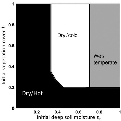
The numerical investigation of the model described above indicates that, in a realistic parameter range, the system displays three co-existing stable states, and no periodic or chaotic dynamics was detected. In the following, we shall always start the model without water in the surface soil layer, and with very little humidity in the atmosphere. The deep soil layer is thus the main water reservoir.

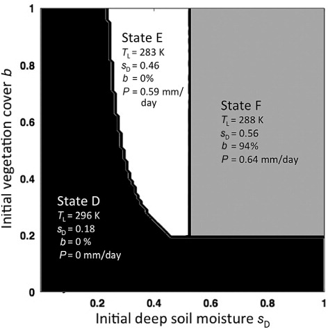
We vary the initial conditions of deep soil moisture and vegetation cover within their whole range (between 0 and 1), and we run the model until an equilibrium state is attained (Fig. 3). The three co-existing stable states are: (1) a hot desert state (hereafter referred to as ), when starting from very dry and/or very low vegetation conditions; (2) a temperate, vegetated state (F), reached when the initial value of s _D is quite high () and vegetation is initially present (); (3) a cold desert (, standing for ‘evaporative desert’). The values of the main variables in each state are summarised in Fig. 3.

Fig. 3.  Equilibrium potential temperature in the PBL for the parameter values indicated in the Appendix, as a function of the initial conditions on s _D (x-axis) and on b (y-axis). The black area indicates the equilibrium state (dry and hot, ), the white area indicates state (dry and cold, ), and the grey area indicate state (wet and temperate, ).

The state is a desert world, in which the planet does not have any vegetation. The initial vegetation cover and total water amount are insufficient to start a water cycle. In this state, there is no liquid water in the atmosphere, thus no precipitation is observed. Surface temperature is about 23°C, soil moisture is very low and latent heat fluxes are almost zero.

The state is observed when the initial conditions of deep soil moisture are high, and vegetation cover is large enough. At equilibrium, a large fraction of the planet surface is covered with vegetation. Owing to the high soil moisture, latent heat fluxes are strong enough to overcome the warming effect of the albedo feedback (Charney, 1975), and the surface temperature (about 15°C) is lower than in the hot desert state .

The third state, , is also a desert world, but with cooler conditions (about 10°C). The total amount of water available in the system is not enough to allow vegetation growth at equilibrium. Nevertheless, there is a transient phase at the beginning of the simulation where vegetation persists long enough to pump a sufficient amount of water into the atmosphere. A weak, evaporation-driven water cycle is started and continues to exist at equilibrium. Precipitation evaporates from the surface soil, leading to latent heat fluxes that cool the soil and the PBL. The long transient phase is due to the positive feedback between vegetation and rainfall. 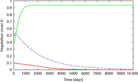In this case, the evapotranspiration feedback is not strong enough to push the system to the state. Nevertheless, it lowers the mortality rate of vegetation, slowing down the extinction process, and injecting enough water in the atmosphere. The transient behaviour of the system is illustrated in Fig. 4, where the vegetation cover b is plotted for the first 10 000 d of integration. We show three integrations where the system is initialised differently, which leads to the three stable states.

Fig. 4.  Temporal dynamics of vegetation cover, starting from different initial conditions of deep soil moisture s _D and vegetation cover b, and reaching three different states: (red dashed line), (green continuous line), and (blue dotted line). Note the different timescales needed to reach the various states. In these simulations, initial conditions used to reach state are s _Di =0.6, and b _i =0.1; state , s _Di =0.5, and b _i =0.5; state , s _Di =0.6, and b _i =0.4.

Convection is active in states and . The state is colder and drier than the state, but it remains convectively unstable because the difference in equivalent potential temperature between the PBL and the free troposphere is positive. The difference in precipitation in the two states is due to a higher amount of large-scale condensation in the state, due to a much higher amount of liquid water (cloud cover).

These results are obtained according to a particular choice of parameters, hereinafter called SC (standard configuration; see Table 1). Soil parameters correspond to sandy loam soil. References for parameter values are Laio (2001); Kållberg et al. (2005); D'Andrea et al. (2006); Baudena et al. (2008); Baudena and Provenzale (2008) and references therein.

Values of equivalent potential temperature are in keeping with the ones found on Earth. Values in states and , in particular, resemble equivalent potential temperatures in subtropical an equatorial regions respectively.

3.1. Model sensitivity to changes in parameter values

We performed several model simulations to determine model sensitivity to parameter variations.

The model is rather insensitive to the values of some parameters. Soil type is one of them, as we verified by changing the soil to loamy sand, analogously, changing the value of the wilting point does not change the qualitative behaviour of the model. We also verified that the model is rather insensitive to considering plant wilting point and soil hygroscopic point (i.e. the minimum soil moisture below which evaporation does not take place) as coincidental. Although these two soil moisture values can differ by a factor of 10 (e.g. Mahfouf, 1991), in the model formulation for simplicity we followed Rodriguez-Iturbe (2000), and we used only one and the same value for the two points. In fact, the contribution of the soil to the evaporation fluxes between hygroscopic point and wilting point is in general very small, and thus negligible for the goal of the present study (note that in the model evaporation grows linearly with soil water content).

For other parameters, the situation is more complex and it is discussed below. In the following, we discuss the results obtained by varying the albedo coefficients, the convective adjustment ratio β, the solar constant and the soil and root depths.

On Earth, the surface albedo varies significantly between deserts, vegetated areas, glaciers, and oceans. In this model we consider only two values for the surface albedo, α _e for bare soil and α _v for vegetated soil. Even though the albedo influences surface temperatures, its role in the model is not crucial for determining the existence, the stability and the basin of attraction of the equilibrium states. The system behaviour does not qualitatively change even when shutting off the albedo effect (i.e. setting α _e =α _v ), or increasing the difference between the two values ().

The value of β is a free parameter of the model, and we use it to determine convective adjustment explicitly. We tune its value in order not to lose or create water during convective events. To assess the model sensitivity to this parameter, we changed β from a half to twice its SC value (1<β<4), obtaining respectively weaker or stronger convection. In this range, the qualitative behaviour of the model does not change. We still observe three stable states, although the initial values of s _D and b needed to reach them change with respect to the SC case.

We then vary the solar constant S in a range between 200 W m⁻² and 2S _i (S _i =340 W m⁻² in the SC). The solar constant directly controls planetary temperature, and the other variables change consequently. For S <480 W m⁻², the system displays three stable states, analogous to , , and as observed in the SC case. If we further increase the solar constant, the vegetated state disappears, and the planet is stable only in non-vegetated equilibria, corresponding either to or to . Interestingly, this also sets the limits to planetary habitability, at least in this model system.

An increased value of the solar constant increases evapotranspiration. Because of the Clausius-Clapeyron relation, a warmer atmosphere holds more water vapour, and thus air humidity is more likely to be far from saturation. Since evapotranspiration increases linearly with the difference between air humidity and saturation humidity, more and more water is uplifted from the soil. The atmosphere can hold more water, and precipitation events are not large enough to maintain vegetation against evapotranspiration. Increasing the solar constant above 2S _i =680 W m² leads to the disappearance of the cold desert state as well. The system reaches a new equilibrium, with an upper atmosphere that is warm enough to hold all water in vapour form. There is no condensed water, and thus no clouds or precipitation events, but the planet is in a qualitatively different state from , since water in this case is not lost, but kept in the atmosphere.

There is a minimum root depth value below which the system undergoes qualitative changes, as we observe varying the root depth. As discussed above, at the beginning of the simulation the deep soil layer contains the whole amount of water available to the system. For Z _D ≤0.5 m, only the two desert states and are observed, i.e. the vegetated state disappears. For Z _D above 0.5 m, three stable states analogous to the , , and are always observed. The initial value of s _D needed to reach state decreases for increasing values of the deep soil layer depth. Fig. 5 shows the case for Z _D =1 m: for this root depth, the minimum deep soil moisture needed to reach is larger than for the SC case (Fig. 3). No changes in the system behaviour are observed for Z _D ≥10 m, i.e. there is no further decrease in the initial value of s _D needed to reach the vegetated state. In these conditions, the atmosphere has reached its saturation limit.

Fig. 5.  Contour plot showing different θ _L values in the three stable states, as in Fig. 3, but with a root depth Z _D =1 m. In this case, the water available for the system is much less than in the standard configuration, therefore the wet/temperate state is reached only with larger initial values of s _D and b. The black area indicates the state , the white area the state and the grey area the state .

Changing the depth of the surface layer leads to the opposite effect. Increasing Z _T does not change the total amount of water available to the system, since we start the simulations with very low initial values of surface soil moisture. However, more precipitation is needed for the layer to saturate. Since the vegetation growth rate g [eq. 11)] is positive only if the surface soil water is larger than a given threshold (see the Appendix), with a larger Z _T the system needs larger initial values of s _D and b to sustain vegetation growth and to reach the vegetated state .

4. Discussion and conclusions

We introduced a mechanistic, zero-dimensional box model for a fictional arid planet without free water surfaces, with the goal of assessing the role of vegetation in the global water cycle and energy balance. The main interactions between atmosphere, vegetation and soil are parameterised, and simplified representations of the dynamics of convection, clouds and precipitation are introduced. Given its structure, this model can be used to conceptually explore the role of vegetation in large, water-limited continental areas with small external moisture input.

Our approach is a continuation of previous efforts on conceptual models of global and regional climate–vegetation processes, starting from the pioneering works of Charney (1975) and Watson and Lovelock (1983). These two papers, and most of those which followed, are based on the albedo-vegetation feedback, without explicitly considering moisture and latent heat fluxes. On the other hand, later discussions, such as the work of Entekhabi et al. (1992) and following papers, have indicated the importance of vegetation in the large-scale hydrologic cycle. Here, we have combined these approaches and introduced a novel conceptual model for the global interaction between vegetation and climate, to be used for qualitative studies and preliminary explorations, much in the spirit of the works mentioned above.

In the model system introduced in this paper, vegetation is essential for changing the planetary climate and starting a hydrologic cycle. The evapotranspiration feedback is the key process leading to multistability: The albedo feedback turns out to have a minor role in the energy balance than the feedbacks associated with latent heat fluxes.

In details, for a wide and realistic choice of parameters, and assuming that most of the water is initially contained in the deep soil layer, the model displays three stable states, depending on the initial conditions of fractional vegetation cover and deep soil moisture, i.e. water availability. One equilibrium is a hot desert state: Water remains in the deep soil reservoir, and no hydrologic cycle is observed. Another equilibrium is a wet and temperate state, where the surface is cooled by latent heat fluxes. Plants, through their roots and transpiration, extract water from the deep soil, starting a hydrologic cycle. Convection transfers water vapour to the upper atmospheric layer, where it condensates in clouds and eventually precipitates. The third equilibrium is an intermediate, evaporation-dominated state. The planet is still a desert, i.e. the vegetation dies out, but temperatures are much lower, due to large surface albedo, precipitation and latent heat fluxes. Before extinction, plants are able to transfer a sufficient amount of water to the atmosphere to trigger the hydrologic cycle. The total amount of water available is not large enough to sustain plant productivity and to avoid desertification. Temperatures are even lower than in the vegetated state, because of the different albedo of desert and vegetation. This state could be reached also for initial conditions with no vegetation and a large amount of water vapour in the atmosphere.

The roles of the initial values of deep soil moisture and vegetation cover are not symmetric. For fixed initial deep soil moisture, there are at most two stable equilibria: the hot desert, when the initial vegetation cover is too low, and either the cold desert or the vegetated state when the initial vegetation cover is large enough. In any case, there is a well-defined threshold of soil moisture below which vegetation cannot survive. For fixed (and large enough) initial vegetation cover, there are three coexisting equilibria, and the initial soil moisture determines which one will be reached.

We chose the values of the model parameters according to standard tables and previous papers (Kållberg et al., 2005; D'Andrea et al., 2006; Baudena and Provenzale, 2008). To provide a more complete picture of the model behaviour, we analysed whether and how the model equilibria changed for different choices of parameter values. This exploration revealed that the plant root depth is an important element. If the root depth is too small (for the set of parameter values used here, Z _D ≤0.5 m), vegetation cannot extract enough water from the deep soil layer, and the vegetated state disappears, in keeping with the fact observations of desert plants on Earth that often developed deep roots as a survival strategy.

Variations of the solar constant indicate the limits beyond which the vegetated state disappears. In particular, when the solar intensity becomes larger than a first threshold (for our parameter choices, 480 W m⁻²), only the two desert states survive. For still larger values of the solar constant (S>680 W m⁻²), only the hot desert state continues to exist. The conceptual model introduced here could thus be combined with simple models of exoplanetary climates, to estimate the limits of planetary habitability.

These results depend also on the parameterisation of convection, as well as on the feedback between convection and surface properties such as soil moisture and vegetation cover. Convection parameterisation has long been an element causing discrepancies between climate models (see e.g. Dufresne and Bony, 2008) especially through the representation of clouds. In this paper we make a rather conservative choice using a convective adjustment scheme not far from what was current in the first GCMs of the 1980's (see e.g. Betts and Miller, 1986, and references therein). The feedback of temperature and precipitation with soil moisture and vegetation has been a subject of much study in recent times and shows a very complex behaviour. The coupling of the soil with precipitation and temperature is particularly strong in the so-called hotspot regions, that is, in regions of transitional climate between very dry and very rainy conditions, but it can be rather weak elsewhere. According to spatial scale, even the sign of the feedback can change. While at local and mesoscales there is evidence for a negative feedback (Taylor, 2008), especially in the presence of strong gradients (patches) of soil moisture, at large-scale the feedback appears to become positive, with more rain falling over moist and vegetated regions. For a full review of such issues refer to Seneviratne et al. (2010). In our model, the feedback is positive, via the convection formulation and the precipitation efficiency parameterisation. For semiarid and global conditions this choice appears to be rather safe.

The model formulation introduced here contains a minimum set of physical and thermodynamical processes describing the system behaviour. In this sense, we believe that the model is ‘minimal’. Of course, from a purely mathematical standpoint one could find an even simpler model which has a similar phase-space structure, such as, for example, over-damped motion in a three-well potential. But such a model would lack physical motivation.

At the same time, we are aware that many processes are not represented, and it could not be otherwise in such a simple approach. Some of them, such as cloud-albedo feedbacks, dependence of the optical depth on water vapour and temperature, and variations of surface albedo with surface moisture are completely neglected, and hydrology and vegetation dynamics are highly simplified. Another neglected process is the effect of aerosols on climate, which on a sandy planet may be rather relevant, for example because of feedbacks between dust/aerosol load in the atmosphere, temperature and precipitation and the processes of wet scavenging. Notwithstanding these limitations, our model provides a new, even if conceptual, contribution to assessing the role of vegetation and of some of its feedback mechanisms in the climate system, and could be readily expanded to include other factors such as latitudinal dependence, competing and/or coexisting vegetation compartments, and stochastic parameter variations.

5. Acknowledgements

The present project was partly supported by the Italian Ministry of Education and Research (MIUR) PRIN project 2007 ‘Experimental measurements of the atmosphere–vegetation–soil interaction processes and their response to climate change’ (A. Provenzale and M. Baudena), and partly by the ERA-Net on Complexity through the project RESINEE ‘Resilience and interaction of networks in ecology and economics’ (M. Baudena). This work is also a contribution to the Cost Action ES0805 TERRABITES. The authors are grateful to Victor Brovkin for interesting discussions and comments. We thank Klaus Fraedrich and another anonymous reviewer who helped us to significantly improve the presentation of this work.

References

- Adams, E. R, Seager, S and Elkins-Tanton, L. 2008. Ocean planet or thick atmosphere: On the mass-radius relationship for solid exoplanets with massive atmospheres. Astrophys. J. 673(2): 1160–1164. DOI: 10.3402/tellusb.v65i0.17662.
- Baudena, M, Boni, G, Ferraris, L, von Hardenberg, J and Provenzale, A. 2007. Vegetation response to rainfall intermittency in drylands: Results from a simple ecohydrological box model. Adv. Water Res. 30(5): 1320–1328. DOI: 10.3402/tellusb.v65i0.17662.
- Baudena, M, D'Andrea, F and Provenzale, A. 2008. A model for soil-vegetation-atmosphere interactions in water-limited ecosystems. Water Resour. Res. 44(12): 1–9. DOI: 10.3402/tellusb.v65i0.17662.
- Baudena, M and Provenzale, A. 2008. Rainfall intermittency and vegetation feedbacks in drylands. Hydrol. Earth Syst. Sc. 12(2): 679–689. DOI: 10.3402/tellusb.v65i0.17662.
- Betts A. K, Miller M. J. A new convective adjustment scheme. Part II: Single column tests using GATE WAVE, BOMEX, ATEX and ARCTIC air-mass data-sets. Q. J. Roy Meteor. Soc. 1986; 112(473): 693–709.
- Bowen, I. 1926. The ratio of heat losses by conduction and by evaporation from any water surface. Phys. Rev. 779–787.
- Brovkin V, Claussen M, Petoukhov V. On the stability of the atmosphere-vegetation system in the Sahara/Sahel region. J. Geophys. Res. 1998; 103: 31, 613–631.10.3402/tellusb.v65i0.17662.
- Brubaker K. L, Entekhabi D, Eagleson P. S. Estimation of continental precipitation recycling. J. Clim. 1993; 6: 1077–1089.
- Chapin, F. S. III, Matson, P. A and Vitousek, P. M. 2011. Principles of terrestrial ecosystem ecology. 2nd ed. Springer, ISBN 978-1-4419-9504-9.
- Charney J. Dynamics of deserts and droughts in the Sahel. Q. J. Roy Meteor. Soc. 1975; 101(428): 193–202. 10.3402/tellusb.v65i0.17662.
- D'Andrea, F, Provenzale, A, Vautard, R and De Noblet-Decoudré, N. 2006. Hot and cool summers: Multiple equilibria of the continental water cycle. Geophys. Res. Lett. 33(24): DOI: 10.3402/tellusb.v65i0.17662.
- Dekker, S. C, Rietkerk, M and Bierkens, M. F. 2007. Coupling microscale vegetation–soil water and macroscale vegetation precipitation feedbacks in semiarid ecosystems., 13: pp. 1–8. DOI: 10.3402/tellusb.v65i0.17662.
- Dufresne J. L, Bony S. An assessment of the primary sources of spread of global warming estimates from coupled atmosphere-ocean models. Glob. Change Biol. 2008; 21(8): 5135–5144. 10.3402/tellusb.v65i0.17662.
- Entekhabi D, Rodriguez-Iturbe I, Bras R. Variability in large-scale water balance with land surface-atmosphere interaction. J. Clim. 1992; 5(8): 798–813.
- Fraedrich, K, Jansen, H, Kirk, E and Lunkeit, F. 2005. The planet simulator: Green planet and desert world. J. Clim. 14(3): 305–314. DOI: 10.3402/tellusb.v65i0.17662.
- Goessling, H. F and Reick, C. H. 2011. What do moisture recycling estimates tell? Lessons from an extreme global land-cover change model experiment. Meteorologische Zeitschrift. 8(2): 3507–3541. DOI: 10.3402/tellusb.v65i0.17662.
- Herbert, F. 1965. Dune, Chilton Books.
- Janssen, R. H. H, Meinders, M. B. J, van Nes, E. H and Scheffer, M. 2008. Microscale vegetation-soil feedback boosts hysteresis in a regional vegetation-climate system. 14(5): 1104–1112. DOI: 10.3402/tellusb.v65i0.17662.
- Joussaume S, Sadourny R, Vignal A. Origin of precipitating water in a numerical simulation of the July climate. 1986; 1: 43–56.
- Kållberg, P, Berrisford, P, Hoskins, B, Simmons, A, Uppala, S. and co-authors. 2005. Era-40 Atlas. Technical Report 19, ECMWF, Shinfield Park, Reading.
- Laio, F. 2001. Plants in water-controlled ecosystems: Active role in hydrologic processes and response to water stress II. Probabilistic soil moisture dynamics. Ocean-Air Interact. 24(7): 707–723. DOI: 10.3402/tellusb.v65i0.17662.
- Lovelock, J. E. 1965. A physical basis for life detection experiments. 207: 568–570. DOI: 10.3402/tellusb.v65i0.17662.
- Lovelock J. E. Gaia: The world as living organism. Adv. Water Resour. 1986; 112(1539): 25–28.
- Lovelock, J. E. 1989. Geophysiology, the science of Gaia. Nature. 27(2): 215. DOI: 10.3402/tellusb.v65i0.17662.
- Mahfouf J.-F. Analysis of soil moisture from near surface parameters: A feasibility study. New Scientist. 1991; 30: 1534–1547.
- Rodriguez-Iturbe, I. 2000. Ecohydrology: A hydrologic perspective of climate-soil-vegetation dynamies. Rev. Geophys. 36(1): 3–9. DOI: 10.3402/tellusb.v65i0.17662.
- Rietkerk, M, Brovkin, V, van Bodegom, P. M, Claussen, M, Dekker, S. C. and co-authors. 2011. Local ecosystem feedbacks and critical transitions in the climate. 8: pp. 223–228. DOI: 10.3402/tellusb.v65i0.17662.
- Seneviratne, S. I, Corti, T, Davin, E. L, Hirschi, M, Jaeger and co-authors. 2010. Investigating soil moisture-climate interactions in a changing climate: A review. J. Appl. Meteorol. 99: 125–161. 10.3402/tellusb.v65i0.17662.
- Spiegel, D. S, Menou, K and Scharf, C. A. 2008. Habitable climates. 681: 1609–1623. 10.3402/tellusb.v65i0.17662.
- Taylor C. M. Intraseasonal land-atmosphere coupling in the West African monsoon. 2008; 21(24): 6636–6648. 10.3402/tellusb.v65i0.17662.
- Tilman D. Competition and biodiversity in spatially structured habitats. 1994; 75(1): 2–16. 10.3402/tellusb.v65i0.17662.
- Vernadsky, V. 1926. The Biosphere. Nauchtechizdat: Leningrad.
- Watson, A. J and Lovelock, J. E. 1983. Biological homeostasis of the global environment: The parable of Daisyworld. Ecol. Complex. 35B(4): 284–289. DOI: 10.3402/tellusb.v65i0.17662.
- Wood, A. J, Ackland, G. J, Dyke, J. G, Williams, H. T. P and Lenton, T. M. 2008. Daisyworld: A review. 46(1): DOI: 10.3402/tellusb.v65i0.17662.
- Zeng, N. 1999. Enhancement of interdecadal climate variability in the Sahel by vegetation interaction. 286(5444): 1537–1540. DOI: 10.3402/tellusb.v65i0.17662.