Can we evaluate a fine-grained emission model using high-resolution atmospheric transport modelling and regional fossil fuel CO₂ observations?

Abstract

Quantifying carbon dioxide emissions from fossil fuel burning (FFCO₂) is a crucial task to assess continental carbon fluxes and to track anthropogenic emissions changes in the future. In the present study, we investigate potentials and challenges when combining observational data with simulations using high-resolution atmospheric transport and emission modelling. These challenges concern, for example, erroneous vertical mixing or uncertainties in the disaggregation of national total emissions to higher spatial and temporal resolution. In our study, the hourly regional fossil fuel CO₂ offset (ΔFFCO₂) is simulated by transporting emissions from a 5 min×5 min emission model (IER2005) that provides FFCO₂ emissions from different emission categories. Our Lagrangian particle dispersion model (STILT) is driven by 25 km×25 km meteorological data from the European Center for Medium-Range Weather Forecast (ECMWF). We evaluate this modelling framework (STILT/ECMWF+IER2005) for the year 2005 using hourly ΔFFCO₂ estimates derived from ¹⁴C, CO and ²²²Radon (²²²Rn) observations at an urban site in south-western Germany (Heidelberg). Analysing the mean diurnal cycles of ΔFFCO₂ for different seasons, we find that the large seasonal and diurnal variation of emission factors used in the bottom-up emission model (spanning one order of magnitude) are adequate. Furthermore, we show that the use of ²²²Rn as an independent tracer helps to overcome problems in timing as well as strength of the vertical mixing in the transport model. By applying this variability correction, the model-observation agreement is significantly improved for simulated ΔFFCO₂. We found a significant overestimation of ΔFFCO₂ concentrations during situations where the air masses predominantly originate from densely populated areas. This is most likely caused by the spatial disaggregation methodology for the residential emissions, which to some extent relies on a constant per capita-based distribution. In the case of domestic heating emissions, this does not appear to be sufficient.

• fossil fuel CO₂
• ¹⁴CO₂
• carbon isotopes
• high-resolution modeling
• anthropogenic emissions

1. Introduction

Anthropogenic emissions of atmospheric trace gases, especially carbon dioxide (CO₂) from fossil fuel burning have a significant impact on the Earth's biogeochemical cycles (IPCC, 2007). They can strongly influence atmospheric chemistry and, in particular, the global radiative balance (Schimel et al., 1996). To be able to use atmospheric observations of CO₂ to understand the relevant fluxes in the regional carbon budgets, it is crucial to properly resolve the impact of CO₂ emissions from fossil fuel burning (FFCO₂) at high spatial and temporal resolution (Levin and Karstens, 2007a). By lack of other means, computer models are generally used for carbon cycle investigations on the global, but also on the regional scale. They allow for the separation of the different components, such as CO₂ from fossil fuel burning as well as biospheric and oceanic contributions to the (observed) signals (e.g. Heimann and Keeling, 1989; Denning et al., 1996; Peters et al., 2007; Cuntz, 2011). To derive the regional FFCO₂ component, these modelling frameworks consist of dedicated emission models that are combined with atmospheric transport models. But not only can the transport models have considerable deficits [e.g. vertical rectifier effects or insufficient spatial resolution, see e.g. Geels et al. (2007)], also the emission models can be erroneous and are often subject to large uncertainties [e.g. in the spatial and temporal disaggregation, emissions of developing countries or agricultural emissions, see Pacala et al. (2010)]. This adds to the uncertainty of modelling results, when used as a priori information in atmospheric inversions (e.g. Law, 1996; Gerbig et al., 2003). The FFCO₂ component itself is of interest as international treaties, which so far rely on bottom-up emission estimates only, address its emissions. Therefore, it would be worthwhile to come up with an independent validation of the currently available national emission inventories (Nisbet and Weiss, 2010).

Using atmospheric measurements for validation is complicated as the impact of the emissions on the atmospheric concentration is coupled with that of atmospheric transport, and it is generally hard to identify the sources of error. To assess the influence of transport model versus emissions patterns, many model inter-comparisons have been performed (e.g. Gurney et al., 2002; Geels et al., 2007) with some of them using FFCO₂ data to assess the model performance (Peylin et al., 2011). Many comparisons of model simulations and observational data have yet focused on a subset of data, namely afternoon concentrations, where the boundary layer is well mixed and transport models tend to perform best. With the emergence of improved proxy-based methodologies to derive the local or regional offset of CO₂ from fossil fuel CO₂ burning, i.e. ΔFFCO₂ (Gamnitzer et al., 2006; Vogel et al., 2010), it is now also feasible to expand the analysis to long-term in-situ observations, that cover the whole day at high temporal resolution. Not only focusing on the ‘easier-to-model’ afternoon data, when we can assume the boundary layer to be well mixed, might also help to find the challenges ahead to improve the state-of-the art transport models. Our high-resolution emission inventories include monthly, weekly and hourly, sector-specific time profiles (see Section 2.2). Thus, the information gained from observational data on diurnal (i.e. hour to hour) and seasonal time scales (i.e. month to month) might be used to assess the temporal disaggregation strategies used in emission models.

In the present study, we use a high-resolution modelling framework to simulate the atmospheric trace gas concentrations. We combine the emissions from an improved version of the high-resolution emission model of the University Stuttgart (cf. Spatial and temporal disaggregation of anthropogenic greenhouse gas emissions in Europe: Emission Inventory for Europe 2005. Institut für Energiewirtschaft und Rationelle Energieanwendung. http://carboeurope.ier.uni-stuttgart.de/) for anthropogenic CO₂, CO, CH₄ and N₂O emissions, as well as natural ²²²Radon (²²²Rn) fluxes (Szegvary et al., 2007), with the Stochastic Time-Inverted Lagrangian Transport (STILT) model transport (Lin et al., 2003). The simulated concentrations are then compared to observation-based estimates of hourly ΔFFCO₂, ΔN₂O and Δ²²²Rn concentration at the site Heidelberg (49.417°N, 8.675°E) located in the highly populated Upper Rhine valley in south-western Germany.

Bringing together results from different research communities, this study especially aims at illustrating how combining information from different fields, i.e. emissions estimates, regional modelling and observations, including tracers for source apportionment or atmospheric mixing, can increase our understanding of the future challenges that will have to be jointly addressed by the different research communities. A collaborative approach seems indispensable to avoid that the participating experts blame/attribute the commonly found mismatch of simulated and observed concentrations to their counterparts. The steps conducted in this study are: (1) investigating the ability, and limitations, of our modelling framework in adequately replicating the observed concentrations at a site influenced by regional emissions and highly variable atmospheric concentrations; (2) testing if regional atmospheric trace gas observations can help to evaluate spatially and temporally high-resolution emissions inventories in the immediate catchment area of a site in an intense source region; and (3) displaying how modelling a combination of various trace gases can help us to identify situations when the modelling framework performs poorly and point towards the processes causing this.

2. Observational data

2.1. Continuous proxy-based FFCO₂

The atmospheric fossil fuel CO₂ concentration is not a directly observable quantity, as even in areas with strong anthropogenic CO₂ emissions the contributions from biogenic sources, such as soil and plant respiration as well as CO₂ uptake by plants, strongly influence atmospheric CO₂ concentrations in the boundary layer (Levin et al., 1980; Levin et al., 2003; Turnbull et al., 2006). The FFCO₂ component of the local CO₂ enhancement (ΔFFCO₂) can, however, be estimated from precise atmospheric ¹⁴CO₂ observations as FFCO₂, contrary to CO₂ respired from plants or soils, is void of ¹⁴C. Following Levin and Rödenbeck (2008), ΔFFCO₂ can be derived from Δ¹⁴C and CO₂ concentration measurements at the site (index: obs), at a reference site (index: bg), as well as data or modelling results for the isotopic composition of the biospheric CO₂ (index: bio)1

The weekly integrated ¹⁴CO₂ sampling at both Heidelberg and our background site Jungfraujoch (46.55°N, 7.99°E, 3580 m.a.s.l.) is performed using a sodium-hydroxide sampler (Levin et al., 1980). The CO₂ samples are later analysed using low-level counting at the University of Heidelberg with a precision of 2–3‰ (Kromer and Münnich, 1992). Weekly integrated ¹⁴CO₂ measurements combined with hourly carbon monoxide (CO) data, if properly calibrated, even allow estimating the local FFCO₂ concentration offset at hourly resolution (Gamnitzer et al., 2006; Levin and Karstens, 2007b; Vogel et al., 2010). Using the diurnal CO-based method of Vogel et al. (2010), we estimated regional FFCO₂ concentrations from weekly integrated ¹⁴CO₂ and hourly CO data, measured in Heidelberg for the year 2005:2

Besides the mean weekly ratio of ΔFFCO₂ and ΔCO, this approach also accounts for the diurnal variation of the ΔFFCO₂/CO ratio, i.e. ω(t). The in-situ CO and CO₂ concentration observations are performed using the Heidelberg Combi-GC (Hammer et al., 2008) and ω(t) was determined using grab samples (Vogel et al., 2010). The air for both in-situ and grab sampling is drawn from an intake on the rooftop of the Institut für Umweltphysik, approximately 30 m above the ground.

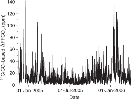
The hourly FFCO₂ offsets compared to background air at Jungfraujoch are displayed in Fig. 1, and are in the following referred to as ¹⁴C-calibrated CO-based ΔFFCO₂ or ¹⁴C/CO-based ΔFFCO₂. ¹⁴C/CO-based ΔFFCO₂ in Heidelberg frequently shows strong diurnal variation with amplitudes reaching more than 100 ppm during meteorological situations with exceptionally strongly suppressed atmospheric mixing during night and rigorous vertical mixing during day. We also frequently observe that, even during wintertime, the ΔFFCO₂ drops to values below 5 ppm. This feature is not found in previous studies using weekly integrated sampling of ¹⁴CO₂ (Levin et al., 2003; Levin and Rödenbeck, 2008). When using integrated sampling, the night-time enhancement in ΔFFCO₂ always overcompensates the few almost clean-air situations, which often occur in the afternoon. The ability to resolve these features is one of the key improvements when using the ¹⁴C/CO-based approach. The long-term mean of the ¹⁴C/CO-based ΔFFCO₂ is elevated by more than 10 ppm in Heidelberg compared to free tropospheric air (i.e. Jungfraujoch observations), which is consistent with studies based on integrated ¹⁴CO₂ alone (Levin et al., 2011). We also found that the ΔFFCO₂ concentration during winter is more than twice as high as in summer. This is expected to be a superposition of the altered vertical mixing (i.e. more vigorous in summer) and the seasonal variation of the FFCO₂ emissions. A seasonal emission change is predicted by the emission model (see Section 3.2 and also Fig. 3), and Vogel (2010) found a 75% increase of the night-time FFCO₂ fluxes during winter, using the radon-tracer method (e.g. Levin et al., 1999; Hammer and Levin, 2009; Vogel et al., 2012) in our domain. A similar seasonal variation of the FFCO₂ fluxes was also found by Levin et al. (2003).

Fig. 1 Hourly ¹⁴C-calibrated CO-based fossil fuel CO₂ offsets in Heidelberg relative to Jungfraujoch (cf. Section 2.1.).

2.2. ¹⁴C-based ΔFFCO₂ from grab samples

This study also uses the data of 189 whole-air grab samples collected during the years 2003–2009. This is an extension of the dataset described in Gamnitzer et al. (2006) and Vogel et al. (2010) of samples collected using a semi-automatic flask sampler (Neubert et al., 2004). The sampled air was analysed at the Heidelberg Combi-GC for trace gas concentration. Afterward, the remaining CO₂ was cryogenically extracted for ¹⁴CO₂ analysis. Most of the samples collected prior to 2005 were analysed by Accelerator Mass Spectrometry (AMS) at the Groningen Radiocarbon laboratory with a typical measurement uncertainty of ±5–10‰ (Gamnitzer et al., 2006). The samples collected from 2005 onwards were analysed at the AMS laboratory of the Max-Planck Institute for Biogeochemistry in Jena, Germany, with a typical measurement uncertainty of ±2–3‰. Using eq (1), this translates to an uncertainty in the ¹⁴C-based ΔFFCO₂ from these flasks of approximately 1 ppm for the more recent and approximately 2–3 ppm for the early samples.

2.3. Auxiliary observations of ²²²Rn and N₂O

To possibly attribute the model-observation deviations to specific components of the modelling framework, we also make use of the continuous observations of atmospheric ²²²Rn and N₂O concentration in Heidelberg. ²²²Rn is measured at the Heidelberg site at a separate intake ca. 20 m above ground. The ²²²Rn activity concentration is calculated from the measured activity of its daughter ²¹⁴Po that is attached to aerosols and collected on a static filter using the Heidelberg Radon-Monitor setup (Levin et al., 2002). The ²¹⁴Po decay on the filter is monitored with a commercial Canberra PIPS 900 AM detector from a solid angle of 0.265, assuming 100% efficiency of the detector. Our measurements are performed as half-hourly integrated atmospheric ²¹⁴Po activity concentrations on which we apply a disequilibrium correction of 1.367, which was determined experimentally by Cuntz (1997). All of the measured data are aggregated to hourly values. The N₂O observations used in Section 4.2 are part of the quasi-continuous in-situ measurements of the Heidelberg Combi-GC system (Hammer, 2008). The data are reported on the WMO2006 scale with a repeatability of ±0.15 ppb, determined from frequent target gas measurements.

3. Modelling framework

3.1. STILT modelling

In this study, we use the STILT model (Lin et al., 2003), which is based on the Hybrid Single Particle Lagrangian Transport model (HYSPLIT) (Model access via NOAA ARL Ready website: http://www.arl.noaa.gov/ready/hysplit4.html). The basic idea of the Lagrangian particle dispersion modelling approach is to determine the surface influence I( x _r ,t _r ∣x,t) on a receptor point x _r (or observation point in this study) at time t _r. This is achieved by simulating the trajectories for air parcels that arrive at the receptor. We can, therefore, calculate how much of the tracer has accumulated in each time step until it reaches the receptor (i.e. at t=t _r ). The initial concentration of the air parcel (at the boundary of our domain) is retrieved from a global simulation of atmospheric CO₂ (so-called analysed fields, available from http://www.bgc-jena.mpg.de/~christian.roedenbeck/download-CO₂–3D/) that uses TM3 in combination with fluxes optimised through an inversion (Rödenbeck et al., 2003).

To link surface fluxes F(x,t) and the discrete concentration change, compared to the initial concentration, (ΔC( x _r , t _r )), we utilise the so-called footprint f(x _r , t _r ∣x, t) (Gerbig et al., 2006).3

with m_air being the molar mass of air and ρ the air mass density below the mixed layer of height h*. Typically the footprint is given in units of [µmol/mol · m² s/µmol]. In this model, the surface fluxes F(x, t) (units: µmol per unit time) only affect the air parcel if it is close to the ground, i.e. at half the height of the well-mixed boundary layer h*. This is included in the definition of F(x,t), which is derived from a source and sink term S(x,t). A given flux in the units of [µmol m⁻² s⁻¹] at (x _i ,t _i ) during Δt can now be directly translated to a change in the mole fraction [µmol/mol] at (x _r ,t _r ). To calculate the footprints for our simulation, we used meteorological data of the European Center for Medium-Range Weather Forecast (ECMWF), with a 25 km×25 km spatial and a three-hourly temporal resolution. Hourly footprints were generated from 300 particles released at x _r with a back-trajectory time of 15 d to ensure the particles leave the local domain. Trajectories are computed with variable time-step size fulfilling the Courant–Friedrich–Lewy condition, for which not the resolution of the meteorological data was taken as the basis, but instead the desired higher resolution of the footprints with 10 km×10 km. The typical time-step for which the particle displacement is calculated is 15 minutes. Footprints are then computed with hourly time resolution, matching the maximum resolution of the fluxes. This framework is able to derive the expected concentration time series at the receptor with given flux maps and meteorological fields, from simplified physical properties. This parameterisation of transport still comprises some assumptions one has to be aware of. The linkage of surface fluxes to overlying air masses is parameterised in a simple way by one mixing height h*, and including all of the emissions if the particle is below 0.5 h*.

3.2. High-resolution emission model

The emission model used in this study was developed for the European domain by the Institute for Energy Economics and the Rational Use of Energy, University Stuttgart (IER) and will in the following be referred to as IER2005. It is based on disaggregating the national total emissions for CO₂, CH₄, N₂O and CO for the year 2005 taken from the official reports of the European countries to the United Nations Framework Convention on Climatic Change (UNFCCC).

3.2.1. Sectoral disaggregation of IER2005.

The national total emissions are reported in a sectoral structure based on the CRF (Common Reporting Format). The IER2005 emission model is split into 10 sectors according to the SNAP (Selected Nomenclature of Air Pollutants) definition of the EMEP/CORINAIR (European Monitoring and Evaluation Programme/CORe INventory of AIR emissions) atmospheric emission inventory guidebook (http://www.eea.europa.eu/publications/EMEPCORINAIR5). The IER2005 emission model uses these different SNAP sectors (i.e. SNAP1 to SNAP10) to allocate the sectoral emissions to sector-specific spatial proxies and temporal functions. The general methodology of the sectoral disaggregation is already described for previous versions of the IER2005 model (cf. Spatial and temporal disaggregation of anthropogenic greenhouse gas emissions in Europe: Emission Inventory for Europe 2005. Institut für Energiewirtschaft und Rationelle Energieanwendung. http://carboeurope.ier.uni-stuttgart.de/). The spatial and temporal disaggregation is done using available proxy data (cf. Table 1). A detailed description of the influence of the improvements in the methodology is given in Tiruchittampalam 2013 (‘Methoden und Modelle der räumlichen und zeitlichen Auflösung von Emissionen in Europa.’: manuscript in preparation). The sectoral emissions are treated as separate tracers in the transport model. This enables us to quantify the influence of a specific emission sector to the modelled ΔFFCO₂ concentrations later on. The dominant SNAP sectors in the IER2005 model for the Heidelberg catchment are combustion activities for heat and power generation (SNAP1, i.e. fossil fuel power plants), small combustion sources (SNAP2, i.e. combustion in manufacturing and non-industrial combustion, such as domestic heating), production processes (SNAP3/SNAP4, e.g. cement industry) and road traffic (SNAP7). This is in agreement with the emission patterns in the officially reported emissions from LUBW, the environmental agency of Baden-Württemberg (http://www.lubw.baden-wuerttemberg.de) for the relevant counties in the Heidelberg catchment area (i.e. Mannheim, Heidelberg, Rhine-Neckar).

Table 1. Distribution parameters in the IER2005 emission model

		Distribution parameter
SNAP	Short description	Spatial	Temporal
1	Energy production	Location of power plants, land use	Fuel use, load curves
2	Non-industrial combustion	Population density, land use	Fuel use, temperature dependent, load curves
3	Combustion in manufacturing	Facility location, employee numbers, land use	Production, holidays, shift times, temperature dependent load curves
4	Production processes	Facility location, employee numbers, land use	Production, holidays, shift times
5	Extraction and distribution of fossil fuel	Distribution network, facility location, land use	Constant
6	Solvent use	Employee numbers, population density, land use	Production, holidays, shift times
7	Road traffic	Road network, traffic counts, population density, land use	Traffic counts
8	Other mobile and machinery	Traffic volume, rail network, airport location, LTO-cycles, river network, population density, land use	Traffic counts, flight plans, passenger and freight numbers
9	Waste treatment and disposal	Waste statistics (e.g. municipality), facility locations, land use	Constant
10	Agriculture	Livestock statistics, crop statistics, land use	Animal activity, temperature

The minor emissions from SNAP5 (extraction and distribution of fossil fuels), SNAP6 (solvent use), SNAP8 (other mobile sources and machinery) and SNAP10 (agriculture) can be neglected. For N₂O though, the emissions from agriculture and waste treatment (SNAP9) account for a significant share of the anthropogenic emissions in the sites vicinity. The CO and CH₄ emissions are similarly split into the 10 source categories but are not further discussed in this study. Thus, in total we yield results for 40 different anthropogenic sector-pollutant combinations (4 compounds×10 sector categories) from the IER2005 model.

3.2.2. Spatial disaggregation of IER2005.

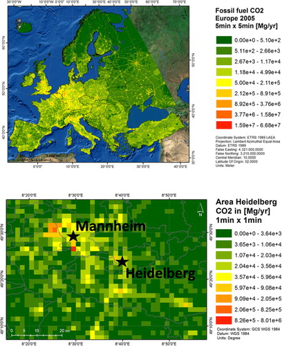
To produce a gridded high-resolution emission product, the spatial distribution is achieved by splitting the sources into three emission groups: (1) point sources, (2) line sources and (3) area sources. Point sources are, for example, power plants or large industrial sites. For power plants, the location of the emissions is well known, and one only has to disaggregate the overall emission of the energy sector based on independent information, for example, thermal power statistics and fuel use of individual power plants. For industrial facilities employee numbers are used in addition (cf. Table 1). Line sources such as roads, train tracks or waterways are spatially distributed using network maps, traffic counts as well as population density. Finally, area sources from rather diffuse emitting groups such as non-industrial combustion sources or emissions from animal husbandry in rural areas are the last type of emitters. As in other emission models, the spatial allocation of these emissions has the largest uncertainty (e.g. Pacala et al., 2010; Oda and Maksyutov, 2011; Nassar et al., 2013). The emissions can only be distributed using statistical data (e.g. livestock numbers for certain agricultural emissions). Another example is the spatial distribution of the emissions from domestic heating, which is done using population density and land use data. The set of parameters used to spatially distribute the emissions to all 10 SNAPs is given in Table 1. The spatial distribution of total annual mean anthropogenic CO₂ emissions for all sectors combined in Europe for 2005 on a 5 min×5 min grid is shown in Fig. 2 (upper panel). National boundaries are well distinguishable on this map, which is due to the methodology used to create this map based on disaggregation of total national emissions. For Germany, IER provided a data product with an even higher spatial resolution of 1 min×1 min. Figure 2 (lower panel) shows a zoom of this in the vicinity of our measurement site.

Fig. 2 Top: Map of the spatial distribution of FFCO₂ fluxes in the year 2005. Bottom: Annual mean emission of CO₂ in the immediate vicinity of the Heidelberg measurement site. The highly populated Heidelberg-Mannheim region is clearly visible as well as the large industrial area of Mannheim-Ludwigshafen. The coal-fired power plant in Mannheim approximately 20 km to the north-west of Heidelberg is also clearly distinguishable as the strongest single emitter in the region.

3.2.3. Temporal disaggregation of IER2005.

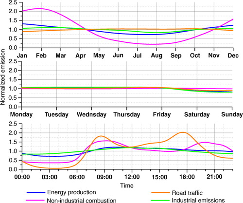
To derive emissions with hourly time resolution from annual values, one has to introduce time profiles that are related to the mean anthropogenic activities. Traffic and non-industrial combustion are particularly strongly coupled to domestic heating requirements and mobility, which is generally based on a deep-rooted regularity (Song et al., 2010). For the IER2005 emission model, the temporal disaggregation is done on monthly, weekly and diurnal time scales. These time curves are, of course, normalised to 1 to preserve the annual total emissions. (cf. Spatial and temporal disaggregation of anthropogenic greenhouse gas emissions in Europe: Emission Inventory for Europe 2005. Institut für Energiewirtschaft und Rationelle Energieanwendung. http://carboeurope.ier.uni-stuttgart.de/). The distribution parameters are given in Table 1. From the monthly time-curve of SNAP2 (non-industrial combustion), given in the upper panel of Fig. 3, we can see that its seasonal emission factor is highly variable. The seasonal variation is derived from a correlation of emission with temperature, which is parameterised with degree heating days. The seasonality of SNAP1 (energy production) is caused by the increased energy demand for heating and light during the winter. Industrial emissions are slightly reduced in the summer due to long summer holidays, while the road traffic is rather constant on that time-scale. The variations on a weekly time-scale are comparably small, and we only notice a slight decrease of emissions on the weekend, which fits with a common 5-d work week (Monday–Friday). On the sub-seasonal scale, the diurnal variation is the dominant signal. For road traffic (SNAP7), the diurnal variation is determined from hourly traffic counts. We see two distinct peaks during the morning and evening rush hour and hardly any emissions during the night-time. The non-industrial combustion emissions are distributed according to a more complex set of parameters, but basically mirror the fact that the emissions increase before people leave (to work) and the increased emissions in the evening after returning home. The emissions for energy production and industrial emissions do not show pronounced diurnal variations. The FFCO₂ emissions for a specific time are derived by multiplying by the according monthly, weekly and hourly factors. As different regions of Europe are subject to different climatic conditions, vacation schedules and other customs, IER2005 uses country-specific temporal profiles.

Fig. 3 Example of the temporal disaggregation of FFCO₂ emissions within the IER2005 emission model for energy production (blue), non-industrial combustion (magenta), road traffic emissions (orange) and industrial emissions (green). Emission factors for monthly (upper panel), day-to-day (middle panel) and hourly (lower panel) variations of FFCO₂ fluxes are shown.

3.2.4. Emission inventory for ²²²Rn.

To assess the model's ability to properly represent atmospheric mixing, especially in the vertical, we use the information from a tracer that is independent and complementary to FFCO₂. Here ²²²Rn is the best choice as it is purely natural (soil-borne) and has a rather homogeneous spatio-temporal flux pattern, if compared to the highly variable emissions of FFCO₂. In our modelling framework, we used the radon emission data of Szegvary et al. (2007) for Europe. The data have provided as weekly radon fluxes on a 0.5°×0.5° gridded map for 2006, and fluxes have been shown to predict fluxes reasonably well (Zhang et al., 2011). The annual mean flux from Szegvary et al. (2007) is also in line with the fluxes for our Heidelberg catchment area determined from regular long-term measurements (Schüßler, 1996), but lacks the seasonal variation of 25%.

4. Results and discussion

Before we try to utilise the combination of regional modelling, high-resolution emission model and observational data for any further interpretation, we evaluate how well our modelling framework is able to simulate the observational data. Using the sector-specific emission dataset, we can determine how much each sector is contributing to the total FFCO₂ offset. Using a STILT-ECMWF simulation, we found that the three largest annual contributors are energy production (28%), industrial emissions (26.5%) and non-industrial combustion (19.5%). The residual quarter originates from road traffic (15%) and six other sectors together contributing only 11% of the total.

We choose two sample episodes in February 2005, shown in Fig. 4, to illustrate situations where typical deviations between model simulations and observations are noticeable, that are also found throughout the full year of model simulation. Figure 4a shows the simulated ΔFFCO₂compared to the ¹⁴C-based ΔFFCO₂ from the grab samples and the ¹⁴C/CO-based ΔFFCO₂ estimate, including its one sigma uncertainty range. Generally, the model captures moderate concentration increases as seen from 7 February to 10 February and the slight increase of the lower envelope of ΔFFCO₂ beginning on 19 February.

Fig. 4 Two example episodes in 2005 of observational data and modelling results derived using STILT-ECMWF and the IER 2005 emission model. (A) ¹⁴C/CO-based ΔFFCO₂ measurements, including the 1-sigma uncertainty range (red band), solely ¹⁴C-based ΔFFCO₂ estimate from grab samples (blue dots), and the original modelling results (grey, dotted) as well as the ²²²Rn-corrected model (black line). (B) Sectors contributing to the total ΔFFCO₂ in the model, namely energy production (blue), non-industrial combustion (magenta), industrial emissions (green) and others in orange. (C) Modelled excess of N₂O in Heidelberg (black) and the local offset of N₂O derived from the observation. (D) Sectors contributing to the overall ΔN₂O in the model, energy production (blue), non-industrial combustion (magenta), industrial emissions (green) and others (orange), the latter including the strongly contributing sectors for N₂O: waste and agriculture.

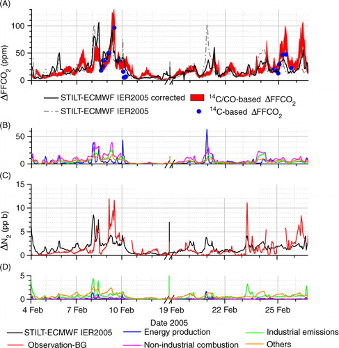
However, looking at individual events, we often find significant differences between the modelling results and the observations in both, phasing and amplitude. Here, the high values of 9 February seem somewhat underestimated, and for 26 February they are also not captured properly in the model simulations. To back our ¹⁴C/CO-based ΔFFCO₂ observations, we can use our grab sample data as a confirmation. The grab sample estimates are solely based on ¹⁴CO₂ measurements. We see that most of the ¹⁴C/CO-based data agree with the grab sample points within its one sigma uncertainty, with only three outliers on 10 February.

Throughout our dataset, we generally find two types of deviations: Firstly, an overestimation of night-time enhancements, which is a known problem when using the STILT model, as it tends to aggregate too much tracer during night-time because of an underestimation of the nocturnal boundary layer height (Denning et al., 1996; Gerbig et al., 2008; Kretschmer et al., 2012); this will be addressed later. Secondly, we occasionally detect strong short-term overestimations in the model simulation compared to the measured ¹⁴C/CO-based ΔFFCO₂. When analysing the contribution of the different emission sectors to the signal, shown in Fig. 4b, we find that these deviations are often due to a strong influence of SNAP1 (energy production) on our model results, seen here on 8 and 21 February. This seems to point to an overestimation of the fluxes in the emission model, which is a rather surprising finding, as the emissions from power plants are often assumed to be one of the best known (Olivier et al., 2005; Gurney et al., 2009). The CO₂ emissions from power plants are highly correlated with the thermal power statistics for the facility, which is used as a proxy in the IER2005 model. Investigation of the time series of an additional tracer, N₂O, leads us to doubt this simple solution. The regional enhancement of the observed N₂O is determined by subtracting the low-frequency component of the observations (lower envelope) and compared to the modelled N₂O offset (cf. Fig. 4c). Although, this approach is too simple to allow a quantitative assessment of N₂O fluxes it is apparent that for N₂O the main driver of the model-observation difference are industrial emissions (green line in Fig. 4d). In our case, they originate from adipic acid production and associated emissions in a nearby plant of the BASF Company in Ludwigshafen am Rhein, about 30 km Northwest of Heidelberg (see Schmidt et al., 2001). The emissions from the coal power plant and the chemical plant are not correlated, but they share one specific physical feature: both sources emit their effluent from high stacks in the same wind sector relative to Heidelberg. The fluxes of the emission inventories are (currently) only included in a simple way, i.e. including all or none of the emissions. This might not be sufficient when modelling the emissions from power plants and other large point sources that emit from stacks. As their effluent is often hot, it will be vertically distributed over an extended column, depending on the meteorological conditions (Pregger and Friedrich, 2009).

To accurately include power plant emissions, a future modelling study will have to address this problem of the vertical distribution of large emissions in detail. In cases where the used modelling framework cannot be modified accordingly, the simulated data from situations where the contribution of these source sectors are high should not be used for an assessment of model-observation differences. The additional information gained from using our insights about the N₂O observations, we implemented a selection that neglects data if we find an anomalously large N₂O enhancement (threefold) or a threshold of 40% contribution from SNAP1 to ΔFFCO₂ is surpassed. Setting this threshold is of course a trade-off between flagging erroneous simulation results without altering the dataset fundamentally. Analysing the histogram of the observation model differences, we found that the distribution is skewed due to those outliers. Choosing a cut-off of 40% contribution for SNAP1 corrects for this, while not significantly biasing the results of our ¹⁴C/CO-based ΔFFCO₂ time-series (overall mean, variability or mean diurnal cycle). With the chosen criteria, less than 11% of the overall data are neglected data.

4.1. Variability correction using ²²²Rn

To address the problem of the mentioned shortcomings of vertical mixing during night-time in our model, we exploit the additional information provided by using a model-data comparison for the transport tracer ²²²Rn. The idea of a ²²²Rn-based correction to assess the variability of a model has been previously applied by Gamnitzer et al. (2006) in a different setting. As the spatio-temporal variations of the ²²²Rn flux are rather small in the area of investigation (Schüßler, 1996; Szegvary et al., 2007), diurnal variations of the ²²²Rn activity concentration are dominated by vertical mixing. Thus, an overestimation of the ²²²Rn activity concentration during night-time in the model is a good indicator for underestimated vertical mixing. Comparing the night-time enhancement of the modelled ²²²Rn data with the observed time-series, we can estimate an hourly correction factor k(t)=ΔRn _obs (t)/ΔRn _mod (t), that accounts for the underestimated night-time mixing height, and adjust the modelled ΔFFCO₂ using this factor accordingly:4

We also find situations where the model underestimates ΔRn. These situations mostly appear in the afternoon. If the modelled and observed ²²²Rn offset agree within 1-sigma of their uncertainties, no correction is applied. Implementing the ²²²Rn correction improves the modelling results such that they overlap with the observations (cf. Fig. 4a). In the second part of the period, in particular, we see that the variability is now captured more realistically. For our two episodes of February 2005, the correlation coefficient R between the hourly ¹⁴C/CO-based ΔFFCO₂ and the STILT-ECMWF IER2005 time-series increases from 0.4 to 0.7 and the slope of the linear regression increases from 0.54±0.05 to 0.70±0.03, being still significantly smaller than one. The normalised standard deviation of the modelled time-series decreases from 1.27 to 1.03. The root mean square (RMS) error for our episodes is reduced from 7.3 ppm to 6.7 ppm. The large RMS error should be compared to the average ¹⁴C/CO-based ΔFFCO₂ estimate for this period of 21.2 ppm with a standard deviation of 17.4 ppm. We furthermore found an improvement when comparing the corrected simulated ΔFFCO₂ with the ¹⁴C-based flask samples where R improves from 0.3 to 0.7. The correlation between the ¹⁴C/CO-based approach and the ¹⁴C-based estimate is nevertheless still slightly higher (0.84). During extreme climatic conditions (e.g. prolonged droughts, extensive snow cover), we have, however, to be aware that this correction could have an adverse effect if the true ²²²Rn flux differs from the used ²²²Rn emission map. Especially as the currently available maps lack the seasonality, it is, thus, advisable to use/perform co-located ²²²Rn flux measurements wherever possible.

4.2. Comparison of mean diurnal cycles in summer and winter/early spring

In order to further assess the model-observation differences and investigate the effect of the radon correction, we now go from an episode-based discussion to an aggregated, yet still physically meaningful dataset. As we know from Section 3.2, the major component of the temporal structure of the emissions is the diurnal cycle. The variation of the boundary layer height also changes on diurnal time-scale. Therefore, we will be comparing mean diurnal cycles of the simulated and observed time-series. To account for the seasonal change in the mean fluxes as well as in the general mode of atmospheric mixing between summer (JJA) and winter (JFM), we choose to pool the data according to seasons (cf. Fig. 5). As shown in Vogel et al. (2010) with a slightly smaller data set, the ¹⁴C/CO-based approach compares well with the purely ¹⁴C-based data from our 189 grab samples pooled according to season and time of day. For the wintertime, our observational datasets show a significant peak in the morning hours and rather steady ΔFFCO₂ concentrations afterwards. For summer-time, we find that the ¹⁴C/CO-based approach tends to estimate a higher enhancement in ΔFFCO₂ during the morning and also a pronounced peak in the afternoon, which is not visible in the purely ¹⁴C-based dataset. This second peak found in the ¹⁴C/CO-based FFCO₂ in the late afternoon already described by Vogel et al. (2010) is not primarily caused by enhanced emissions, but likely an artefact of photo-chemically produced CO (Spivakovsky et al., 2000). The reduced height of the morning rush hour peak in the flask data could also partly stem from the fact that the data from 4 am to 9 am UTC have been pooled to one bin to achieve a robust result, thus smoothing the short strong enhancements found around 7 am UTC.

Fig. 5 Mean diurnal cycle of ΔFFCO₂ in Heidelberg pooled for A: winter (JFM) and B: summer (JJA). The ¹⁴C/CO-based regional ΔFFCO₂ is given in black with its 1-sigma uncertainty range in grey. The ¹⁴C-based ΔFFCO₂ from the grab samples is pooled according to the time of day and given in solid blue and the 1-sigma uncertainty range (dotted blue). The STILT-ECMWF results using the IER2005 emission model input are given in red, both the original data (dashed lines) and the ²²²Rn-corrected data (solid lines).

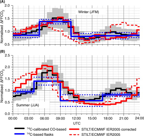
4.3. Mean diurnal cycle of the modelled ΔFFCO₂

With this basic understanding of the observational data, we can now investigate the difference between model and observations. The effect of the radon correction (from dashed red lines to solid red lines in Fig. 5) reduces the overestimation of the night-time accumulation of ΔFFCO₂ in the original model curve. We see that this variability correction leads to a real improvement of the overlap of model and observational data, for both summer and winter. Especially, the phasing of the morning hour peak is met more appropriately. For winter, the uncorrected model result shows a strong enhancement, which is driven by large FFCO₂ fluxes predicted by the emission model (cf. Fig. 3), which are emitted into a too-shallow boundary layer (as suggested by the mean diurnal cycle of radon, not shown). The radon-corrected mean diurnal cycle simulated by the model mostly lies within the 1-sigma uncertainty range of the ¹⁴C/CO-based observational data, still with slightly too high night-time concentrations, possibly indicating an overestimation of the underlying fluxes. For summer, we find that the modelling result does not display an afternoon peak and is more in line with the ¹⁴C-based FFCO₂ estimates of the grab samples. For the late afternoon, the uncertainty in the CO-based approach is too large (cf. Vogel et al., 2010), and the ¹⁴C-based ΔFFCO₂ estimate should be used as a reference. For the night-time, where ¹⁴C/CO-based ΔFFCO₂ is reliable, we find a significant deviation between model and observation. While the observational data do not show a marked increase between 0 and 4 o'clock UTC, the model overestimates ΔFFCO₂. Given that the ²²²Rn correction works for other times of the day, it seems more reasonable to assume that this deviation is caused by the temporal disaggregation of the emission model that might overestimate the emissions of some of the sectors during night time. Only interpreting the model-observation difference cannot unambiguously solve this problem as the other sectors could also be contributing to this increase. Looking at information about the emission inventory, we suspect that the sector, which is overestimated in its night-time pattern, is probably the industrial sector. This sector works on base of different production time schemes (one shift or multiple shift production). We would expect the decrease in heavy industry in Germany to influence the temporal patterns of SNAP3 and SNAP4 here. Therefore, we suggest that a stronger diurnal cycle (cf. Fig. 3 lower panel) than used in IER2005 might be appropriate. Although some problems cannot be solved satisfactorily, we can nevertheless identify the parts of the diurnal cycle that we can robustly estimate using modelling data and the parts where we have remaining uncertainties.

4.4. Separating diurnal cycle signals into source categories

To understand the driving sectors in the emission model, it is useful to split the FFCO₂ modelling result into its different emission groups, i.e. SNAP contributions. The model-observation comparisons might furthermore help improving the temporal disaggregation of the emission model or find leads towards processes in the modelling that have to be improved. Our observational ¹⁴C/CO-based ΔFFCO₂ data reveal that the general level and shape of the mean diurnal cycle changes throughout the year. With the help of the model data, we now want to gain insight in the driving process and on needs for future improvements in the emission model.

For January and February 2005 (Fig. 6a), the agreement between model simulation and ¹⁴C/CO-based estimates is particularly good. The rate of concentration increase during the night is met, as well as the rush hour peak. This indicates that both phasing and amplitude of the diurnal emission factors, which span one order of magnitude (cf. Fig. 3) in the IER2005 model, are appropriate here. From our model, we also learn that the non-industrial combustion (mainly domestic heating) sector (SNAP2) is by far the largest contributor during the winter months.

Fig. 6 Mean diurnal cycle of the local FFCO₂ offset for different months in 2005, A: January and February, B: March, C: June and July. The ¹⁴C/CO-based ΔFFCO₂ estimates (black, with 1σ uncertainties in grey) are compared to the radon-corrected STILT-IER2005 result (red) and the individual contributions to the modelling results (other colours).

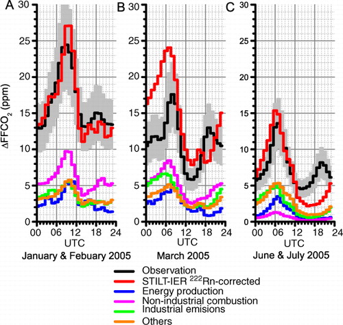
During the summer (Fig. 6c), the influence of the non-industrial combustion sector is significantly reduced. Given that the overall level is again nicely met can been seen as an indication that the tremendous seasonal emission factor change from winter to summer (210–29% of the annual mean) of SNAP2 in IER2005 is reasonable. From the model simulation, we learn that the contribution of the other main emission sectors is rather constant throughout the year. The largest contributors within these sectors are industrial emissions and road traffic (comprised in others). Hence, the slight overestimation of fluxes during the night (0–4 a.m. UTC, i.e. 2–6 a.m. local time) might be attributable to one of the two sectors. To understand the deviation post meridiem, seen in Fig. 6a, one has to bear in mind that, as in June and July, the afternoon peak of the observational data is likely enhanced by an artefact of using CO as proxy (Vogel et al., 2010); thus, it is impossible to quantify if the model-observation mismatch is significant. The fact that we do not find an afternoon peak in the modelled data can be traced back to a possibly adverse effect of the radon correction: During the late afternoon, the correction factor k(t) is smaller than 1 and diminishes this peak in the corrected model results.

The seasonally differing diurnal ΔFFCO₂ concentration variation is not only caused by changing diurnal variations of the emissions, but also due to changing area of influence, i.e. more influence from regions with larger or smaller average FFCO₂ fluxes. This is especially pronounced during March 2005, when the meteorological conditions often favoured air flow from the northeast. The ¹⁴C/CO-based ΔFFCO₂ observation for March 2005 (cf. Fig. 6b) lies in between the mean diurnal cycles of January and February, and June and July. Although the overall agreement of model simulation and data is good throughout our data set, there are specific situations and even whole months where significant deviations are found. Regarding the general level of ΔFFCO₂, March 2005 displays the largest deviation between model and observations for our entire record. March 2005 was considerably warmer than January and February 2005 [German weather service (DWD), station 05906, available historic data via web-interface. http://www.dwd.de]. However, we still find that the non-industrial combustion (domestic heating) sector is the largest contributor. Nevertheless, it is not reasonable to attribute the overestimation to an error in the used seasonal emission factors for SNAP2, as re-adjusting them would worsen the agreement in both summer and winter. We find that the industrial emissions also contribute to the overestimation of the night-time ΔFFCO₂ levels. During March 2005, the influence of the highly populated and industrialised region of Mannheim-Ludwigshafen (see Fig. 2) explains the strong contribution from industrial sources. We suspect that the emissions especially from diffuse sources could be overestimated in the spatial disaggregation used, as we know they have the largest uncertainties. To answer the question if this is the driving process, we can use information from the emission modelling community. Hoornweg et al. (2011) found that assuming an average per capita emission for regions or even cities can lead to a significant bias of the CO₂ emission estimates. For large German cities, the average per capita emissions are known to significantly differ, for example, 9.7 tons of CO₂ equivalent per capita for Hamburg and 16 tons of CO₂ equivalent for Stuttgart (Kennedy et al., 2009). In particular, the emissions from domestic heating, which depend on standard of living and housing infrastructure as well as heating systems (single heating systems, district heating and Combined Heat and Power systems), can deviate by more than a factor of 4, even within the same city for industrialised countries (Hoornweg et al., 2011). For Mannheim, 1.1 tons of CO₂ emitted per capita from non-industrial combustion are reported by the environmental agency of Baden-Württemberg (http://www.lubw.baden-wuerttemberg.de), while the average of the province of Baden-Württemberg is 2.3 tons CO₂ per capita. Accounting for these reduced per capita emissions would significantly decrease the model-observation mismatch in March. The decreased carbon intensity of urban living is not yet included in the available state-of-the-art emission model and presumably causes a general overestimation of ΔFFCO₂ for monitoring sites that experience situations with strong influence from urbanised regions. A framework like ours might be used to further investigate and quantify this effect in future studies.

5. Summary and conclusions

Our regional study could show that using a sector-specific high-resolution emission model of regional FFCO₂ is beneficial for understanding the observational data at the Heidelberg measurement site, as well as gaining insights where future improvements in the different components of the modelling framework are needed. Our investigation suggests that large emissions from stacks in our domain might cause strong sporadic deviations between the modelled time-series and the observed continuous ΔFFCO₂. By looking at the parameterisation of the surface influence, i.e. including all the emissions from stacks in the lowest layer, it became apparent that linking the emission model to the Lagrangian model in a simple way does not suffice. The effect of this truncation should be quantified in future modelling studies. It is apparent that, when only investigating the effect of this simplification, a much simpler framework would have been sufficient. However, it was the joint interpretation of ¹⁴C/CO-based ΔFFCO₂ and N₂O data that first lead to our re-evaluation of the underlying linking mechanism. A second strategy used in this study was to utilise ²²²Rn data to account for known problems in correctly modelling the amplitude of the boundary layer height variation. This variability correction largely improved the agreement between observations and modelling results for the mean diurnal cycle of ΔFFCO₂. Nevertheless, a straight forward quantitative assessment of the hourly emission model is still not feasible when solely relying on interpreting the model-observation mismatch, as the uncertainty contributed from the atmospheric transport model was still too large. The analysis of the model-observation deviations, however, helped identifying potential processes that cause model and observations to deviate. The difference in the mean diurnal cycle of ΔFFCO₂ in March 2005 implied that the domestic heating emissions (SNAP2) might be overestimated. A comparison of the reported per capita emissions of the biggest city in the source region (Mannheim) with the average per capita emission, used to disaggregate the emission from SNAP2, uncovered that only 50% per capita CO₂ emissions from the non-industrial combustion should be assumed for this city compared to the average of the province.

One could ask, if this difference between the parameterised emissions in the IER2005 model and the officially reported emissions by the environmental agency could have been found and corrected for without evoking a laborious model-observation comparison. The answer to this would have to be yes. We are convinced though that it is exactly this type of combined evaluation, involving observationists and modellers, that has the biggest chance of uncovering these differences. The model-observation mismatch can inform us about situations where the modelling framework is not able to reproduce the observed data correctly and forces us to address this issue. As all parties (i.e. emission modellers, atmospheric modellers and observationists) are involved, the difference is not simply attributed to one component, but we can utilise additional information, for example, other bottom-up emission data, to solve the problem.

The quantitative findings of this study are, of course, limited to the investigated domain. The approach of a joint assessment of a multi-tracer observation record and a sophisticated modelling framework, on the other hand, is applicable anywhere. Our finding that a simple per capita distribution of residential emissions is non-sufficient is applicable to any site in proximity to major urban centres. Other studies found similar results when investigating urban CH₄ emissions (Vogel et al., 2012). The possible influence of the simplified linking of emissions and transport should caution anyone working with observational datasets that are close to large facilities that emit from stacks. Finally, the variability correction using ²²²Rn is an approach that could be used for any model to investigate to which extends it suffers from the night-time rectifier effect. Both our approach or the previous one used by Gamnitzer et al. (2006) to correct erroneous vertical mixing in the REMO model (Karstens et al., 1996) can be helpful tools to generally assess the variability of the transport model in future greenhouse gas studies. To avoid any adverse effect of a radon correction, it is necessary to include the best possible ²²²Rn emission data. The currently available maps unfortunately still lack the seasonality suggested by plot-based studies for Europe (Schüßler, 1996; Jutzi, 2001). This type of investigation does not have to be restricted to ²²²Rn alone. For sites where ²²²Rn is not available, other tracers should be investigated for their usefulness to independently assess the diurnal variations of the boundary layer height. Ideally, one should, of course, try to include observations of the boundary layer height retrieved from radiosondes or LIDAR. These observations are unfortunately still rather sparse, but the information they provide is expected to advance the characterisation of rectifications and vertical mixing uncertainties in transport models (Kretschmer et al., 2012). Future observational networks for Greenhouse Gases, e.g. ICOS (http://www.icos-infrastructure.eu/), already foresee this type of auxiliary observations.

Besides identifying old and future challenges, i.e. coping with rectifier effects, implementation of emission from stacks, addressing simplifications in the emission model, this study also includes encouraging results. It was reassuring to find that both amplitude and general level of the mean diurnal cycle of ΔFFCO₂ change during the year in simulation and observations in a similar way. The mean level of ΔFFCO₂ of the radon-corrected model and the ¹⁴C/CO-based ΔFFCO₂ for summer and winter months were well compatible, which supports the strong seasonal and diurnal cycle in the emissions of FFCO₂ assumed in the emission model.

Although this study comprises different promising examples of how a comparison of regional-scale high-resolution modelling (both flux and transport) together with thoroughly calibrated ΔFFCO₂ observations can help to: (1) understand the observational data and (2) assess the modelling framework, this can only be seen as a first step. One that will hopefully spur more inter-disciplinary studies.

6. Acknowledgements

The authors gratefully acknowledge the careful processing of the ¹⁴C samples at the Heidelberg Radiocarbon laboratory of the Akademie der Wissenschaften at the Institut für Umweltphysik, the AMS laboratory at the Max-Planck Institut für Biogeochemie, Jena as well as Michael Sabasch and Renate Heinz for their diligent care of the trace gas measurements in Heidelberg. We thank one anonymous reviewer and Tomohiro Oda for their thoughtful and thorough reviews, which helped to significantly improve our manuscript. This work has been supported by the European Commission under the CarboEurope-IP (GOCE-CT2003-505572) and the ICOS Preparatory Phase Project (INFRA-2007-211574).

References

- Cuntz M . Der Heidelberger 222Radon-Monitor: Kalibrierung, Optimierung. 1997; University of Heidelberg, Heidelberg, Germany: Anwendung. Diploma Thesis.
- Cuntz M . Carbon cycle: a dent in carbon's gold standard. Nature. 2011; 477: 547–548.
- Denning A. S. , Collatz G. J. , Zhang C. , Randall D. A. , Berry J. A. , co-authors. Simulations of terrestrial carbon metabolism and atmospheric CO2 in a general circulation model: 1. Surface carbon fluxes. Tellus. B. 1996; 48: 521–542.
- Gamnitzer U. , Karstens U. , Kromer B. , Neubert R. E. M. , Meijer H. A. J. , co-authors . Carbon monoxide: a quantitative tracer for fossil fuel CO2?. J. Geophys. Res. 2006; 111: 22302.
- Geels C. , Gloor M. , Ciais P. , Bousquet P. , Peylin P. , co-authors . Comparing atmospheric transport models for future regional inversions over Europe. Part 1: mapping the CO2 atmospheric signals. Atmos. Chem. Phys. 2007; 7: 3461–3479.
- Gerbig C. , Körner S. , Lin J. C . Vertical mixing in atmospheric tracer transport models: error characterization and propagation. Atmos. Chem. Phys. 2008; 8: 591–602.
- Gerbig C. , Lin J. C. , Munger J. W. , Wofsy S. C . What can tracer observations in the continental boundary layer tell us about surface-atmosphere fluxes?. Atmos. Chem. Phys. 2006; 6: 539–554.
- Gerbig C. , Lin J. C. , Wofsy S. C. , Daube B. C. , Andrews A. E. , co-authors . Toward constraining regional-scale fluxes of CO2 with atmospheric observations over a continent: 1. Observed spatial variability from airborne platforms. J. Geophys. Res. Atmos. 2003; 108: 4756.
- Gurney K. R. , Law R. M. , Denning A. S. , Rayner P. J. , Baker D. , co-authors. Towards robust regional estimates of CO2 sources and sinks using atmospheric transport models. Nature. 2002; 415: 626–630.
- Gurney K. R. , Mendoza D. L. , Zhou Y. , Fischer M. L. , Miller C. C. , co-authors . High resolution fossil fuel combustion CO2 emission fluxes for the United States. Environ. Sci. Technol. 2009; 43(14): 5535–5541.
- Hammer S . Quantification of the regional H2 sources and sinks inferred from atmospheric trace gas variability. 2008; University of Heidelberg: PhD thesis.
- Hammer S. , Glatzel-Mattheier H. , Müller L. , Sabasch M. , Schmidt M. , Schmitt S. , co-authors . 2008. A gas chromatographic system for high-precision quasi-continuous atmospheric measurements of CO2, CH4, N2O, SF6, CO and H2, available at http://www.iup.uni-heidelberg.de/institut/forschung/groups/kk/GC_Hammer_25_SEP_2008.pdf .
- Hammer S. , Levin I . Seasonal variation of the molecular hydrogen uptake by soils inferred from continuous atmospheric observations in Heidelberg, southwest Germany. Tellus. B. 2009; 61(3): 556–565.
- Heimann M. , Keeling C. D . A three-dimensional model of atmospheric CO2 transport based on observed winds: 2. Model description and simulated tracer experiments. Aspects of Climate Variability in the Pacific and Western Americas. 1989; DC: Washington. Geophysical Monograph (ed. D. H. Peterson), Vol. 55, Max-Planck-Institut für Meteorologie, pp. 237–275..
- Hoornweg D. , Sugar L. , Gomez C. L. T . Cities and greenhouse gas emissions: moving forward. Environ. Urban. 2011; 23: 207–227.
- IPCC. Solomon S , Qin D , Manning M , Chen Z , Marquis M , etal. Climate change 2007: the physical science basis. Contribution of Working Group I to the Fourth Assessment Report of the Intergovernmental Panel on Climate Change. 2007; Cambridge: Cambridge University Press. pp. 135–145.
- Jutzi S . Verteilung der Boden-222Radon-Exhalation in Europa. 2001; Institut für Umweltphysik, Ruprecht-Karls Universität Heidelberg: State Examination Thesis.
- Karstens U. , Nolte-Holube R. , Rockel B . Calculation of the water budget over the Baltic Sea catchment area using the regional forecast model REMO for June 1993. Tellus. A. 1996; 48: 684–692.
- Kennedy C. , Ramaswami A. , Carney S. , Dhakal S . Greenhouse gas emission baselines for global cities and metropolitan regions. Proceedings of the 5th Urban Research Symposium. 2009. Marseille, France, 28–30 June 2009.
- Kretschmer R. , Gerbig C. , Karstens U. , Koch F.-T . Error characterization of CO2 vertical mixing in the atmospheric transport model WRF-VPRM. Atmos. Chem. Phys. 2012; 12: 2441–2458.
- Kromer B. , Münnich K. O . Taylor R. E. , Long A. , Kra R. S . CO2 gas proportional counting in radiocarbon dating—review and perspective. Radiocarbon After Four Decades. 1992; Springer-Verlag, New York. 184–197.
- Law R. M . Variations in modelled atmospheric transport of carbon dioxide and the consequences for CO2 inversions. Global. Biogeochem. Cycles. 1996; 10(4): 783–796.
- Levin I. , Born M. , Cuntz M. , Langendörfer U. , Mantsch S. , co-authors. Observations of atmospheric variability and soil exhalation rate of radon-222 at a Russian forest site. Technical approach and deployment for boundary layer studies. Tellus. B. 2002; 54: 462–475.
- Levin I. , Glatzel-Mattheier H. , Marik T. , Cuntz M. , Schmidt M. , Worthy D. E. J . Verification of German methane emission inventories and their recent changes based on atmospheric observations. J. Geophys. Res. 1999; 104: 3447–3456.
- Levin I. , Hammer S. , Eichelmann E. , Vogel F. R . Verification of greenhouse gas emission reductions: the prospect of atmospheric monitoring in polluted areas. Philos. Transact. A. Math. Phys. Eng. Sci. 2011; 369(1943): 1906–1924.
- Levin I. , Karstens U . Dolman A. J. , Freibauer A. , Valentini R . Quantifying fossil fuel CO2 over Europe. Observing the Continental Scale Greenhouse Gas Balance of Europe. 2007a; Springer-Verlag, Heidelberg. 245–250.
- Levin I. , Karstens U . Inferring high-resolution fossil fuel CO2 records at continental sites from combined 14CO2 and CO observations. Tellus. B. 2007b; 59: 245–250.
- Levin I. , Kromer B. , Schmidt M. , Sartorius H . A novel approach for independent budgeting of fossil fuel CO2 over Europe by 14CO2 observations. Geophys. Res. Lett. 2003; 30 2194..
- Levin I. , Münnich K. O. , Weiss W . The effect of anthropogenic CO2 and 14C sources on the distribution of 14CO2 in the atmosphere. Radiocarbon. 1980; 22: 379–391.
- Levin I. , Rödenbeck C . Can the envisaged reductions of fossil fuel CO2 emissions be detected by atmospheric observations?. Naturwissenschaften. 2008; 95(3): 203–208.
- Lin J. C. , Gerbig C. , Wofsy S. C. , Andrews A. E. , Daube B. C. , co-authors . A near-field tool for simulating the upstream influence of atmospheric observations: the Stochastic Time-Inverted Lagrangian Transport (STILT) model. J. Geophys. Res. 2003; 108 4493..
- Nassar R. , Napier-Linton L. , Gurney K. R. , Andres R. J. , Oda T. , co-authors . Improving the temporal and spatial distribution of CO2 emissions from global fossil fuel emission data sets. J. Geophys. Res. 2013; 118: 917–933.
- Neubert R. E. M. , Spijkervet L. L. , Schut J. K. , Been H. A. , Meijer H. A. J . A computer-controlled continuous air drying and flask sampling system. J. Atmos. Ocean. Technol. 2004; 21: 651–659.
- Nisbet E. , Weiss R . Top-down versus bottom-up. Science. 2010; 328(5983): 1241–1243.
- Oda T. , Maksyutov S . A very high-resolution (1 km×1 km) global fossil fuel CO2 emission inventory derived using a point source database and satellite observations of night-time lights. Atmos. Chem. Phys. 2011; 11: 543–556.
- Olivier J. G. J. , Van Aardenne J. A. , Dentener F. J. , Pagliari V. , Ganzeveld L. N. , co-authors . Recent trends in global greenhouse gas emissions: regional trends 1970–2000 and spatial distribution of key sources in 2000. Environ. Sci. 2005; 2(2–3): 81–99.
- Pacala S. W. , Breidenich C. , Brewer P. G. , Fung I. Y. , Gunson M. R. , co-authors. Verifying Greenhouse Gas Emissions: Methods to Support International Climate Agreements. 2010; Committee on Methods for Estimating Greenhouse Gas Emissions; National Research Council, National Academic Press, Washington, D.C.
- Peters W. , Jacobson A. R. , Sweeney C. , Andrews A. E. , Conway T. , co-authors. An atmospheric perspective on North American carbon dioxide exchange: CarbonTracker. Proc. Natl. Acad. Sci. 2007; 104(48): 18925–18930.
- Peylin P. , Houweling S. , Krol M. C. , Karstens U. , Rödenbeck C. , co-authors . Importance of fossil fuel emission uncertainties over Europe for CO2 modelling: model intercomparison. Atmos. Chem. Phys. 2011; 11: 6607–6622.
- Pregger T. , Friedrich R . Effective pollutant emission heights for atmospheric transport modelling based on real-world information. Environ. Pollut. 2009; 157(2): 552–560.
- Rödenbeck C. , Houweling S. , Gloor M. , Heimann M . Time-dependent atmospheric CO2 inversions based on interannually varying tracer transport. Tellus. B. 2003; 55: 488–497.
- Schimel D. , Alves D. , Enting I. , Heimann M. , Joos F , Raynaud D. , co-authors . Houghton J. T , Meira Filho L. G , Callander B. A , Harris N , Kattenberg A , Maskell K . Radiative forcing of climate change. Climate Change 1995: The Science of Climate Change. 1996; New York: Cambridge University Press. 65–131. chap. 2.
- Schmidt M. , Glatzel-Mattheier H. , Sartorious H. , Worthy D. E. J. , Levin I . Western European N2O emissions: a top-down approach based on atmospheric observations. J. Geophys. Res. 2001; 106: 5507–5516.
- Schüßler W . Effektive Parameter zur Bestimmung des Gasaustauschs zwischen Boden und Atmosphäre. 1996; University of Heidelberg, Germany. PhD thesis.
- Song C. , Qu Z. , Blumm N. , Barabasi A . Limits of predictability in human mobility. Science. 2010; 327(5968): 1018–1021.
- Spivakovsky C. M. , Logan J. A. , Montzka S. A. , Balkanski Y. J. , Foreman-Fowler M. , co-authors. Three-dimensional climatological distribution of tropospheric OH: update and evaluation. J. Geophys. Res. 2000; 105: 8931–8980.
- Szegvary T. , Conen F. , Stöhlker U. , Dubois G. , Bossew P. , co-authors. Mapping terrestrial γ-dose rate in Europe based on routine monitoring data. Radiat. Meas. 2007; 42: 1561–1572.
- Turnbull J. C. , Miller J. B. , Lehman S. J. , Tans P. P. , Sparks R. J. , co-authors. Comparison of 14CO2, CO, and SF6 as tracers for recently added fossil fuel CO2 in the atmosphere and implications for biological CO2 exchange. Geophys. Res. Lett. 2006; 33: L01817.
- Vogel F. R . 14CO2-calibrated carbon monoxide as proxy to estimate the regional fossil fuel CO2 component at hourly resolution. 2010; Ruprecht-Karls University Heidelberg, Germany. PhD thesis.
- Vogel F. R. , Hammer S. , Steinhof A. , Kromer B. , Levin I . Implication of weekly and diurnal 14C calibration on hourly estimates of CO-based fossil fuel CO2 at a moderately polluted site in southwestern Germany. Tellus. B. 2010; 62: 512–520.
- Vogel F. R. , Ishizawa M. , Chan E. , Chan D. , Hammer S. , co-authors . Regional non-CO2 greenhouse gas fluxes inferred from atmospheric measurements in Ontario, Canada. J. Integr. Environ. Sci. 2012; 9: 41–55.
- Zhang K. , Feichter J. , Kazil J. , Wan H. , Zhuo W. , co-authors. Radon activity in the lower troposphere and its impact on ionization rate: a global estimate using different radon emissions. Atmos. Chem. Phys. 2011; 11(15): 7817–7838.