Analysis and evolution of air quality monitoring networks using combined statistical information indexes

Abstract

In this work, we present combined statistical indexes for evaluating air quality monitoring networks based on concepts derived from the information theory and Kullback–Liebler divergence. More precisely, we introduce: (1) the standard measure of complementary mutual information or ‘specificity’ index; (2) a new measure of information gain or ‘representativity’ index; (3) the information gaps associated with the evolution of a network and (4) the normalised information distance used in clustering analysis. All these information concepts are illustrated by applying them to 14 yr of data collected by the air quality monitoring network in Santiago de Chile (33.5 S, 70.5 W, 500 m a.s.l.). We find that downtown stations, located in a relatively flat area of the Santiago basin, generally show high ‘representativity’ and low ‘specificity’, whereas the contrary is found for a station located in a canyon to the east of the basin, consistently with known emission and circulation patterns of Santiago. We also show interesting applications of information gain to the analysis of the evolution of a network, where the choice of background information is also discussed, and of mutual information distance to the classifications of stations. Our analyses show that information as those presented here should of course be used in a complementary way when addressing the analysis of an air quality network for planning and evaluation purposes.

• information theory
• optimal network design
• air quality monitoring
• Santiago de Chile

1. Introduction

The objectives of a monitoring network are multiple and usually include: compliance of air quality standards, which in turn may trigger control procedures, evolution of air quality and efficiency of curbing measures, and impacts on human health, ecosystems and climate, and so on (see e.g. Ainslie et al., 2009). Also, optimal network design must take into consideration practical constrains related to costs, security, and so on. Thus, the question of how to best sample airborne pollutants in a monitoring network is non-trivial. Over the last two decades or so, an increasing amount of research has been oriented towards optimal network design, particularly in the area of air quality, for example, Caselton and Zidek (1984); Haas (1992); Pérez-Abreu and Rodríguez (1996); Zidek et al. (2000); Chow et al. (2002); Elkamel et al. (2008); Pesch et al. (2008); Ruiz-Cárdenas et al. (2010); Zidek and Zimmerman (2010); Saunier et al. (2011); Wu and Bocquet (2011); Ruiz-Cárdenas et al. (2012).

Among the multiple statistical approaches to evaluate and optimise monitoring networks, we apply here statistical indexes tied to Shannon's information theory (Shannon, 1948) and Kullback–Leibler divergence (Kullback, 1959), in particular, those derived from the concepts of information gain and mutual information. The novelty is that we use both concepts in a complementary manner and in a normalised version considering what we call information gain or ‘representativity’, and mutual information or ‘specificity’ indexes. The information gain index relates to the contribution of a station to the total information of a network (‘representativity’), while the mutual information index refers to the amount of information provided by a single station that cannot be retrieved from other stations in a network (‘specificity’). Using solely one of these indexes results in misleading conclusions and they must be applied in a complementary way. We will illustrate the use of these concepts by applying them to air quality data collected in Santiago de Chile (33.5 S, 70.5 W, 500 m a.s.l.) between 1997 and 2010, where air pollution is an issue of concern, and where air quality monitoring has taken place since the late 1980s, and regularly within the framework of an attainment plan since 1997 (e.g. Gallardo et al., 2012a). The current network configuration is shown in Fig. 1 and described in Table 1. This air quality network was primarily conceived to address the compliance of air quality standards intended to protect the population from adverse health impacts. Today, it is still largely devoted to evaluate the compliance or not of air quality standards, particularly those related to inhalable particulate matter. Its ability to do so has been partially evaluated on the basis of statistical tools. Silva and Quiroz (2003) applied mutual information to classify the stations in Santiago, suggesting downtown stations as those that could be expendable if authorities wanted to re-distribute those stations. Gramsch et al. (2006) used principal component analysis and clustering techniques to identify groups of stations with similar behaviour in terms of emission patterns. We revisit those analyses using more general indexes and currently available data in a larger set of air quality network stations.

Fig. 1 Location of monitoring stations in Santiago's air quality network since the 1980's (for details see text). The symbols correspond to the names of the stations A: Gotuzzo, B: Providencia (not used in this study, in white), F: Independencia, L: La Florida, M: Las Condes, N: Parque O'Higgins, O: Pudahuel, P: Cerrillos, Q: El Bosque (seven stations continuously working on the period 1997–2008, in grey), R: Cerro Navia, S: Puente Alto, T: Talagante, V: Quilicura (four more stations added on the period 2009–2010, in black). The limit of the current urban area is indicated by a heavy line. Main topographic features of the Santiago basin are also shown.

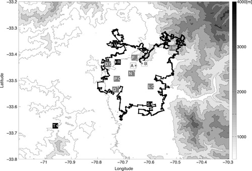
Table 1 Description of the air quality monitoring stations belonging over time to Santiago's monitoring network and the two periods of data used in this study.

	Period and data used			Lon	Lat	Height
		Char	Name	W	S	m a.s.l.	Type	Working
	Not used	A	Gotuzzo	70 655	33 444	576	Commerce/services	1988–1997
		B	Providencia	70 631	33 436	592	Close to main road/medium income	1988–2002
2009–2010 (PM10, PM2.5, O3)	1997–2008 (CO, PM10, O3, SO2)	F	Independencia	70 649	33 419	565	Commerce/services	Since 1988
		L	La Florida	70 586	33 513	594	Residential/low-medium income	Since 1997
		M	Las Condes	70 523	33 374	775	Residential/high income	Since 1988
		N	P. O'Higgins	70 658	33 461	545	In a park/close to highway	Since 1988
		O	Pudahuel	70 748	33 435	494	Residential/low income	Since 1997
		P	Cerrillos	70 713	33 493	511	Residential/industrial	Since 1997
		Q	El Bosque	70 664	33 544	582	Residential/industrial	Since 1997
		R	Cerro Navia	70 733	33 430	498	Residential/low income	Since 2008
		S	Puente Alto	70 593	33 591	680	Residential/low income	Since 2009
		T	Talagante	70 951	33 673	401	Rural	Since 2009
		V	Quilicura	70 747	33 365	489	Residential/low-medium income	Since 2009

The article is organised as follows. In Section 2, we review and define several statistical information indexes in a general setting. Section 3 describes the data sets considered in this study along with the main emission and circulation patterns of Santiago. Section 4 shows the application of ‘specificity’ and ‘representativity’ indexes. The evolution of the network between the late 1980s and the present in terms of information content is shown in Section 5. We perform clustering analysis using information distance in Section 6. Finally, summary and conclusions are presented in Section 7.

2. Statistical information indexes for network analysis

We present in this section some statistical information indexes for evaluating air quality monitoring networks based on the concept of relative information by Kullback and Liebler as described in Kullback (1959). More precisely, we introduce four indexes: (1) complementary relative mutual information or ‘specificity index’, (2) relative information or ‘representativity index’, (3) information gaps associated with the evolution of a network and (4) normalised information distance used in clustering analysis.

These indexes are all defined for arbitrary probability densities but we provide the formulas to compute them in the particular case of normally distributed densities. In fact, most of the information indexes presented here will be applied assuming that the underlying statistical densities of the measurements are log-normal so when we refer to the measurements in the normal case we implicitly mean the logarithm of the measurements. Notice that (see Table 2) other distributions could better fit the measurements, as is the case of gamma distributions, but no simple expressions for the Kullback–Liebler divergence for multivariable gamma densities are known, except for the bivariate case (see e.g. Chatelain et al., 2008) even if it seems theoretically plausible (see Nielsen and Nock, 2010). Therefore, we only consider the log-normal multivariate case in this study.

Table 2 Relative quadratic error in percentage using different statistical models for fitting the 1997–2008 data for 7 stations and 4 measured species and for the 2009–2010 data for 11 stations and 3 measured species.

	Normal			Log-normal			Gamma
	All	S	W	All	S	W	All	S	W
For fitting the 1997–2008 hourly data
CO	26.9	24.1	18.1	14.9	23.9	10.9	5.17	8.07	4.66
O3	9.76	10.5	8.99	11.1	19.7	8.87	3.93	10.5	2.06
PM10	10.5	6.46	8.96	1.87	1.50	3.94	0.63	0.41	1.17
SO2	37.1	42.7	26.0	41.1	40.2	30.5	21.0	24.2	12.7
For fitting the 2009–2010 hourly data
PM10	16.3	7.63	8.55	1.78	1.08	3.38	2.25	0.70	1.06
PM2.5	9.84	4.69	9.59	1.36	1.49	2.29	0.71	0.48	0.95
O3	10.9	12.6	6.79	9.81	16.9	6.89	3.85	9.78	3.30

All data (All), segregated by summer (S: Dec, Jan, Feb) or winter (W: Jun, Jul, Aug) months.

All the aforementioned indexes can be derived from the Kullback–Liebler divergence or relative information of a distribution q _X with respect to other reference distribution p _X :1

where X represents the multivariate random vector of measurements and the integral is taken over all the possible outcomes x. Then, if there are n stations and m species, the previous integral is in n×m variables and it is difficult to compute in practice. In the normal case, , with mean µ ₀, µ ₁ and invertible covariance matrices Σ₀, Σ₁, the expression for KL(p _X || q _X ) simplifies to2

where tr and |·| denote, respectively, the trace and determinant of the corresponding matrices and Ax ² where A is a matrix and x is a vector is a short notation for the inner product x ^T Ax. Notice that KL(p || q) is always non-negative (essentially since α–1–ln α≥0 for α>0), invariant against any invertible transformation, non-symmetric and it vanishes only if p _X =q _X .

In the following sections, we consider n monitoring stations with measurements of m different species given by the vectors X ₁,…, X _n and complementary measurement vectors , where represents the measurements of all the stations except for the i-th station. The total measurement vector of the whole network is then (rearranged in increasing index order) for any i=1,…, n.

2.1. Mutual information and specificity index

The mutual information between the station i and its complementary stations is given by

where , are the marginal densities for the measurements of station i and its complement, respectively and p _X is the joint density distribution of all the measurements. If all the densities are normally distributed, , , , with marginal covariance matrices , and joint covariance Σ _X then the mutual information can be simply computed from (2) as follows:

We define the specificity index s _i associated with the i-th station as the complementary relative mutual information given by (max _j stands for the maximum over j∈{1,…, n}):3

The specificity index measures how difficult it is to reproduce the measurements of the i-th station from the measurements of the other stations. We have 0≤s _i ≤1 and the station with highest specificity in the network corresponds to higher s _i (not necessarily 1) and the station with lowest specificity to the minimum s _i (always 0). The definition s _i is quite arbitrary since we could replace it by any other decreasing function of . For instance is another choice. We can also consider an index between 0 and 1 by defining (we use this choice to build Figs. 4, 5 and 7)

In any case, we are interested in the ordering induced by this index which is independent of the decreasing function of you may choose.

The definition we have chosen corresponds exactly to the concept of effectiveness already present in the literature (e.g. Pérez-Abreu and Rodríguez, 1996; Silva and Quiroz, 2003). Nevertheless, we consider that the denomination ‘effectiveness’ could lead to confusion. Indeed, the index s _i is a relative measure of information and it does not consider the total information of the network itself as it was already noticed in Bocquet (2009). Hence, a complementary index taking into account this intrinsic information of the network should be introduced to better evaluate if an station is effective or not. Following this remark, we introduce a new index in the next subsection.

2.2. Information gain and representativity index

If we represent by the densities and p _X the situations before and after the measurements X _i are known, then the information gain achieved by the measurements of the i-th station is defined by

Notice that, in order to model , we will need some a priori background information about the measurements at the i-th station. Let us precise this statement for the normal case. We take as in the previous section and, if and B _i are some a priori background mean and covariance that characterise the situation without knowledge at the i-th measurement site, we choose where , denote the mean and diagonal by block's covariance matrix with increasing ordering of indexes. With this, using that from (2) we obtain4

Notice that if and , then one can reproduce from the previous formula the expression for mutual information.

Notice that in our applications, the interesting case corresponds to

(reduction of uncertainty after the i-th-station is gauged) so we could also define the information gain as with a similar behaviour. Moreover, we could also select the simpler and classical definition (entropy decrease or Shannon information increase). Nevertheless, in practice, we found useful to include the term giving more representativity to measurements with high averages ( will be taken to be of zero mean value) and this naturally arises from Kullback–Liebler divergence. In this sense, the approach chosen in this study based on the definition of information gain from Kullback–Liebler divergence is near but not totally equivalent to the so-called entropy-based network design methods introduced by Zidek and collaborators (see Caselton and Zidek, 1984; Le and Zidek, 2006; Ainslie et al., 2009 and references therein).

We define the representativity index r _i of the i-th station as the relative information gain by5

The representativity index r _i represents the relative information gain after adding the i-th station to the network. This definition is also arbitrary and can be replaced by another increasing function of . For instance, in order to have an index between 0 and 1 (we use this choice to build Figs. 4, 5 and 7) we could take

In any case, we are interested in the ordering induced by this index which is independent of the increasing function of you may choose.

Concerning the background mean and covariance, in this work we will simply take

where µ _ij and σ _b,ij are a priori mean and standard deviations of the measurements of the j-th species in the i-th station.

Notice that other choices are possible. For instance, one could take into account the knowledge about the spatial distribution of the measuring sites by estimating the background values for the i-th measurement site as the optimal interpolation obtained from all other stations where geostatistical or other dispersion space embedding methods can be introduced (see Ainslie et al., 2009). This aspect is beyond the scope of this study, and for the sake of simplicity, we decided to introduce our indexes using diagonal covariace matrices. Nevertheless, in order to illustrate the importance of this point, we consider in the last sections a different choice of a priori covariances estimated from Barnes-type interpolation for a single species.

More generally, we can compute the information gain associated with a subset of stations K⊂{1,…,n} of cardinality k by

where the density represents the situation of the network with the complementary stations K ^c . In the normal case, where and , where y are obtained after eliminating all the components of µ _X and all the rows and columns of Σ _X associated with K, and , B _j are background mean and covariance matrices associated with each station in K as before.

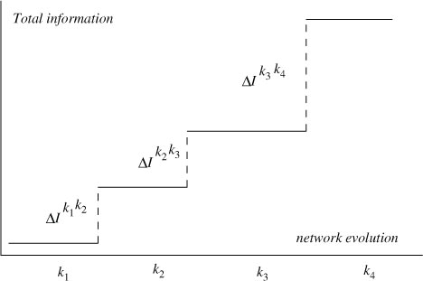
2.3. Evolution of total information and information gaps

Suppose we change the active monitoring stations in the network from K ₁ to K ₂, both subsets of {1,…,n} with cardinalities k ₁ and k ₂, and that we represent the situations before and after this change by the densities and . We define the information gap or change associated with this evolution by6

Notice that the information gap can be positive or negative and it is additive, that is, . In the particular case where K ₁⊆K ₂ and the measurements are normally distributed the information gain is exactly the (non-negative) quantity . This is true if the a priori information does not change after changing the configuration of the network, otherwise (6) is more general.

Using this concept, we can compute the successive gaps or changes in information content over the evolution of a network on the basis of the data corresponding to the final configuration of n stations (see Fig. 2). Thus, in order to compare past and present configurations of the network we can use current measurements.

Fig. 2 Schematic evolution of the total information of the network.

2.4. Normalised information distance and clustering

The mutual information between two stations i and j is given by7

The normalised information distance between two stations i and j is defined as in Coeurjolly et al. (2007):8

where is the Shannon entropy of the measurements X _i . This distance is zero only if and are independent and it is equal to one if i=j. Notice that in the normal case, for one species, we have

where ρ _ij is Pearson's correlation coefficient. Thus, the normalised information distance d _ij is strongly related to Pearson's distance . But, for non-normal distributions zero correlation does not imply independence and zero mutual information does. Therefore, since (7) and (8) are easy to compute without assuming any normality, it is always better to use the normalised information distance d _ij instead of Pearson's distance for measuring statistical independence, notably, when performing clustering analysis of the network stations, where the normal or log-normal fit of data is only approximate.

3. Santiago's characteristics

The city of Santiago is located in a semi-arid basin (annual rainfall less than 350 mm) in the central part of Chile bounded by the Andes Cordillera (4500 m altitude on average) to the East, a lower parallel mountain range to the West (1500 m altitude on average), and two east-to-west mountain chains to the North and South of the basin, respectively. The climate of Santiago is characterised by the quasi-permanent influence of the subtropical Pacific high, and the intrusion of occasional cold fronts, which bring precipitation in wintertime. The South Pacific high determines quasi-stagnant anti-cyclonic conditions that are further intensified, especially in fall and winter by the presence of sub-synoptic features known as coastal lows (e.g. Gallardo et al., 2002; Garreaud et al., 2002). There is a characteristic thermally driven circulation that defines up-slope south-westerly winds in the afternoon and down-slope north-easterly winds in the night and morning hours, more strongly so in summer (e.g. Saide et al., 2011).

The regional office of the Ministry of Health was in charge of monitoring Santiago's air quality from the late 1980s until 2011. Nowadays, this activity is continued by the recently created Ministry for the Environment. A historic record of the data (1988–2008) is available (as in September 2012) on the internet via the Chilean Ministry of Health at http://www.seremisaludrm.cl and http://www.asrm.cl. A copy of those data and of data collected in stations currently in operation can be found at the web page of the Chilean Ministry for the Environment at http://sinca.mma.gob.cl. Instruments and quality control procedures of the Santiago monitoring network follow recommendations from the Environmental Protection Agency of the United States of America, and are subject to public scrutiny and to occasional external review panels.

The specific air quality standards applied over time in Santiago can be found elsewhere in the literature (e.g. Zhu et al., 2012) that synthesises the situation in various megacities, including South American cities and Santiago.

The species measured are so-called criteria pollutants: carbon monoxide (CO), sulphur dioxide (SO₂), ozone (O₃) and partially inhalable particles (PM₁₀). Since 2000, nitrogen oxides are measured at three stations, and fully inhalable particles (PM_2.5) at four stations. In the current configuration all species are measured at all stations. Wind velocity, temperature, relative humidity are also continuously measured at the monitoring stations. The network's configuration is shown in Fig. 1. In sum, there are seven stations (F, L, M, N, O, P and Q) for which rather continuous and simultaneous time series are available for the period between 1997 and 2008 for carbon monoxide (CO), sulphur dioxide (SO₂), ozone (O₃) and partially inhalable particles (PM₁₀). We will restrict the analyses of ‘specificity’ and ‘representativity’ to this set of data. Evolution and clustering will consider PM₁₀, PM_2.5 and ozone data collected in the current network configuration, that is, for 11 stations (F, L, M, N, O, P, Q, R, S, T and V) operating in 2009 and 2010. We provide some basic descriptive statistics for each measured species at each station (see Table ^{Table 3} and 4 ^{Table 4}).

Table 3 Main statistics (mean, standard deviation and maximum) for each of the 7 monitoring stations working during the period 1997–2008 based on hourly averages during all the year (All), summer (S: Dec, Jan, Feb) and winter (W: Jun, Jul, Aug).

Species		F	L	M	N	O	P	Q
CO (ppb)	All	1.2	1.2	0.7	1.6	1.1	1.4	1.2
		1.1	1.2	0.5	1.7	1.4	1.4	1.3
		5.5	6	2.8	8.6	8.8	6.7	6.9
	S	0.5	0.6	0.4	0.6	0.4	0.5	0.6
		0.4	0.4	0.2	0.5	0.3	0.5	0.5
		4.4	5.1	1.9	5.7	4.1	4	6.7
	W	1.8	1.9	1.0	2.2	1.8	1.9	1.9
		1.2	1.4	0.6	1.9	1.8	1.6	1.6
		5.5	6	2.8	8.6	8.8	6.7	6.9
O3 (ppb)	All	19.6	21.2	24.9	23.1	19.0	20.1	20.3
		17.0	20.0	24.4	18.6	15.9	16.5	16.3
		71	82	106	78	64	69	66
	S	23.3	27.1	33.4	27.2	23.3	24.7	24.4
		18.4	21.7	27.9	19.3	16.6	17.0	17.2
		71	82	106	78	64	69	66
	W	12.4	12.5	13.7	14.9	11.8	12.6	12.9
		11.4	13.4	13.8	13.9	11.6	12.3	11.6
		71	82	106	78	64	69	66
PM10 (µg/m^3N)	All	72.1	80.9	56.7	74.2	77.8	75.9	80.3
		43.5	53.8	36.7	50.6	58.4	52.7	54.9
		244	309	197	288	359	293	312
	S	57.7	68.5	54.3	57.7	62.6	64.4	66.5
		28.2	34.0	29.1	30.8	36.8	38.2	33.7
		239	309	196	286	358	293	290
	W	88.3	94.4	57.9	92.6	95.9	90.9	94.7
		52.6	67.2	43.2	61.9	73.6	63.6	67.8
		244	309	197	288	359	293	312
SO2 (ppm)	All	4.97	4.46	3.43	5.02	4.1	4.96	5.05
		3.4	3.3	2.1	3.7	2.7	3.4	3.8
		22	23	14	23	16	21	27
	S	4.0	3.6	3.0	3.8	3.2	3.8	4.3
		2.6	2.8	1.9	2.8	2.0	2.5	3.6
		22	23	14	23	16	21	27
	W	6.3	5.2	3.9	6.4	5.1	6.5	5.9
		4.0	3.6	2.3	4.3	3.1	3.9	4.0
		22	23	14	23	16	21	27

Table 4 Main statistics (mean, standard deviation and maximum) for each of the 11 monitoring stations working during the period 2009–2010 based on hourly averages during all the year (All), summer (S: Dec, Jan, Feb) and winter (W: Jun, Jul, Aug).

Species		F	L	M	N	O	P	Q	R	S	T	V
O3	All	17.0	18.4	19.2	21.9	15.2	18.6	16.3	16.0	20.1	17.1	16.1
(ppb)		16.0	18.2	20.4	17.0	14.6	15.5	15.0	14.9	16.5	11.7	15.5
		66	73	88	69	59	64	60	60	65	51	63
	S	21.5	25.3	28.0	26.0	21.0	24.3	21.8	21.3	25.2	18.6	22.1
		17.8	20.5	24.1	18.0	16.0	16.6	16.9	15.9	17.6	11.7	16.7
		66	73	88	69	59	64	60	60	65	51	63
	W	8.6	9.4	8.8	13.0	8.2	10.7	9.0	8.2	12.3	12.6	8.0
		8.5	9.6	9.2	10.3	8.5	9.2	8.2	8.3	11.0	9.9	8.9
		62	68	67	67	54	63	60	58	64	50	61
PM10 (µg/m^3N)	All	50.1	57.1	45.7	55.8	48.3	58.9	61.9	52.3	49.5	37.4	73.3
		22.8	24.2	22.1	26.5	23.2	28.5	27.4	24.8	21.4	20.5	39.2
		161	215	143	206	244	199	210	292	158	142	285
	S	50.1	57.1	45.7	55.8	48.3	58.9	61.9	52.3	49.5	37.4	73.3
		22.8	24.2	22.1	26.5	23.2	28.5	27.4	24.8	21.4	20.5	39.2
		161	215	143	206	244	199	210	292	158	142	285
	W	69.3	79.1	46.8	80.7	81.5	74.9	79.4	88.2	55.4	51.7	83.3
		36.5	54.6	29.7	49.0	58.9	44.3	53.9	65.2	33.5	34.8	55.5
		174	268	146	234	271	204	248	295	164	156	289
PM2.5 (µg/m^3N)	All	26.5	27.5	21.6	27.4	27.1	27.9	28.5	28.6	24.73	20.4	27.0
		14.7	16.1	12.1	17.8	22.2	19.5	21.1	25.9	14.4	16.3	18.5
		77	90	66	96	136	108	127	162	79	88	104
	S	20.4	24.8	20.4	21.4	20.0	19.7	21.9	18.1	20.7	14.1	21.2
		9.2	12.2	10.4	10.8	10.6	9.8	11.1	10.1	10.2	9.5	11.6
		60	86	66	92	136	104	100	141	77	87	98
	W	35.1	33.5	23.8	37.3	39.9	39.9	37.8	44.7	30.0	31.2	35.9
		16.7	19.2	14.2	21.3	29.9	24.2	27.4	35.1	17.2	20.6	22.1
		77	90	66	96	136	108	127	162	79	88	104

We applied various quality control checks to the data. After a careful visual inspection of the time series, extreme values were suppressed from the database by excluding the 1 percentile upper and lower tails of the distribution of the logarithm of the values. The time series were also checked with respect to the detection limit of the instruments, and we removed the values lower than twice the lower instrument detection limit, which is nevertheless usually below the lower 1-percentile cut.

We also replaced isolated missing values by the corresponding average concentration of that hour for that season of that year and station (in any case this is only around 0.5% of the data). Table 5 describes the data set before and after applying the filtering and cleansing procedures mentioned earlier.

Table 5 Percentage of available hourly data considering 7 stations (period 1997–2008) and 11 stations (period 2009–2010) for all years and months (All), summer (S: Dec, Jan, Feb) and winter (W: Jun, Jul, Aug).

Species		All	S	W
Period 1997–2008
CO	% original data	95	92	98
	% after filtering	70	52	87
O3	% original data	96	94	97
	% after filtering	68	79	55
PM10	% original data	96	94	99
	% after filtering	94	93	94
SO2	% original data	91	90	92
	% after filtering	70	62	78
Period 2009–2010
PM10	% original data	98	99	99
	% after filtering	96	98	95
PM2.5	% original data	98	98	99
	% after filtering	96	97	94
O3	% original data	93	93	90
	% after filtering	79	86	72

4. Specificity and representativity analysis of the network (1997–2008)

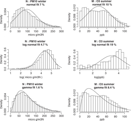
As discussed before, the definition of the statistical concepts to be used here does not depend on the statistical distributions of the data. However, the computation of the indexes becomes much simpler when normal or log-normal distributions are assumed. For simplicity, we will calculate the statistical indexes assuming log-normal distributions for all data. We explored the actual data distributions by fitting statistical models to the data. The results are shown in Table 2 and see also Fig. 3. The log-normal distribution fits the collected data better than ca. 20% relative quadratic error for all species except sulphur dioxide. We attribute this misfit to an unfortunate rounding procedure applied to the data by the network operators possibly due to the low absolute values currently measured in Santiago (less than ca. 5 ppbm annual average). Notice that the data are generally well described by other statistical models as it is the case of gamma distributions, but, to our knowledge, simple expressions for (1) in the multivariate gamma case are not known, although mutual information (7) and distance (8) can still be easily computed for arbitrary distributions. All in all, the assumption of log-normal distributions seems justified for all species except for SO₂.

Fig. 3 Example of some statistical fitting. PM₁₀ in winter for station N and O₃ for stations M for normal (top line), log-normal (middle line) and gamma (bottom line) fitting. The relative quadratic error is indicated on each case.

From the filtered data, we computed the ‘specificity’ and ‘representativity’ indexes according to their definitions (3) and (5) for each monitoring station. First, we consider a univariate analysis per species, per season, year-to-year and for all years (1997–2008). We then repeat this analysis considering a multivariate approach for all species at once. We use hourly averaged data. We explored other averaging windows finding similar results (not shown).

4.1. Univariate analysis

For species CO, O₃, PM₁₀ and SO₂ separately (univariate), we choose for the ‘representativity’ index calculation (see Section 2.2) background mean , where µ _ij are chosen such that exp µ _ij ≈0 (recall we work with the log of the data) and background covariance with , where is the j-th block of the full covariance matrix corresponding to the j-th species. Again, this choice is subject to improvement by considering other a priori information such as spatial distribution of pollutants and stations obtained by linear interpolation, kriging, dispersion models, and so on. The ‘specificity’ index calculation (see Section 2.1) does not need any background information.

Furthermore, we split the analysis by considering only summer (Dec, Jan, Feb), winter (Jun, Jul, Aug) or the whole year for all hourly data for the period 1997–2008. The resulting ‘specificity’ and ‘representativity’ indexes for the univariate case considering all data for the 1997–2008 period are illustrated for the summer and winter periods in Figs. 4 and 5. For all species and seasons, station M shows the highest ‘specificity’. This is consistent with the location of the station in a high-income area of the city where emissions patterns are different from elsewhere in Santiago and they consist of mostly residential sources and light duty vehicles (e.g. Gallardo et al., 2012b). Furthermore, this station is located at higher altitude (ca. 700 m a.s.l.) than other stations of the network in a relatively narrow canyon to the north-east of the basin. These characteristics make this station rather unique and thereby ‘specific’. Station El Bosque (Q) and other west located stations (O, P) are the second most specific stations at least with respect to sulphur dioxide in winter and PM₁₀ in summer. Around station Q there are industries including smaller smelters that co-exist with a low-income area of the city, which explains the specific behaviour in terms of sulphur dioxide.

Fig. 4 Specificity (left) and representativity (right) for the univariate case for CO, O₃, PM_10, and SO₂ for summer for seven stations during 1997–2008. The larger the circle, the larger the index.

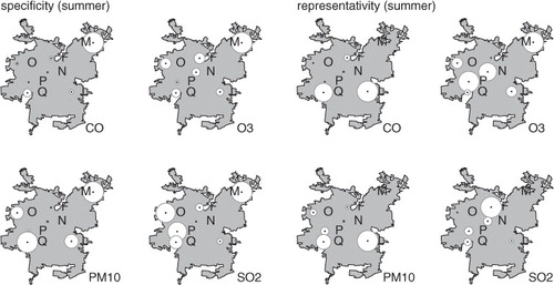
Fig. 5 Specificity (left) and representativity (right) for the univariate case for CO, O₃, PM₁₀ and SO₂ for winter for seven stations during 1997–2008. The larger the circle the larger the index.

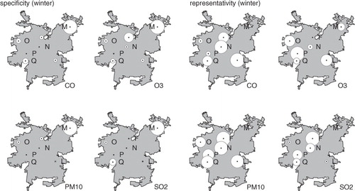
The ‘representativity’ index is linked, on the one hand, to the precision of the measurements (quantified by the inverse of the variance), and, on the other hand, by the magnitude of the measured values. Hence, in summer, ozone shows highest ‘representativity’ at M where magnitudes and variances are persistently large, and at P and N where magnitudes and variances are persistently small. Notice that M shows high ‘representativity’ only for ozone in summer when the signal's magnitude dominates over its lack of precision (large variance). Other species show no clear pattern in summer since the measured values have small magnitudes and large variances. In winter, the highest ‘representativity’ indexes for all species are found in downtown stations, mainly N and F, located in a relatively flat area of the Santiago basin. Here, signals show high magnitude and variance for tracers largely associated with mobile sources.

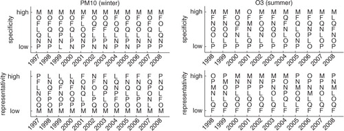
We also compute the evolution of the ‘specificity’ and ‘representativity’ indexes from year-to-year, performing the calculations for successive summers, winters and for every year. The results for PM₁₀ in winter and O₃ in summer are depicted in Fig. 6. Notice that, for PM₁₀, the north-eastern peripheral station M shows the highest ‘specificity’ for both species in all years whereas downtown stations display the highest ‘representativity’. Similar results are found for other species CO and SO₂ (not shown). The situation is only different for O₃ in summer: downtown stations and station M share high ‘representativity’ indexes. In other words, the classification is robust, stable in time and consistent with the east–west gradients in emissions and the east–west circulation pattern characteristic of Santiago. It is worth pointing out that these indexes can be viewed as dynamic indicators of the network since they continuously change according to each pollutant, temporal and spatial distribution of emissions and precursors, and circulation patterns. This could be relevant when using these indexes for analysing a network within the framework of defining long-term policies and curbing measures.

Fig. 6 Evolution of ‘specificity’ (upper panels) and ‘representativity’ (lower panels) indexes for PM₁₀ in winter and O₃ in summer respectively. See text for details.

4.2. Multivariate analysis

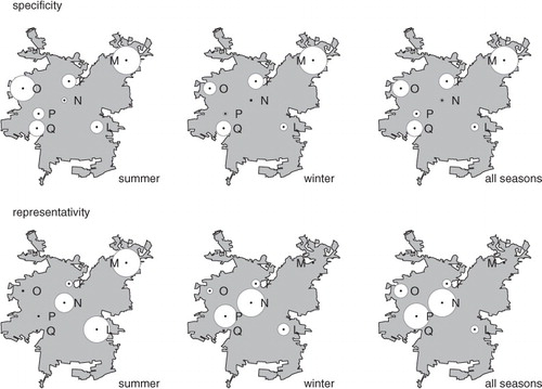
The corresponding results for the multivariate case are shown in Fig. 7. Again, station M has the highest ‘specificity’. In general, downtown stations show highest ‘representativity’ indexes in winter. In summer, stations L and M are displayed as most representative of the overall behaviour of the network. We attribute this to the fact that the most prominent summer pollutant is the photochemically driven ozone, which maximises in the afternoon hours in the easter-bound stations. In winter, changes in boundary layer height are primarily driven by solar radiation affecting the development of the mixing layer with nearly-collapsed conditions in nighttime that result in extremely high concentrations of particles and primary pollutants in the stations to the west of the basin (see Saide et al., 2011). Photochemical pollutants are also present in winter but to a lesser extent than in summer. Hence the ‘representativity’ of the stations is strongly modulated by emission and insolation cycles. Notice that station N, located in a relatively flat area of the basin, shows persistently a high ‘representativity’ index in the multivariate case. In this sense, this is the least expendable station of all contrary to what a pure mutual information analysis would suggest (e.g. Silva and Quiroz, 2003).

Fig. 7 Multivariate specificity (top) and representativity (bottom) indexes for simultaneously CO, O₃, PM₁₀ and SO₂ for hourly data for the period 1997–2008 separately for summer, winter and all seasons.

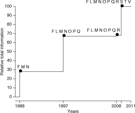
5. Evolution analysis

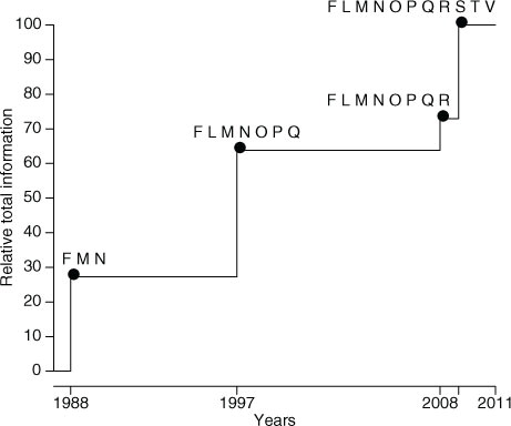
First, we analyse the evolution of the total information of the network by computing the information gaps given by (6) for the network by 1988 consisting of three stations (F, N and M), then considering seven stations when the largest expansion of the network occurred in 1997. We then estimate the changes due to the addition of station R, and finally we address the expansion to peripheral stations V, S and T by 2009. We do the same choice of background mean and covariances as in Section 4. The results are shown for fully inhalable particles in Fig. 8 using the hourly data of PM_2.5 from the network of 11 stations for the period 2009–2010. The increase in total information estimated for the network is roughly proportional to the number of monitoring stations added, and does not take into account their spatial distribution. This feature follows from the simple choice of a priori background mean and covariances. A different choice based on more sophisticated interpolation techniques such as kriging or air quality modelling (e.g. Wu and Bocquet, 2011) may improve the way in which the evolution of the network is quantified. This is beyond the scope of this study, but we give some insights about these techniques in the next sections.

Fig. 8 Evolution of total information content of the air quality monitoring network in Santiago since the late 1980s relative to the current situation, considering PM_2.5.

In order to have an idea of the influence of the choice of the a priori variables in the calculations we used a very simple interpolation technique [more precisely what is called the first step of Barnes interpolation, Barnes, 1964] as an alternative method to estimate the a priori mean and covariances B _i at each step of the evolution of the network. More precisely, from measurements z _k at points (x _k , y _k ) we infer measurements at site (x _i , y _i ) by the weighted mean

where L is a characteristic length related to the discretisation step δ. Using the data of the network corresponding to some given year, we interpolate values at other potential network sites and we can easily compute the corresponding a priori mean and covariances from the interpolated data. More precisely, if µ _k and Σ _kl are the mean at point (x _k , y _k ) and covariances between points (x _k , y _k ) and (x _l , y _l ) of the current network, the mean at point (x _i , y _i ) and covariances between points (x _i , y _i ) and (x _j , y _j ) of the interpolated network can be obtained by

From this we extract the background information and B _i . This is a simple and easy to implement method that takes into account the spatial distribution of the stations (see Fig. 9 computed with L=10,104 δ ²/π and δ=0.0133° in a 50×50 grid). Notice also that Barnes interpolation converges to the nearest neighbour interpolation for small values of L when it is compared with the domain size.

Fig. 9 Simulated interpolation of the measurements at some sites (×) from the available network (•) using Barnes interpolation (here for some typical log concentrations of PM₁₀ in greyscale, lighter=higher). To localise, we put 12 phantom zero measurement stations around the boundary. This allows to better estimate the a priori mean and covariances B _i for the evolution of network total information taking into account the spatial distribution.

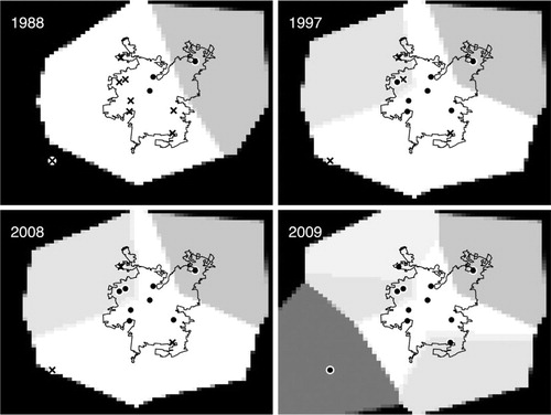
To simplify the analysis, in a first approximation we can neglect covariances and we compute the new mean and just the new variances given by . With this, we can obtain the information gaps directly using (2) where µ ₁, Σ₁ and µ ₀, Σ₀ correspond to the mean and variances estimated by interpolation before and after a change according to the new network distribution. As expected, we can see from Fig. 10, when compared to Fig. 8 that the addition of station R to the network has only a small influence on the total PM_2.5 information since the new station R was very close to the already existing station O in the previous network. A similar situation can be verified for PM₁₀ (not shown).

Fig. 10 Evolution of total information content of the air quality monitoring network in Santiago since the late 1980s relative to the current situation, considering PM_2.5 using Barnes interpolation a priori information.

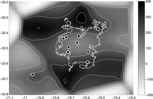
Further analysis concerning the choice of a priori information without neglecting covariances requires applying other interpolation techniques such as kriging or dispersion modelling, which is beyond the scope of this work. We are currently working on this as this provides a way to select new observational sites.

For example, in Fig. 11, we see the total information gain obtained at each point of a spatial grid surrounding the stations, if we add a new virtual station with Barnes's interpolated measurements at this point, and we recompute the total information after considering this new station. So we could try to add stations in the regions with highest information gain. Of course, these type of analysis are limited, and the use of more sophisticated dispersion and chemistry modelling is needed, so this should be the subject of further study.

Fig. 11 Information gain map. At each point, the difference in information gain obtained by comparison of the total information gain of the original network and the total information gain obtained for a new network after adding a new station at this point with Barnes's interpolated values is indicated.

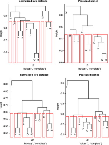
6. Clustering analysis

We perform hierarchical clustering analysis of the network for 11 stations of PM_2.5 and PM₁₀ hourly data in 2009–2010 and O₃ hourly data in 2009 using the normalised information distance defined in (8) without any normality assumption. The results of the clustering are depicted in Fig. 12. We select six clusters that are the same for particulate matter: M, T, Q, [L, S], [F, N], [V, P, O, R] and different for ozone: M, T, [L, S], [F, Q], [N, P], [V, O, R]. Similar results for particulate matter can be obtained by using Pearson's distance (see Section 2.4), after taking the logarithm of data, but they are slightly different for ozone. This is not surprising since both distances are related in the normal case, and from Table 2, we see that the log-normal adjustment is better for particulate matter than for ozone. This example illustrates that information distance is more robust than Pearson distance for other data distributions. Notice that we also checked k-means clustering analysis for k=5 or 6 clusters with similar results.

Fig. 12 Hierarchical clustering following the (not normal) normalised information distance (left column) defined in (8) compared with the Pearson correlation function (right column) for PM_2.5 (top line) and O₃ (bottom line).

Primarily, these clusters reflect the main circulation pattern of the Santiago basin, namely a thermally driven circulation with south-westerly winds peaking in the afternoon and north-easterly winds peaking in the night. Also, they respond to the east–west gradients in emissions of primary pollutants. This is clear in the case of the PM_2.5 winter clustering that is dominated by the distribution of traffic sources (e.g. Gallardo et al., 2012b). In the case of the summer ozone cluster, east–west differences are more smeared out due to the more intensive mixing. All in all, the main distinction is between the eastern and western bounds of the basin for all clusters, independently of season, species and distance considered. This pattern has been described elsewhere by various authors, for example, Gallardo et al. (2002); Gramsch et al. (2006); Saide et al. (2011). Also, a common feature for all clusters is that stations M and T show a very specific and distinct behaviour. M is located in a high-income area of the city where emissions patterns are different from elsewhere in Santiago and they consist of mostly residential sources and light duty vehicles (e.g. Gallardo et al., 2012b). Furthermore, this station is located at higher altitude (ca. 700 m a.s.l.) than other stations of the network in a relatively narrow canyon to the north-east of the basin. T, on the contrary, is the only suburban/rural station located to the west of the basin, at its south-westerly outflow. This analysis confirms the utility and importance of clustering analysis in the detection of common spatial patterns (see Ignaccolo et al., 2008).

7. Conclusions and outlook

We have introduced statistical concepts to quantify the information content as well as what we call the ‘representativity’ and ‘specificity’ indexes of air quality stations in a monitoring network. These indexes stem from information theory concepts, in particular mutual information and information gain. We emphasize that these indexes must be used concurrently if one wants to address the ‘goodness’ of monitoring network, in accordance with the international community agreement of multi-objective network design, and that looking at only one of them may lead to erroneous conclusions. Finally, we use clustering techniques to identify groups of stations with similar characteristics. Furthermore, we show how to assess the temporal evolution of a network in terms of information content. We analysed 14 yr of data collected by the air quality monitoring network in Santiago de Chile to illustrate the use of the information indexes.

The ‘representativity’ and ‘specificity’ indexes are shown to be robust and consistent with known emission and circulation patterns in Santiago de Chile, namely persistent east–west gradients in emission patterns and the thermally driven circulation with up-slope winds in the afternoon and down-slope winds during nighttime. We find that measurements in downtown stations, located in a relatively flat area of the Santiago basin, generally show, for all seasons and species, high ‘representativity’ and low ‘specificity’, whereas the contrary is found for a station located in a canyon to the east of the basin. Clustering results corroborate the characteristics identified using the indexes derived from information theory.

Regarding the evolution of a network, we showed how to quantify the corresponding changes in information content. We found that in the case of Santiago, the current network configuration is four times more informative than the initial configuration in the late 1980s, and twice as much as that of 1997. If we choose the simplest background a priori information, the changes in information content are roughly proportional to the changes in number of stations and this follows from a very simple choice for estimating the background mean and covariances that does not consider the spatial distribution of the stations. This can be avoided by using kriging or other interpolation techniques to better address the changes in information content linked to the spatial distribution of the monitoring stations in a network as illustrated by means of Barnes’ interpolation in Figs. (9–11). What seems important is that the indexes presented here, if used in combination with adequate interpolation tools, may be used to obtain the optimal location of new stations by maximising the total information of the network.

All in all, the statistical indexes presented here provide an objective manner to analyse monitoring networks in terms of information content, their evolution, and if used in combination with adequate interpolation techniques, a way to infer best locations for new stations.

Acknowledgements

This work is being carried out with the aid of a grant from the Inter-American Institute for Global Change Research (IAI) CRN II 2017 which is supported by the US NSF Grant GEO-0452325 and CONICYT/FONDAP/15110009. A. Osses also acknowledges Fondecyt 1110290 and ACT-1106 ACPA grants. Discussions with Prof. M. Bocquet are much appreciated.

References

- Ainslie B , Reuten C , Steyn D. G , Le N. D , Zidek J. V . Application of an entropy-based Bayesian optimization technique to the redesign of an existing monitoring network for single air pollutants. J. Environ. Manage. 2009; 90(8): 2715–2729.
- Barnes S. L . A technique for maximizing details in numerical weather-map analysis. J. Appl. Meteorol. 1964; 3(4): 396–409.
- Bocquet M . Construction optimale de réseaux de mesures: application à la suveillance des polluants aériens (Optimal design of observational networks: application to air-quality monitoring). ParisTech/ENSTA lecture notes. 2009. Version 1.13, Paris. Available online at http://cerea.enpc.fr/HomePages/bocquet/Doc/network-design-mb.pdf .
- Caselton W , Zidek J . Optimal monitoring network designs. Stat. Probab. Lett. 1984; 2: 223–227.
- Chatelain F , Tourneret J.-Y , Inglada J , Ferrari A . Change detection in multisensor SAR images using bivariate gamma distributions. IEEE Trans. Image Process. 2008; 16(7): 249–258.
- Chow J , Engelbrecht J , Watson J , Wilson W , Frank N , co-authors . Designing monitoring networks to represent outdoor human exposure. Chemosphere. 2002; 49: 961–978.
- Coeurjolly J.-F , Drouilhet R , Robineau J.-F . Normalized information-based divergences. Probl. Peredachi. Inf. 2007; 43(3): 3–27.
- Elkamel A , Fatehifar E , Taheri M , Al-Rashidi M. S , Lohi A . A heuristic optimization approach for air quality monitoring network design with the simultaneous consideration of multiple pollutants. J. Environ. Manage. 2008; 88: 507–516.
- Gallardo L , Escribano J , Dawidowski L , Rojas N. J , Andrade M. F , Osses M . Evaluation of vehicle emission inventories for carbon monoxide and nitrogen oxides for Bogotá, Buenos Aires, Santiago, and São Paulo. Atmos. Environ. 2012b; 47: 12–19.
- Gallardo L , Olivares G , Langner J , Aarhus B . Coastal lows and sulfur air pollution in Central Chile. Atmos. Environ. 2002; 36: 315–330.
- Gallardo L , Alonso M , Andrade M. F , Dawidowsky L , Gomez D , co-authors . Zhu T , Parrish D , Gauss M , Doherty S , Lawrence M , co-authors . South American megacities. In: The Impacts of Megacities on Air Quality and Climate Change: An IGAC Perspective. 2012a; , Switzerland: Geneva. 141–171. IGAC/WMO book and report.
- Garreaud R. D , Ruttlant J , Fuenzalida H . Coastal lows along the subtropical west coast of South America: mean structure and evolution. Mon. Weather Rev. 2002; 130: 75–88.
- Gramsch E , Cereceda-Balic F , Oyola P , Von Baer D . Examination of pollution trends in Santiago de Chile with cluster analysis of PM10 and ozone data. Atmos. Environ. 2006; 40: 5464–5475.
- Haas T. C . Redesigning continental-scale monitoring networks. Atmos. Environ. 1992; 26A: 3323–3333.
- Ignaccolo R , Ghigo S , Giovenali E . Analysis of air quality monitoring networks by functional clustering. Environmetrics. 2008; 19: 672–686.
- Kullback S . Information Theory and Statistics. 1959; New York: Wiley.
- Le N. D , Zidek J. V . Statistical Analysis of Environmental Space-Time Processes. New York: Springer.
- Nielsen F , Nock R . Entropies and cross-entropies of exponential families. In: ICIP'10 – International Conference on Image Processing. 2010; Hong Kong, China: IEEE SP Press. 3621–3624.
- Pérez-Abreu V , Rodríguez J . Index effectiveness of a multivariate environmental monitoring network. Envirometrics. 1996; 7: 489–501.
- Pesch R , Schröder W , Dieffenbach-Fries H , Genßler L , Kleppin L . Improving the design of environmental monitoring networks. Case study on the heavy metals in mosses survey in Germany. Ecol. Informat. 2008; 3: 111–121.
- Ruiz-Cárdenas R , Ferreira M , Schmidt A . Stochastic search algorithms for optimal design of monitoring networks. Environmetrics. 2010; 21: 102–112.
- Ruiz-Cárdenas R , Ferreira M , Schmidt A . Evolutionary Markov chain Monte Carlo algorithms for optimal monitoring network designs. Stat. Meth. 2012; 9(1–2): 185–194.
- Saide P , Carmichael G , Spak S , Gallardo L , Mena M , co-authors . Forecasting urban PM10 and PM2.5 pollution episodes in very stable nocturnal conditions and complex terrain using WRF-Chem CO tracer model. Atmos. Environ. 2011; 45: 2769–2780.
- Saunier O , Bocquet M , Mathieu A , Isnard O . Model reduction via principal component truncation for the optimal design of atmospheric monitoring networks. Atmos. Environ. 2011; 43: 4940–4950.
- Shannon C . A mathematical theory of communication. Bell. Syst. Tech. J. 1948; 27(3): 379–423.
- Silva C , Quiroz A . Optimization of the atmospheric pollution monitoring network at Santiago de Chile. Bell. Syst. Tech. J. 27, 379–423 . 2003; 623–656.
- Wu L , Bocquet M . Optimal redistribution of the background ozone monitoring stations over France. Atmos. Environ. 2011; 45(3): 772–783.
- Zhu T , Parrish D , Gauss M , Doherty S , Lawrence M , co-authors . The Impacts of Megacities on Air Quality and Climate Change: An IGAC Perspective. 2012. IGAC/WMO book/report published on line in October 2012. Online at: http://www.wmo.int/pages/prog/arep/gaw/documents/GAW_205_DRAFT_13_SEPT.pdf .
- Zidek J. V , Sun W , Le N. D . Designing and integrating composite networks for monitoring multivariate Gaussian pollution fields. J. Roy. Stat. Soc. C. 2000; 49(1): 63–79.
- Zidek J. V , Zimmerman D. L , Gelfand A. E , Diggle P. J , Fuentes M , Guttorp P . Chapter 10. Monitoring network design. In: Handbook of Spatial Statistics. 2010; , New York: CRC Press, Taylor and Francis Group,.