Microphysical imprint of entrainment in warm cumulus

Abstract

We analyse the cloud microphysical response to entrainment mixing in warm cumulus clouds observed from the CIRPAS Twin Otter during the GoMACCS field campaign near Houston, Texas, in summer 2006. Cloud drop size distributions and cloud liquid water contents from the Artium Flight phase-Doppler interferometer in conjunction with meteorological observations are used to investigate the degree to which inhomogeneous versus homogeneous mixing is preferred as a function of height above cloud base, distance from cloud edge and aerosol concentration. Using four complete days of data with 101 cloud penetrations (minimum 300 m in length), we find that inhomogeneous mixing primarily explains liquid water variability in these clouds. Furthermore, we show that there is a tendency for mixing to be more homogeneous towards the cloud top, which we attribute to the combination of increased turbulent kinetic energy and cloud drop size with altitude which together cause the Damköhler number to increase by a factor of between 10 and 30 from cloud base to cloud top. We also find that cloud edges appear to be air from cloud centres that have been diluted solely through inhomogeneous mixing. Theory predicts the potential for aerosol to affect mixing type via changes in drop size over the range of aerosol concentrations experienced (moderately polluted rural sites to highly polluted urban sites). However, the observations, while consistent with this hypothesis, do not show a statistically significant effect of aerosol on mixing type.

• inhomogeneous mixing
• homogeneous mixing
• GoMACCS
• phase-Doppler interferometer
• cloud microphysics

1. Introduction

Entrainment is the process by which sub-saturated air surrounding a cumulus cloud is drawn into the cloud due to the (turbulent) motions of the cloudy air. The result of entrainment is a dilution of both total water and liquid water, and thus this process is important in governing the evolution of clouds.

The mixing of the sub-saturated air with cloudy air, and the evaporation of liquid water to bring this air to water saturation, comprise the cloud response to entrainment (hereafter termed entrainment mixing or just mixing). If sufficient dry air is entrained, all the liquid water can evaporate causing complete dissipation of a cloudy volume. If, however, there is an excess of liquid water over that required bringing the entrained air to saturation, then the drop population remaining in the cloud volume has been altered due to entrainment. The change in cloud microphysical properties due to entrainment has been the subject of numerous studies due to its relevance to key processes such as precipitation and short-wave reflectance (e.g. Baker et al., 1980; Paluch and Baumgardner, 1989; Su et al., 1998; Lasher-Trapp et al., 2005; Derkson et al., 2009). In this study, we focus on the following questions relating to the microphysical response of warm, non-precipitating Cu to entrainment: (1) How does entrainment mixing affect cloud drop size distributions? (2) What does this mixing depend on? and (3) Can aerosol influence the effects of entrainment mixing? The third question is motivated by interest in the effects of aerosol on the formation and evolution of cumulus clouds.

Many processes within cumulus clouds depend on their microphysical properties. For example, precipitation and radiative processes depend on the total cloud drop number concentration (N) and the mean and shape of the drop size distribution (DSD) for the entire cloud drop population. Entrainment modifies microphysical properties by decreasing cloud liquid water content (LWC). Since , where N is cloud drop concentration and D _v is mean volume diameter, the loss of LWC can occur via (1) the decrease of N, termed inhomogeneous mixing (e.g. Latham and Reed, 1977; Hill and Choularton, 1985; Jensen et al., 1985; Lasher-Trapp et al., 2005), (2) a decrease in D _v, termed homogeneous mixing (e.g. Baker et al., 1980; Telford et al., 1984; Jensen et al., 1985; Burnet and Brenguier, 2007), or (3) a combination of both, which represents a ‘mixture’ of these two end-member types of mixing (Lasher-Trapp et al., 2005). During homogeneous mixing, after being exposed to sub-saturated air, all drops partially evaporate to re-establish saturation, causing the DSD to shift to smaller diameters (the very smallest drops, a few µm in size, may completely evaporate). During inhomogeneous mixing, a subset of drops completely evaporates to re-establish saturation, causing N to decrease, but the shape of the DSD remains the same. The ratio of the time scale it takes for a drop to evaporate, τ _evap, to the time scale required to mix the cloudy and cloud-free air, τ _mix (Baker et al., 1984), is believed to control the cloud microphysical response to entrainment, that is, the location in the continuum between homogeneous and inhomogeneous mixing. In the limit, homogeneous mixing occurs when τ _evap >> τ _mix whereby all cloud drops are exposed to the same sub-saturation after complete mixing of the cloud and cloud-free parcels. Perfectly inhomogeneous mixing occurs when the converse is true, that is, τ _mix >> τ _evap whereby drops adjacent to sub-saturated regions completely evaporate rapidly while the remaining drops are completely unaffected. Following Baker et al. (1984), the time scale for the evaporation of a single drop is given by:1

where k is a function of temperature and pressure and RH represents the relative humidity. We see that τ _evap depends on the characteristic drop diameter D. One potential consequence is that τ _evap will increase with cloud height as drops grow larger by condensation, all other factors (such as environmental RH and turbulence) being equal. Also, more polluted clouds, with smaller drops, may cause τ _evap to decrease and shift mixing towards the inhomogeneous end-member (again, all other factors being equal). Lehmann et al. (2009) describe a related time scale, one for the clear air, without a cloud present, to return to saturation. This phase-relaxation time scale depends on the rate of evaporation of the entire population of drops, which we re-write as:2

As LWC increases, τ _phase decreases. For fixed LWC, as diameter increases, surface area decreases and therefore τ _phase increases. Which one of these reaction time scales is more appropriate depends on the microphysical context, and in some cases when τ _phase≈τ _evap, both are smaller than the time required to restore saturation (Lehmann et al., 2009). The turbulent mixing time scale is given by:3

Where l is a mixing length scale and ɛ, the energy dissipation rate. Regions of the cloud with stronger turbulence should have smaller τ _mix and hence may shift mixing towards the homogeneous end-member. The Damköhler number, Da, can be defined as the ratio of the mixing time scale to that for phase change, that is:4

where we have dropped the RH or LWC term for clarity. No matter whether τ _evap (i.e. single drop) or τ _phase (i.e. drop population) is used to set the evaporation time scale, the time scale can be written as proportional to D ² (although the assumptions are different). If Da is large, inhomogeneous mixing is favoured, while homogeneous mixing is favoured for smaller Da. Changes in ɛ and/or D are, therefore, predicted to change the nature of mixing in clouds.

In reality, the microphysical response to sub-saturated air is likely to be much more complex. Cumulus clouds are spatially and temporally variable, and mixing occurs across a range of scales and changes to the DSD as a result of mixing are highly variable (Bewley and Lasher-Trapp, 2011). Thus no single drop diameter, entrained air relative humidity, LWC, mixing length scale or energy dissipation rate is likely to be appropriate for computing these time scales, even within a single cumulus cloud. For example, Lehmann et al. (2009) show that variations in ɛ and τ _mix/τ _phase by factors as large as 10³ and 10, respectively, can occur within individual clouds. This suggests that mixing can have different character within the same cloud. Some cloudy regions may also have experienced multiple dilution events, each potentially of different character. Lastly, the turbulent transport of cloud drops will have a tendency to homogenise DSDs within a cloud, such that the signature of a ‘pure’ entrainment event would be lost after some time.

The goal of this work is to determine how and why the cloud microphysical response to entrainment mixing may vary in shallow, warm non-precipitating continental cumuli sampled during the Gulf of Mexico Atmospheric Composition and Climate Study (GoMACCS). We emphasise that our observations record a snapshot of each sampled cloud; thus, we are observing the net effect of entrainment mixing on the microphysical properties of that cloud. We have no way of knowing the history of any given air parcel; thus, we cannot elucidate the exact processes that led to the instantaneous microphysical state captured by our observations. A summary of the study and the meteorological conditions are presented in section 2. Section 3 describes the microphysical mixing diagram used for this study. Section 4 examines mixing processes using a multi-day, full-flight comparison of four flights including two rural (‘lower pollution’) and two urban (‘higher pollution’) conditions. Discussion of results and conclusions are presented in section 5.

2. Experiment and meteorological conditions

GoMACCS occurred in the vicinity of Houston, Texas, in August and September of 2006. These data represent a set of statistically sampled scattered continental cumuli under aerosol conditions ranging from remote continental to highly polluted. The Center for Interdisciplinary Remotely-Piloted Aircraft Studies’ (CIRPAS) Twin Otter aircraft was equipped with standard meteorological instrumentation for the measurement of temperature (T), dew point (T _d) and pressure (P) with other quantities derived as needed (see Table 1 of Lu et al. (2008) for a detailed description of the instrument payload). In- and out-of-cloud T, T _d and P are used in the calculation of mixing line curves plotted on mixing diagrams, described in detail in the following section. As noted by Lehmann et al. (2009) and others, temperature probes are often affected by wetting, such that during cloud transects the sensor measurements would be biased until the condensate evaporates. For GoMACCS, temperature measurements are obtained from a Rosemount 102 AL (Friehe and Khelif, 1992), with an absolute uncertainty of ±0.5°C and a response time of 0.02 s. Our temperature data are averaged to 1 Hz, and we do not see evidence of the wetting effect as seen with ultrafast thermometers used by Lehmann et al. (2009) based on comparisons of T entering and departing clouds. Measurements from two condensation particle counters, TSI models 3010 and 3025 (measuring dry aerosol number concentration greater than 10 nm and 3 nm, respectively) are used for determining aerosol regimes based on the study by Lu et al. (2008). The Passive Cavity Aerosol Spectrometer (PCASP), with its heaters running to dry all particles for particles 0.1–3.0 µm, is also used for this purpose. The Artium Flight phase-Doppler interferometer (Chuang et al., 2008) (F-PDI) is used for cloud microphysical measurements (2<D<100 µm) and F-PDI derived LWCs are used to identify in-cloud samples (LWC>0.01 g m⁻³). F-PDI data are chosen for in-cloud identification due to the ability of the F-PDI to detect large numbers of cloud droplets without coincidence effects (see Chuang et al., 2008 for a more detailed description of F-PDI limitations and capabilities). A combination of F-PDI and data from the Cloud Imaging Probe (CIP) component of the Cloud, Aerosol and Precipitation Spectrometer Probe (Baumgardner et al. (2001), 15<D<1550 µm) is used to detect drizzle (D >50 µm) and limit our analysis to non-precipitating clouds.

Table 1 Summary of cloud properties for clouds>300 m in width. Maximum cloud drop number concentrations and leg mean N _aerosol (#/cm⁻³) and N _acc (#/cm⁻³), one standard deviation in parenthesis, are from Table 2 of (Lu et al., 2008). The (Lu et al., 2008) are for full legs and have not been sorted for clouds>300 m in width. They are included for reference only. Two values are reported for L1 corresponding to two separate UTC time periods. Though (Lu et al., 2008) reports high leg mean N _aerosol for L2, the large standard deviation is the result of sampling a power plant plume (17:17 to 18:00 UTC) during an otherwise relatively clean flight. Values for average PDI cloud drop number concentration (CDNC) include data from all non-precipitating clouds greater than 300 m in width. For L2, two clouds sampled had peak CDNC values greater than 1000. With these two clouds excluded the maximum PDI CDNC is 983 cm⁻³

	L1	H1	L2	H2
Date	2006-Aug-26	2006-Sept-08	2006-Sept-11	2006-Sept-15
Flight Number	RF 5	RF 17	RF 19	RF 22
UTC for cloud sampling	1415–1717	1832–2000	1600–1718	1701–1754
# of clouds>300 m in width	24	24	37	16
Minimum cloud base height (m)	730	1490	1290	1150
Maximum cloud top height (m)	2130	2430	3070	2750
Cloud thickness (m)	1390	950	1780	1610
Average true air speed in cloud (m/s)	60.5±1.7	62.5±2.4	61.0±2.6	60.6±2.7
Average cloud width (m)	672	725	659	642
Average PDI cloud drop number concentration, (dN/dlogDp)	1570±350	2150±290	1960±510	1850±480
Mean PDI cloud drop number (N d)	250±150	640±390	330±290	260±157
Observed cloud top LWC (g/m^3)	1.15±1.25	0.66±0.68	0.55±0.53	1.43±1.20
Adiabatic cloud top LWC (g/m^3)	4.87	2.74	5.04	4.62
Leg mean Naerosol (#/cm^−3)	1884 (347); 1408 (506)	7496 (2633)	11500 (9051)	3355 (576)
Leg mean Nacc (#/cm^−3)	429 (70); 437 (49)	1582 (215)	595 (129); 595 (129)	903 (165)

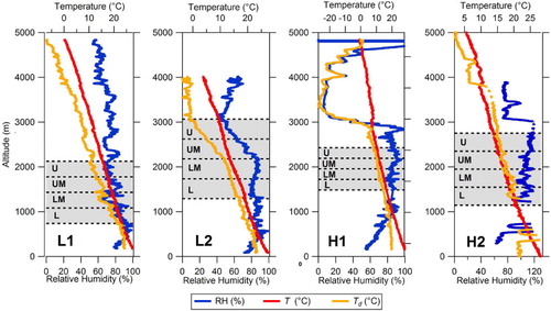
Soundings of T, T _d and RH taken during clear-air spirals before or after cloud sampling on the four days used in this study are shown in Fig. 1 along with the average height of cloud base and cloud top for each flight. Cloud base and cloud top heights are defined as the lowest level and highest level at which clouds were sampled for each day, as described by CIRPAS pilots and the on-board mission scientist. During any particular flight cloud base remained fairly constant varying, on average, by±60 m based on pilot accounts. We report altitude-dependent results using four different cloud regions, denoted lower, lower middle, upper middle, and upper. These quartile regions are determined as the bottom 25%, 25–50%, 50–75% and upper 25% of altitudes for each flight, as illustrated in Fig. 1, regardless of their absolute altitude. Use of normalised cloud height is common for comparison among different cloud cases (Jiang et al., 2006; Lu et al., 2008; Small et al., 2009). We note that on any given day, cloud penetrations are not evenly distributed among these different levels, and on some days, there may be no data at all from one region (e.g. lower middle) while another region was very well sampled.

Fig. 1 Out-of-cloud atmospheric soundings. Vertical soundings for four full flights L1 (2006-Aug-26), L2 (2006-Sept-11), H1 (2006-Sept-08) and H2 (2006-Sept-15). Note that RH measurement problems occurred during large portions of the sounding for H2 (i.e. values above 100%). Grey shaded areas represent cloud layers (from lowest observed cloud base to highest observed cloud top) for each research flight. Approximate altitudes for cloud regions, lower (L), lower middle (LM), upper middle (UM) and upper (U) for each flight are separated by dotted lines.

2.1. Statistical sampling of cumulus fields

For this study we choose to use two lower pollution flights, denoted L1 (2006-Aug-26) and L2 (2006-Sept-11) and two higher pollution flights denoted H1 (2006-Sept-08) and H2 (2006-Sept-15) out of the 22 GoMACCS research flights. For each flight, sampling of cumulus fields occurred by selecting closest reasonable cloud targets such that the data consists of an unbiased sample of cloud microphysical and dynamical properties over a large geographic region under similar meteorological conditions. We choose the two most-polluted and two least-polluted flights, with satisfactory cloud sampling, in order to maximise the aerosol concentration contrast. All flight data have been filtered such that only non-precipitating cumulus are included in the analysis. Filtering is critical since the mixing diagram is most useful under conditions of minimal collision-coalescence as discussed below. We also filter for clouds greater than 300 m in width. Over all flights, mean and σ of cloud width are 680 and 337 m, respectively. Detailed information regarding each flight is available in Table 1. Note that the ultrafine aerosol concentration during L2, classified as a lower pollution day, is elevated. This was due to the aircraft sampling in the vicinity of a coal-burning power plant for part of the flight. The portion of the flight traversing the power plant plume, as specified by the pilot and mission scientist and indicated by particle concentration values significantly above background, is excluded from this analysis such that only clean conditions are included in the calculations. Our classification of lower or higher pollution is based on concentrations of total aerosol (measured by the TSI 3010), N _tot, and accumulation-mode aerosol (measured by the PCASP), N _acc, found in Table 2 of Lu et al. (2008). For L2, N _acc was ~600 cm⁻³ while N _tot was ~2500 cm⁻³, once the power plant-influenced data were removed from the ultrafine aerosol record (see Table 1 for more information). Flight paths for L1, L2, H1 and H2 days covered similar geographic areas; thus, surface characteristics are likely to be similar.

Table 2 Full flight Wilcoxon ranked-sum test results for α, α weighted D _v ³/D _va ³ values and α weighted N/N _a for full clouds. Each cloud region is compared to the others; that is, all of the D _v ³/D _va ³ data included in the Lower region of cloud is compared to all of the D _v ³/D _va ³ data in the Lower-Middle region of cloud and so on. Comparisons that result in statistically significant values, with p<0.01 are boldfaced. Six of the seven statistically significant comparisons are such that D _v ³/D _va ³ decreases with increasing height. A lack of data hampers comparisons of the Lower-Middle region with other levels for H2, and of the Upper Middle region with other levels for L2

	α		Dv^3/Dva^3		N/Na
	p	Trend with Alt.	p	Trend with Alt.	p	Trend with Alt.
L1 (2006-Aug-26)
Lower Middle–Upper Middle	0.8484	↓	0.5663	↓	0.9032	↓
Upper Middle–Upper	0.6639	↑	0.0037	↑	0.1808	↑
Lower Middle–Upper	0.6143	↑	0.0735	↑	0.4342	↓
H1 (2006-Sept-08)
Upper Middle–Upper	0.4979	↓	0.4549	↓	0.8484	↓
L2 (2006-Sept-11)
Lower–Lower Middle	0.2891	↑	0.3945	↓	0.0157	↑
Lower Middle–Upper Middle	0.0420	↑	0.0037	↓	0.0010	↑
Upper Middle–Upper	0.0208	↓	0.1492	↑	0.1492	↓
Lower Middle–Upper	0.4761	↓	0.0013	↓	0.0010	↓
Lower–Upper	0.5430	↑	0.0010	↓	0.1698	↓
Lower–Upper Middle	0.0420	↓	0.0078	↓	0.4140	↑
H2 (2006-Sept-15)
Lower–Lower Middle	0.1592	↓	0.3219	↓	0.4761	↓
Lower Middle–Upper Middle	0.4140	↑	0.0064	↓	0.0325	↑
Upper Middle–Upper	0.9584	↑	0.4761	↓	0.0386	↑
Lower Middle–Upper	0.2047	↑	0.0071	↓	0.0010	↑
Lower–Upper	0.5901	↑	0.5202	↓	0.0208	↑
Lower–Upper Middle	0.7943	↓	0.4242	↓	0.8757	↓

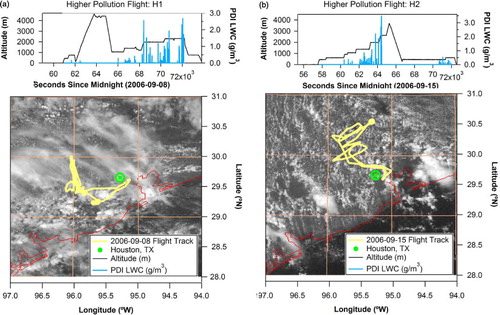
Figures 2 and 3 show the four flight paths overlaid over a 1-km resolution GOES-East image taken during the middle portion of each flight. Macrophysical properties of clouds, such as cloud width, organisation and cloud top, are similar for all days regardless of aerosol concentration. Cloud size is also similar for all days with average widths of ~700 m (Table 1). For L1 and H2, the clouds appear to be organised along the mean wind (S-SE) and in a more random configuration during L2 and H1. A notable difference is that H1 had an overlying layer of cirrus in conjunction with an overlying dry layer (see Fig. 1) for much of the flight. This cirrus may have limited cumulus cloud development during this flight and resulting in thinner clouds for H1 (950 m) as compared to other flights (see Table 1).

Fig. 2 Research flight paths and GOES-East imagery for lower pollution days. Flight paths and altitude and LWC profiles for (a) L1 and 1-km GOES-East image at 1600 UTC and (b) L2 and the 1-km GOES-East image at 1700 UTC. The coastline is represented by the red line and the location of Houston, Texas, is shown for reference.

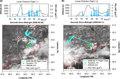
Fig. 3 Research flight paths and GOES-East imagery for higher pollution days. Flight paths and altitude and LWC profiles for (a) H1 and the 1-km GOES-East image at 1900 and (b) H2 and the 1-km GOES-East image at 1730. The coastline is represented by the red line and the location of Houston, Texas, is shown for reference.

3. The mixing diagram

In order to study the cloud microphysical response to entrainment mixing, we use a mixing diagram (Burnet and Brenguier, 2007) as shown schematically in Fig. 4. The x-axis is the droplet number concentration normalised by its adiabatic value, N/N_a, and the y-axis is given by the cube of the mean volume diameter (D_v) normalised by its adiabatic value, , where is defined as:5

Fig. 4 Entrainment mixing diagram. Dashed lines represent the relationship between and N/N_a during homogeneous mixing of air at various relative humidities. Bold dashed lines highlight mixing with air of 100 and 80% (the average ambient RH for the four flights included in study). The 100% RH homogeneous mixing line is the same as the inhomogeneous mixing line. Dash-dotted lines represent the dilution ratio, α=LWC/LWC_a, where LWC_a is the adiabatic liquid water content. α is plotted at 0.1 intervals from α=1 to α=0.1. Values in the region of the shaded oval may result if the chosen reference N_a is too small for a particular cloud sample or if collision-coalescence is active. Note that collision-coalescence cannot yield samples with α>1, but this could happen if drops sediment into a sample volume from higher parts of cloud.

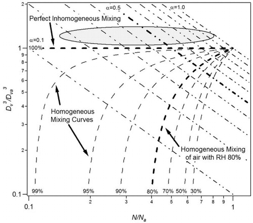
where ρ_a is the density of the air, ρ_w is the density of water, q_T is the observed specific liquid water mixing ratio and N is the droplet number concentration. The cube of the adiabatic mean volume diameter, , is calculated using q_Ta, the adiabatic liquid water mixing ratio for each altitude level, and the adiabatic droplet number concentration, N_a. For this study, N_a is the average of the top 2% of 1-s droplet number concentration observations for each day and D_va, is the average adiabatic mean volume diameter for the specified altitude swath. As noted by Lehmann et al. (2009), for both axes, the normalisation accounts for variations in cloud base height and/or changes in sampling altitudes which is ideal for our multi-cloud multi-flight analysis.

If an air parcel experiences inhomogeneous mixing as described by Baker et al., 1980, D_v stays constant during dilution and evaporation while N is diminished. Thus, the measured values will form a horizontal line with constant. For the homogeneous case, the mixing in of dry air (with a specific relative humidity) occurs quickly, resulting in a more thorough intermingling of cloudy and clear air such that all the cloud drops experience the same relative humidity as they interact. For example, during an idealised homogeneous mixing event with cloud-free air at 80% RH, all drops in the ‘mixed parcel’ would experience dry air of 80% RH. On the mixing diagram (Fig. 4), the properties of this idealised ‘mixed parcel’ would fall along the 80% homogeneous mixing line. Addition of cloud-free air causes N to decrease by dilution. At the same time, all the drops partially evaporate; that is, D_v decreases, in order to bring the entrained air up to saturation. Thus, all of the dashed lines indicating homogeneous mixing at different RH decrease along both the x- and y-axis from the adiabatic reference point. Note that homogeneous mixing of air with RH=100% (but that is free of drops) causes only dilution and no reduction in drop size and, therefore, is indistinguishable from inhomogeneous mixing where some of the droplets fully evaporate while others remain unaffected. However, the homogeneous mixing of air with RH<100% will result in both dilution of cloud drop number and a reduction in drop size which is distinguishable from inhomogeneous mixing. We further define the LWC dilution ratio, or adiabaticity, which is defined as:6

where q_l is the liquid water mixing ratio (g/kg) and q_la is the adiabatic liquid water mixing ratio (g/kg). It is plotted at 0.1 intervals from α=0.1 to α=1. Data with both N/N_a and values close to 1 are close to adiabatic. The relationship between observations and α indicates the amount dilution. For example, observations with α=0.1 are more diluted than those with α=1.0.

There are inherent uncertainties and biases in the measurements, which result in limitations when using these mixing diagrams. The measured values of N_a and hence the inferred values of D_va can be affected by several uncertainties and assumptions (Lehmann et al., 2009): fluctuations in cloud base; fluctuations in updraft velocity and aerosol conditions among clouds; the assumption that maximum observed cloud drop number concentration (CDNC) is the true adiabatic value; the assumption that no additional activation of cloud drops occurs above cloud base; and the potential underestimation of CDNC as a result of horizontal averaging of heterogeneous cloud–cloud-free air during observation. This can affect how our observations plot on the mixing diagram. For example, an underestimation of N_a would lead to overestimates of N/N_a causing points to be shifted to the left. However, since we will focus more on describing differences between cloud regions, this shift will not change the relative difference in N/N_a between cloud levels. Jensen et al. (1985) point out that a±20% variation in CDNC has been observed even in undiluted clouds. Following Lehmann et al. (2009), we include an error bar on our mixing diagrams to give a sense of the importance of this uncertainty.

Note that a separate mixing diagram is computed for each level, though using the same adiabatic value for N_a for each flight. For simplicity of presentation, data from different flight levels that fit within the same quartile cloud region (e.g. upper middle) are plotted on the mixing diagram corresponding to the average altitude of each cloud region. The mixing curves calculated for each level depend on the choice of reference, that is, out-of-cloud temperatures and pressures measured at each level, especially when cloud base and updraft are both variable. With variable cloud bases, additional uncertainty is added to the mixing diagrams. Lehmann et al. (2009) determined that for a±100 m uncertainty in cloud base there is a corresponding uncertainty of less than 1 µm in the mean volume diameter. This difference in mean volume diameter would result in a shift along the vertical axis, causing some points to shift relative to others. For our study, the cloud base variability estimated from pilot accounts is±60 m. Thus, our variability in mean volume diameter due to cloud base uncertainty is on the order of 1 µm.

Beyond the choice of reference values, there are processes that can affect the interpretation of the mixing diagram. The inherent assumption in the use of such diagrams is that activation, condensation and evaporation from entrainment mixing are the dominant processes governing the number and size of cloud drops. If other processes, particularly collision-coalescence and secondary activation, alter either N or D_v to a significant degree, then interpretation of the mixing diagram becomes more difficult. In the case of collision-coalescence, D_v increases while N decreases, shifting points upwards and to the left on the mixing diagram. This can potentially lead to points being found above the =1 curve. On the other hand, secondary activation will increase N and subsequently decrease D_v (since D_v is a volume mean of the drop population); that is, it will cause points to shift to the right and downwards in the mixing diagram. Models typically show that the microphysical signature of secondary activation is a second population of drops smaller than those that make up the main population of cloud drops (Korolev and Isaac, 2000; Lasher-Trapp et al., 2005). The absence of such a signature should indicate that this process does not significantly impact the data in these diagrams. For both these considerations additional analyses are completed to determine any impact on our results and are described in section 4.

Burnet and Brenguier (2007) point out that averaging cloud microphysical data in the presence of cloud holes can cause mixing to appear more inhomogeneous. This occurs because mean N/N_a decreases for a given averaging interval. In this study, we only use in-cloud data where the 5 Hz (~10 m) data shows continuous cloud.

Due to the uncertainties in mixing diagrams, our analyses focus on major differences between cloud regions. In other words, we utilise the mixing diagram as a tool for understanding differences among populations of drops, a task for which the above uncertainties should be less critical. We have chosen to use a large data set so that the effects of random variations will be minimised.

3.1. Statistical tests

For the results shown in section 4, we will conduct a number of statistical tests to determine whether two populations of N/N_a or values are significantly different, for example, the set of N/N_a values at different altitudes. The Wilcoxon rank-sum test is used to evaluate the statistical significance of population differences to test the hypothesis of equal medians for two independent, unequal-sized samples. The statistical test is performed for α-weighted values of N/N_a or ; that is, regions with α>0.5 are weighted proportionately more strongly than cloud fragments with α<0.1. In the absence of such a weighting, all data would be weighted by air volume, putting equal weight to each volume of cloud regardless of how much liquid water there is in that volume (e.g. a few drops in a diluted air parcel have equal weight with 500 drops in a nearly adiabatic air parcel). Instead, we consider portions of the cloud with more liquid water to be more relevant (to radiative transfer, precipitation formation, etc.), and so our weighting shifts our data from volume-averaged to liquid water-averaged. By weighting by liquid water, we cause each drop to have a roughly equal weighting in our entrainment mixing calculation, which is more appropriate for our purposes. The weighting is not exact since not every drop has the same volume, but since we binned data and our diagrams by altitude, the range of observed drop sizes is not large.

4. Results

4.1. Mixing type as a function of altitude

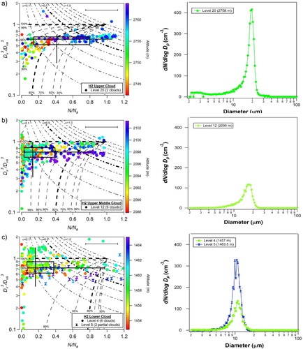
We first examine whether the cloud response to entrainment mixing depends on the (normalised) vertical location within the cloud. We look at how mixing type changes as a function of altitude by comparing mixing diagrams for the various cloud quartile regions: lower, lower middle, upper middle, and upper (refer to Fig. 1 for relative altitude ranges of the cloud regions). In the following plots, the mixing diagrams are produced including all clouds sampled with widths greater than ~300 m within each quartile region. Each data point represents a ~10 m averaged in-cloud measurement. There is no distinction between individual clouds, only sampling levels. We show mixing diagrams separated by altitude for two different flights, L2 and H2 (chosen because more in-cloud data is available on these days) in Figs. 5 and 6. The box-and-whiskers show the values for the 5, 25, 50 (i.e. median), 75 and 95 percentiles for both axes.

Fig. 5 1-Hz data plotted as a function of altitude and corresponding average DSD for each level (coloured markers and lines based on altitude) for (a) upper cloud, (b) lower-middle cloud and (c) lower cloud with 2-D box and whiskers representing 95, 75, median, 25 and 5 percentiles of all levels.

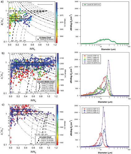
Fig. 6 1-Hz data plotted as a function of altitude (coloured markers) and corresponding average DSD for each level and individual clouds (coloured lines based on altitude) for (a) upper cloud, (b) upper-middle cloud and (c) lower cloud with 2-D box and whiskers representing 95, 75, median, 25 and 5 percentiles of all levels.

One common feature of all the mixing diagrams we show, regardless of altitude, is that there is much more variability in N/N_a as compared with . Based on the 25 and 75 percentile values, the scatter in exhibits a variability of±20 to 30%. On the other hand, N/N_a exhibits a variability of ± a factor of 2 to 4 (i.e.±200 to 400%). There is no obvious trend in this variability (i.e. the aspect ratio of the 25 to 75 percentile box) with altitude. These data show that liquid water variability at all altitudes is driven primarily by variability in drop concentration rather than drop size. Using the 5 and 95 percentile values leads to the same qualitative conclusion, although the discrepancy is not quite as large. This demonstrates that for these non-precipitating clouds whose loss of liquid water comes primarily from entrainment and evaporation, the predominant cloud response appears inhomogeneous at the averaging of length scales of these observations (~10 m).

We next look to see how mixing can change with altitude by first using L2 as a case study. In the lowest part of the cloud (Fig. 5c), data clusters around the inhomogeneous mixing line =1, with the median value of ~ 1.2. A reasonable explanation for this ratio being greater than unity is that our assumed cloud base was slightly wrong, since adiabatic drop size is extremely sensitive to height above cloud base in the lower cloud region. Adiabatic calculations show this is the equivalent of a bias in cloud base of ~0 to 20 m, which is not a surprising amount. Note that this bias does not affect the discussion here, since we are looking at relative shifts of the data, which all use the same assumed cloud base. Comparing the different cloud regions in Fig. 5, we see that shifts from ~1.2 in the lower cloud to values of ~0.8 and 0.6 in the lower-middle and upper cloud regions, respectively. These changes are consistent with a shift in the cloud response to entrainment mixing from more inhomogeneous in the lower regions of these Cu to more homogeneous at the upper regions.

In order to test if differences in between regions are statistically significant, the Wilcoxon rank-sum test was used as described in section 3 (refer to Table 2). For this case (L2), we see that four of the comparisons (e.g. lower vs. upper middle) of the populations reveal a statistically significant (p=0.01) decrease with height. No statistically significant cases where increases with height are seen for the comparisons on this day.

We now examine all four days together by comparing results from different altitudes for each day. Cases L1 and H1 have reduced sample sizes at lower altitudes and so statistically significant comparisons cannot be made on these days and thus are not included in Tables 2 and 3. The results from all days combined show that changes with height to a statistically significant degree in seven comparisons, of which six indicate a decrease with altitude and one case with the converse. Looking at all cases, regardless of statistical significance, 13 of 16 comparisons indicate a decrease in with altitude, while three show an increase. We interpret the patterns in these data as strongly supporting the hypothesis that mixing becomes more homogeneous with altitude in non-precipitating cumulus. Past researchers have also found evidence of both homogeneous and inhomogeneous mixing acting in concert (Jensen and Baker, 1989; Paluch and Baumgardner, 1989).

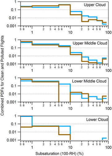
We use a different analysis of these data to illustrate the shift in mixing with altitude. Probability distribution functions (PDFs) were calculated based on the number of samples that fall between categories of entrained air relative humidity. In other words, referring back to Fig. 4, we determine the fraction of samples that lie between the dashed lines representing the homogeneous mixing of air with RH between 80 and 90%, 90 and 95%, etc. This allows for an analysis of the proportion of data which lies within different relative humidity mixing categories. RH bins for this PDF analysis are from 100–99% (which we interpret as inhomogeneous mixing), 99–95%, 95–90%, 90–80%, 80–70%, 70–50% and 50–30%. Note that Fig. 7 is plotted with the y-axis as sub-saturation for clarity at high RH, so 80–90% RH is plotted as 10–20% sub-saturation. Data with N/N_a or values greater than 1.2 or less than 0.1 were excluded. A parcel of air whose drops have experienced a mixture of homogeneous and inhomogeneous mixing will appear on the mixing diagram as having experienced one single homogeneous mixing event, but at a higher RH than was actually encountered. One can see this by following a line of constant adiabaticity in the sample mixing diagram in Fig. 4. The PDFs in Fig. 7 show that as height above cloud base increases, the number of samples that plot in lower relative humidity ‘wedges’ increases. This is evident in both the lower and the higher pollution examples. This different approach to analysing the data further supports the hypothesis that homogeneous mixing becomes more important at higher levels in a cloud.

Fig. 7 PDF of relative humidity mixing wedges. Vertical profiles of turbulence quantities for individual flights. Combined histograms for lower pollution flights, L1 and L2 (blue curves), and higher pollution flights, H1 and H2 (brown curves). Data are first binned by relative humidity according to RH curves presented on mixing diagrams, with bins defined for RH 10–30%, 30–50%, 50–70%, 70–80%, 80–90% 90–95%, 95–99% and 99–100% (although the upper limit is plotted as 99.5%). The 99–100% humidity range would contain parcels that experienced perfect inhomogeneous mixing. The bins are then weighted to accommodate the differences in bin widths. Finally, sub-saturation is calculated for each bin by taking 100-RH for each of the bin boundaries. Such that a RH bin for 99–95% has a sub-saturation of 1–5%. This allows us to look at the 99–90% humidity range in more detail. Number counts for 10–30% bin represent data with N/N_a values less than 1.2 or values less than 0.1. Data with greater than 1 are not shown.

Looking at variations in N/N_a there is no statistically significant difference when comparing vertical cloud regions and no observed trend in N/N_a with increased altitude, which is consistent with inspection of Figs. 5 and 6.

It must be noted that the points on the mixing diagrams for the chosen layers often do not appear to fall ‘perfectly’ along the homogeneous mixing lines and there is much scatter. This is due in part to the large number of samples and different clouds at each level. Another consideration is that aircraft observations provide only instantaneous observations and it is not possible to know the mixing history of any given sample.

4.1.1. Adiabaticity profiles

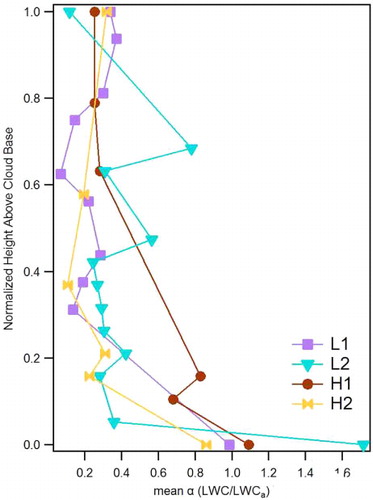
Adiabaticity α can also be compared among different cloud altitude regions. Table 2 shows that of the 16 available comparisons, only three are statistically significant, with two of the three supporting an increase in α with height. Nine of 16 comparisons indicate an increase in α with cloud height, and the other seven indicate a decrease. These data thus support a null-hypothesis adiabaticity profile where there's no clear change with altitude. To support this point, vertical profiles of α are plotted in Fig. 8 following Fig. 4c of Wood (2005). Aside from points in the bottom-most 10 to 20% of each cloud, there is no clear trend in adiabaticity with height. This is contrary to stratocumulus, where observations show adiabaticity decreasing with height, most strongly in the region near cloud top where entrainment occurs. Wood (2005) also reported profiles for boundary layer clouds under well mixed conditions that resemble profiles of α shown here.

Fig. 8 Vertical profiles of α. Vertical profiles of adiabaticity α=LWC/LWC_a for L1, L2, H1, and H2 as a function of normalised height above cloud base.

4.1.2. Role of secondary activation

For each mixing diagram, average droplet size distributions (DSDs) are presented for each level for cases L2 and H2 (Figs. 5 and 6, respectively). In the case of H2, we also present individual cloud DSDs due to the limited number of levels sampled during the flight as compared to L2. For both L2 and H2, we see that the size distribution generally shifts to larger median diameters as altitude increases, as expected, with the narrowest distributions observed near cloud base. For H2 we see no bimodal size distributions, nor any ‘shoulder’ at smaller drop sizes, and thus no evidence that secondary activation is a significant process in these clouds. For L2, we see some broadening to smaller diameters at two levels (levels 6 and 10), as well as one bimodal distribution (level 8). Regarding the latter, an analysis of the 1 Hz DSDs for this level reveals two distinct, mono-modal DSDs separated in time, that is, from two different cloud populations. Thus, this is not a signature of secondary activation. For levels 6 and 10, the broadening to smaller sizes does not appear to be consistent with model predictions of DSDs substantially impacted by secondary activation (e.g. Erlick et al., 2005; Lasher-Trapp et al., 2005), although we cannot entirely rule this out. That we see little evidence of secondary activation is not greatly surprising as the drop concentrations in these clouds is generally very high (many hundred per cm³) which implies a large total drop surface area and therefore a very strong condensational sink. In order to generate substantial supersaturations under these conditions (even for diluted parcels), very large upward velocities are needed but unlikely to be commonplace due to the shallow nature of these cumuli. Thus, theory would predict that such clouds are not strongly impacted by secondary activation and DSDs are consistent with this prediction. The data shows that while there is some possibility that secondary activation has impacted a small fraction of our observations, the large majority of our data shows no evidence of such effects. Therefore, secondary activation does not appear to substantially impact our mixing diagram observations or our inferences drawn from them.

4.1.3. Interpretation of vertical structure

What might be the physical mechanism causing the observed shift towards a greater degree of homogeneous mixing with altitude? We return to eq. (4) which shows that changes in ɛ and/or D can change the Damköhler number, Da, and hence the nature of mixing. Since D generally increases with height in non-precipitating clouds (cf. size distributions in Figs. 5 and 6), Da will tend to decrease with altitude; thus, mixing is predicted to appear more homogeneous as altitude increases. More quantitatively, we find that D increases by a factor of ~2 to 3 from cloud base to cloud top; this leads to a decrease in Da of a factor of ~4 to 10.

Furthermore, our observations are consistent with an increase in turbulence with altitude. Figure 9 shows vertical profiles of two turbulence measures and , where ω is the vertical velocity (m/s) and θ is the potential temperature (K). Both measures are calculated similarly as show below,7 8

Fig. 9 Vertical profiles of turbulence quantities for individual flights. Vertical profiles of (a) fluctuations in vertical velocity, and (b) fluctuations of potential temperature, . Means across all four flights (L1, L2, H1 and H2) are calculated and one standard deviation is shown in grey for each normalised altitude bin.

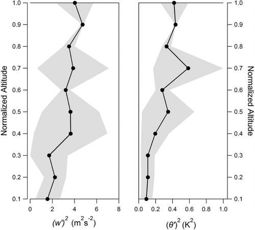
where ω_i and θ_i are instantaneous values in non-precipitation cloud samples>300 m in length obtained by the sorting methods as described above for other in-cloud data. and are calculated based on the mean of all data, whether 1 Hz (for full cloud passes) or 5 Hz values (for cloud edge-centre sampling) for each flight.

Both measures show some increase with normalised cloud height when all days are composited. We have composited all days in order to best reveal this overall trend; inspection of the individual days shows that this trend is not driven by observations from any single day. The apparent increase in turbulence with altitude can be used to estimate the increase in ɛ with altitude. From eq. (4), this also causes Da to decrease with height, thereby shifting mixing more towards the homogeneous end-member. We crudely estimate from Fig. 9 that the increase in to be a factor of ~2 (from 2 to 4 m²s⁻²). Turbulence scaling theory predicts ɛ to scale as , so the increase in ɛ from the lowest to highest cloud regions is a factor of ~3, which is the same order of magnitude as the change in D. Taken together, and assuming that l is constant (the validity of which is unclear), the overall change in Da is therefore a factor of ~10 to 30. Theory [eq. (4)] would predict that our observed trends in ɛ and D with altitude should lead to a cloud response to entrainment mixing that appears more homogeneous as altitude increases. Taken as a whole, our observations strongly support this prediction.

4.2. Mixing at cloud edges vs. centre

We now turn our attention to how mixing type changes as a function of horizontal location in cloud. Using high rate 5 Hz (~10 m) data, we compare cloud edges and centres. ‘Cloud edge’ data was obtained by selecting the first 1-s of data upon entry into cloud and the last 1-s of data prior to exiting cloud, for a total of 10 samples per cloud. Cloud centre data was obtained by selecting the middle 2-s of each cloud pass, for a total of 10 centre samples per cloud. Each level contains samples from a different number of clouds dependent on the flight path and cloud targets chosen by the pilots. Given a mean cloud size of ~700 m, the edges represent on average the outer ~15% of the cloud radius (i.e. 50 out of 350 m), though this percentage varies due to the wide range in cloud sizes.

In all cases, the most noteworthy difference between edges and centres is the shift in N/N_a (Table 3), while values are not statistically different between these two populations at any altitude for any of our flights days. This is illustrated in Fig. 10a and b, where two examples, one from L2 and one from H1, are shown. For the 13 levels with substantial data across the four days, the mean ratio of N/N_a for centres compared to edges is 2.2 (range 1.7 to 3.8), excluding the one level that exhibited a higher value of N/N_a at cloud edge compared to centre (lower middle on H2). Of the 13 levels, seven of the differences are significant with p<0.01, and three more levels would be statistically significant at p<0.05 (see Table 3 for full Wilcoxon signed-rank-sum test results).

Fig. 10 Mixing diagrams displaying edge and centre data. Five-hertz cloud edge and centre samples for (a) the lower-middle region for L2, and (b) the upper region of H1. Edges for all levels are red circles, centres for all levels are blue squares with 2-D box and whiskers representing 95, 75, median, 25 and 5 percentiles of all levels.

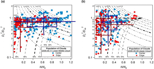
Table 3. Full flight Wilcoxon ranked-sum test results for α weighted N/N_a values for cloud centres and edges. Cloud edges and cloud centres for each cloud region are compared using the Wilcoxon signed-rank-sum test. Comparisons that result in statistically significant values, with p<0.01 are boldfaced

	Edge Mean±σ N/Na	Centre Mean±σ N/Na	p
L1 (2006-Aug-26)
Lower Middle	0.23±0.25	0.41±0.29	0.0386
Upper Middle	0.12±0.13	0.28±0.22	0.0386
Upper	0.23±0.14	0.45±0.15	0.1492
H1 (2006-Sept-08)
Upper Middle	0.14±0.23	0.30±0.29	0.0010
Upper	0.21±0.24	0.31±0.18	0.0420
L2 (2006-Sept-11)
Lower	0.15±0.19	0.47±0.28	0.5202
Lower Middle	0.26±0.31	0.62±0.42	0.0078
Upper Middle	1.17±1.03	4.42±1.37	0.0001
Upper	0.06±0.07	0.15±0.14	0.0001
H2 (2006-Sept-15)
Lower	0.18±0.25	0.30±0.26	0.1305
Lower Middle	0.29±0.32	0.19±0.26	0.0009
Upper Middle	0.13±0.18	0.36±0.32	0.0010
Upper	0.26±0.24	0.66±0.35	0.0001

Interestingly, there is little change in when comparing edges to centres; that is, the mean volume diameter of drops found at cloud edge is almost the same as in the middle of the cloud at the same altitude for all 13 cases (illustrated in Fig. 10). The difference in liquid water between cloud centres and edges at each altitude is expressed almost entirely as a change in N/N_a. Put another way, air parcels at cloud edge have lower LWCs than those at cloud centres, and this occurs as a result of lower drop concentrations and not because of a decrease in drop size. Note that because decreases with altitude as discussed above, the value of that is consistent between cloud centre and edge decreases with altitude.

If cloud edges were simply like cloud centres but with a greater degree of dilution, then we should see, at least at upper cloud levels, some degree of homogeneous mixing, which would simultaneously decrease and N/N_a. Since no statistically significant changes in are observed between centres and edges, this supports the idea that the mixing causing cloud edge dilution is different from the mixing that dilutes the whole cloud at that altitude. 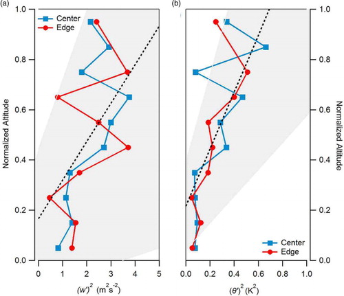Figure 11 shows centre and edge observations of and as a function of altitude with both increasing with normalised cloud height when all days are composited. There is no consistent trend or difference between edge and centre measurements of and . Thus, differences in turbulence intensity do not appear to explain the differences between cloud centre and edge. These observations may be explained if edges are biased towards mixing by smaller eddies while larger eddies are able to penetrate deeper into cloud. This would result in short mixing time scales and more inhomogeneous type mixing at the edges relative to centres [eq. (3)]. However, in order to test this theory a detailed analysis of turbulent properties at cloud edge would be required and such data are not currently available.

Fig. 11 Vertical profiles for centres and edges. Data for (a) fluctuations in vertical velocity, and (b) fluctuations of potential temperature, . Blue curves with square markers represent data from cloud centres for L1, L2, H1 and H2. Red curves with circle markers represent data from cloud edges for L1, L2, H1 and H2. Linear regressions for composites of all days, including both centre and edges (black dashed lines) and 95% confidence intervals for slopes are also represented (shaded area) showing the increase in turbulent quantities with height.

We speculate here that the simplest explanation for this observation is that cloud edge air originates from the middle of the cloud, and subsequently moves towards the edge, entrains sub-saturated air, and responds inhomogeneously. This could occur if air at cloud centres tends to remain close to its neutral buoyancy altitude despite turbulent mixing that might cause that air to move to a different altitude. If that air stays at the level long enough, then it can experience lateral entrainment and thus cloud edge and cloud centre air can be related. This mechanism also requires that the buoyancy of the cloud edge air not change by very much after entrainment occurs so that these parcels remain at a similar altitude. Note that if air with a given value of moves vertically and adiabatically, this ratio will tend to increase with upward motion and decrease with downward motion. The fact that, in the previous section, we find the trend in to be opposite this tendency suggests that vertical transport of cloud edge parcels is a less satisfactory explanation for the observed differences between edges and centres. More data would be needed to demonstrate whether this mechanism is indeed valid and we leave further exploration of this topic for future study.

Wang et al. (2009) also used aircraft observations to examine the horizontal structure of clouds. Although their data is not represented in mixing diagram form, their observations tend to show that, relative to cloud centres at the same altitude, cloud edges exhibit both lower N and D_v (cf. their Fig. 6). Since D_v decreases, their observations suggest that cloud edges are not simply inhomogeneously diluted cloud centres. One potential explanation for the discrepancy between these studies is that the Damköhler number is different between the studied clouds (which include continental Cu over Wyoming and Arizona, and trade Cu over the Atlantic from the RICO project). Smaller Da shifts mixing towards the homogeneous end-member and could result from increases in environmental RH, energy dissipation rate or cloud LWC, or decreases in cloud drop size. Whether these factors account for the differences between these studies cannot be determined here. Our results are broadly consistent with those presented in Lehmann et al. (2009), in which homogeneous mixing occurs near cloud cores and inhomogeneous mixing occurs in more dilute cloud regions (i.e. edges).

4.3. Effect of aerosols

Aerosol concentration plays a role in determining the size of cloud drops, in turn potentially affecting both time scales τ_evap and τ_phase. Here we investigate the dependence of mixing on aerosol concentration by comparing cloud regions, lower, middle and upper levels in the statistically sampled clouds. It is important to recognise that the clouds were of different thicknesses and that cloud base varied from day-to-day and during each flight. Thus comparisons are made between regions rather than by absolute altitude. Typical clean background aerosol concentrations were not observed during the GoMACCS project. Our two highly polluted cases, H1 and H2, have accumulation-mode aerosol concentrations N_acc of ~1600 and 900 cm⁻³, respectively. Our two lower pollution cases, L1 and L2, have mean N_acc of 400 and 600 cm⁻³, respectively. Thus, N_acc differs among these cases by between a factor of ~1.5 and 4. Mean cloud drop concentrations on the four days are shown in Table 1. While the aerosol conditions are substantially different, the drop concentrations are less so, which is consistent with the negative feedback between cloud condensation nuclei (CCN) concentration and supersaturation; that is, higher CCN concentrations tend to suppress water supersaturation, leading to a smaller fraction of CCN being activated (Feingold and Siebert, 2009).

It is possible that aerosol can change the cloud response to entrained air because the change in drop size D changes Da. Do we see any evidence of this effect? Figure 7 shows that the higher pollution flights have slightly narrower PDFs and, hence, leans slightly more towards inhomogeneous mixing, than lower pollution flights for low and mid-cloud levels. This small difference disappears at cloud top. The sense of this shift is what we expect based on eq. (4), as decreasing D should promote a shift to more inhomogeneous mixing. However, the differences are not statistically significant. One potential reason for this is the difference in drop size between clean and polluted cases is at most a factor of 2, which causes a change in Da of at most a factor of 4. This is considerably smaller than the factor of 10 to 30 by which Da changes between cloud top and bottom, suggesting that any effect would be much more subtle compared with the shift towards homogeneous mixing with altitude. Thus, we tentatively conclude that our data are weakly consistent with aerosol-induced shifts in mixing, but more data, and probably at lower aerosol concentrations, would be necessary to establish such a mechanism with statistical certainty.

5. Conclusions

This paper examines entrainment mixing during four research flights which sampled non-precipitating continental cumulus for different aerosol concentrations during the GoMACCS campaign. We address three main questions: (1) How does entrainment mixing affect cloud drop size distributions? (2) What does this mixing depend on? and (3) Can aerosol influence the effects of entrainment mixing? Our main findings are:

1. Variability in LWC is predominantly governed by variability in cloud drop concentration, with the contribution of cloud drop size variability being an order of magnitude lower. Hence, entrainment mixing in these cumulus clouds appears primarily inhomogeneous.

2. The net cloud response to entrainment mixing shifts towards more homogeneous in nature with increasing altitude. This is consistent with increases in the Damköhler number by a factor of ~10 to 30 between cloud base and top, which results from increases in cloud drop size and turbulent kinetic energy with altitude.

3. Cloud edges are more dilute than cloud centres at the same altitude, and this dilution occurs inhomogeneously (at constant drop size). This difference is maintained at all altitudes, even as homogeneous mixing becomes on average more prominent with altitude. This observation does not appear to be due to differences in turbulent kinetic energy.

4. Our data are weakly consistent with the prediction that polluted clouds may respond to entrainment mixing more inhomogeneously than cleaner clouds, but this was not established with a reasonable degree of statistical certainty.

We emphasise that this study examines the net effect, or imprint, of entrainment on cloud microphysical properties that are observed at instantaneous moments. The actual process of entrainment mixing is almost certainly highly variable within every cloud and what we observe here is merely the mean behaviour averaged over time and space.

6. Appendix

A.1. Nomenclature

Table

α	LWC dilution ratio
ɛ	Energy dissipation rate
ρa	Air density (kg/m^3)
ρw	Density of water (kg/m^3)
τevap	Time scale for evaporation of a cloud drop
τphase	Time scale for re-establishing saturation after entrainment
τmix	Time scale for entrainment mixing
θ	Potential temperature (K)
	Potential temperature fluctuation
k	Constant, 4x10^−10m^2s^−1
l	Mixing length scale
qT	Total water mixing ratio (g/kg)
qTa	Adiabatic total water mixing ratio (g/kg)
ql	Liquid water mixing ratio (g/kg)
qla	Adiabatic liquid water mixing ratio (g/kg)
	Vertical velocity (m/s)
	Vertical velocity fluctuation
CDNC	Cloud drop number concentration
D	Drop diameter (µm)
Da	Damköhler number
Dv	Observed mean volume diameter (µm^3)
Dva	Adiabatic mean volume diameter (µm^3)
DSDs	Drop size distributions
LWC	Liquid water content
LWCa	Adiabatic liquid water content
N	Cloud drop number concentration (cm^−3)
Na	Adiabatic cloud drop number concentration (cm^−3)
Nacc	Leg mean accumulation-mode aerosol concentration (cm^−3)
Ntot	Total aerosol concentration (cm^−3)
P	Pressure (mb or Pa)
RH	Relative humidity (%)
T	Temperature (C or K)
Td	Dew point temperature (C or K)

References

- Baker M , Corbin F , Latham J . The influence of entrainment on the evolution of cloud droplet spectra 1. A model of inhomogeneous mixing. Quart. J. R. Met. Soc. 1980; 106: 581–598.
- Baker M. B , Breidenthal R. E , Choularton T. W , Latham J . The effects of turbulent mixing in clouds. J. Atmos. Sci. 1984; 41: 299–304.
- Baumgardner D , Jonsson H , Dawson W , O'Connor D , Newton R . . The cloud, aerosol and precipitation spectrometer: a new instrument for cloud investigations. Atmos. Res. 2001; 59, 60: 251–264.
- Bewley J. L , Lasher-Trapp S . Progress on predicting the breadth of droplet size distributions observed in small cumuli. J. Atmos. Sci. 2011; 68: 2921–2929.
- Burnet F , Brenguier J.-L . Observational study of the entrainment-mixing process in warm convective clouds. J. Atmos. Sci. 2007; 64: 1995–2011.
- Chuang P , Saw E , Small J , Shaw R , Sipperley C , co-authors . Airborne phase doppler interferometry for cloud microphysical measurements. Aerosol Sci. and Tech. 2008; 42: 685–703.
- Derkson J. W. B , Roelofs G.-J. H , Rockmann T . Influence of entrainment of CCN on microphysical properties of warm cumulus. Atmos. Chem. Phys. 2009; 9: 6005–6015.
- Erlick C , Khain A , Pinsky T , Segal Y . The effect of wind velocity fluctuations on drop spectrum broadening in stratocumulus clouds. Atmos. Res. 2005; 75: 15–45.
- Feingold G , Siebert H . Cloud-aerosol interactions from the micro to the cloud scale. Clouds in the Perturbed Climate System: Their Relationship to Energy Balance, Atmospheric Dynamics, and Precipitation. 2009; 319–338. Vol. 2, The MIT press, Cambridge, MA.
- Friehe C. A , Khelif D . Fast-response aircraft temperature. J. Atmos. Ocean. Tech. 1992; 9: 784–795.
- Hill T , Choularton T . An airborne study of the microphysical structure of cumulus clouds. Quart. J. R. Met. Soc. 1985; 111: 517–544.
- Jensen, J. and Baker, M. 1989. A simple model of droplet spectral evolution during turbulent mixing. J. Atmos. Sci. 46, 2812–2829..
- Jensen J. B , Austin P. H , Baker M. B , Blyth A. M . Turbulent mixing, spectral evolution and dynamics in a warm cumulus cloud. J. Atmos. Sci. 1985; 42: 173–192.
- Jiang H , Xue H , Teller A , Feingold G , Levin Z . Aerosol effects on the lifetime of shallow cumulus. Geophys. Res. Lett. 2006; 33: L14806.
- Korolev A. V , Isaac G. A . Drop growth due to high supersaturation caused by isobaric mixing. J. Atmos. Sci. 2000; 57: 1675–1685.
- Lasher-Trapp S. G , Cooper W. A , Blyth A. M . Broadening of droplet size distributions from entrainment and mixing in a cumulus cloud. Quart. J. R. Met. Soc. 2005; 131: 195–220.
- Latham J , Reed R. L . Laboratory studies of effects of mixing on evolution of cloud droplet spectra. Quart. J. R. Met. Soc. 1977; 103: 297–306.
- Lehmann K , Siebert H , Shaw R. A . Homogeneous and inhomogeneous mixing in cumulus clouds: dependence on local turbulence structure. J. Atmos. Sci. 2009; 66: 3641–3659.
- Lu M , Jonsson H , Chuang P , Feingold G , Flagan R , co-authors . Aerosol-cloud relationships in continental shallow cumulus. J. Geophys. Res. 2008; 113 D15201.
- Paluch I. R , Baumgardner D. G . Entrainment and fine-scale mixing in a continental convective cloud. J. Atmos. Sci. 1989; 46: 261–280.
- Small J. D , Chuang P. Y , Feingold G , Jiang H . Can aerosol decrease cloud lifetime?. Geophys. Res. Lett. 2009; 36: L16806.
- Su C.-W , Krueger S. K , McMurty P. A , Austin P. H . Linear eddy modeling of droplet spectral evolution during entrainment and mixing in cumulus clouds. Atmos. Res. 1998; 41–58. 47, 48 .
- Telford J. W , Keck T. S , Chai S. K . Entrainment at cloud tops and the droplet spectra. J. Atmos. Sci. 1984; 41: 3170–3179.
- Wang Y , Geerts B , French J . Dynamics of the cumulus cloud margin: an observational study. J. Atmos. Sci. 2009; 66: 3660–3677.
- Wood R . Drizzle in stratiform boundary layer clouds: part I: vertical and horizontal structure. J. Atmos. Sci. 2005; 62: 3011–3033.