A whole-air relaxed eddy accumulation measurement system for sampling vertical vapour exchange of elemental mercury

Abstract

An apparatus relying on relaxed eddy accumulation (REA) methodology has been designed and developed for continuous-field measurements of vertical Hg⁰ fluxes over cropland ecosystems. This micro-meteorological technique requires sampling of turbulent eddies into up- and downdraught channels at a constant flow rate and accurate timing, based on a threshold involving the sign of vertical wind component (w). The fully automated system is of a whole-air type drawing air at a high velocity to the REA sampling apparatus and allowing for the rejection of samples associated with w-fluctuations around zero. Conditional sampling was executed at 10-Hz resolution on a sub-stream by two fast-response three-way solenoid switching valves connected in parallel to a zero Hg⁰ air supply through their normally open ports. To suppress flow transients resulting from switching, pressure differentials across the two upstream ports of the conditional valves were minimised using a control unit. The Hg⁰ concentrations of the up- and downdraught channel were sequentially (each by two consecutive 5-minute gas samples) determined after enhancement collection onto gold traps by an automated cold vapour atomic fluorescence spectrophotometer (CVAFS) instrument. A protocol of regular reference sampling periods was implemented during field campaigns to continuously adjust for bias that may exist between the two conditional sampling channels. Using a 5-minute running average was conditional threshold, nearly-constant relaxation coefficients (β_s) of ~0.56 were determined during two bi-weekly field deployments when turbulence statistics were assured for good quality, in accordance with previously reported estimates. The fully developed REA-CVAFS system underwent Hg⁰ flux field trial runs at a winter wheat cropland located in the North China Plain. Over a 15-d period during early May 2012, dynamic, often bi-directional, fluxes were observed during the course of a day with a tendency of emission (Hg⁰ median flux of 77.1 ng m⁻² h⁻¹) during daytime and fluctuation around zero (Hg⁰ median flux of 9.8 ng m⁻² h⁻¹) during nighttime.

• air-surface gas exchange
• elemental mercury
• micro-meteorological technique
• cropland ecosystem flux

To access the supplementary material to this article, please see Supplementary files under Article Tools online.

1. Introduction

In the unperturbed lower troposphere, Hg⁰ (representing >95% of total mercury) has a turnover time of up to 1 yr and thus undergoes transport on hemispherical scales. Eventually deposited to ground and water surfaces primarily as oxidised Hg (Hg^II species in the gas phase, acronym GOM or attached to aerosols), it may undergo reduction by biochemical and photolytic processes and regained as Hg⁰ may be re-emitted to the atmosphere. Since pre-industrial times, anthropogenic activities have significantly increased the global atmospheric mercury actively cycling between the atmosphere, land and oceans (Lindberg et al., 2007; Selin et al., 2008). Together, emissions of natural and previously deposited mercury from marine and terrestrial surfaces (predominantly as Hg⁰) are associated with large uncertainties comparable to annual anthropogenic emissions (a mixture of Hg⁰, gas-phase Hg^II and Hg attached to aerosols) in magnitude (Pirrone et al., 2009; Sommar et al., 2013).

The cycling of Hg through terrestrial ecosystems includes a complex and not fully understood process via soil and vegetation pools in which Hg has significantly different residence times (Obrist, 2007; Smith-Downey et al., 2010). Atmosphere–phytosphere interaction plays an important role here as the majority of Hg in aerial parts of terrestrial plants is obtained from air (Grigal, 2003). In contrast to wet deposition, gas transfer processes of sparingly soluble Hg⁰ are dynamic and largely bi-directional (i.e. potentially include emission as well as dry deposition events) over a typical day (Lindberg et al., 1998). Similar to NH₃ (Sutton et al., 1995), ambient air Hg⁰ concentration-dependent net exchange over plants exhibits growing seasonal trends as well as plant-specific patterns among others (Graydon et al., 2006; Poissant et al., 2008; Bash and Miller, 2009). As discussed in Mason (2009), many studies to constrain air-terrestrial ecosystem Hg⁰ gas exchange suffer from limited temporal and spatial scale, or from using indirect approaches associated with aggravating artefacts. To gain a better understanding, it is important to determine spatial and temporal variability in the air-natural surface exchange of Hg⁰ as it relates to environmental, physicochemical, meteorological factors and surface characteristics. The interactions among these factors potentially lead to highly variable Hg⁰ flux, making it imperative to perform experimental studies with an adequate technique over a sufficiently long time scale to pinpoint crucial regulating mechanisms and seasonal patterns.

East Asia has emerged as the world's largest source region of atmospheric mercury mainly due to a rapid expansion in fossil fuel combustion and increased industrialisation in contrast to significant reduction in anthropogenic emissions in Europe and North America. Because of the elevated deposition in the region, the relative importance of re-emissions from impacted terrestrial ecosystems is potentially large (Streets et al., 2005). Concerning modelling studies of the natural Hg emissions from China, there exists a large discrepancy not only for the magnitude of total emissions but also concerning the relative importance of biogenic sources (Quan et al., 2008; Shetty et al., 2008).

In this region, field observations of Hg⁰ air-surface exchange in terrestrial settings are comparatively scarce and largely confined to non-vegetated surfaces (Ci et al., 2012; Fu et al., 2012a). Up until now in China, solely flow-through dynamic flux chambers (DFCs) covering a small plot of ≤0.1 m² have been employed for such studies (e.g. Feng et al., 2004, 2005; Wang et al., 2005, 2006, 2007a, 2007b; Fu et al., 2008, 2012a, 2012b; Zhu et al., 2011; Zhu et al., 2013). Enclosure methods are of relatively low cost, easy to operate and straightforward. However, small DFCs may only be applied to bare soil, water or surfaces with very low vegetation. They also suffer from disadvantages, including unavoidable influence on the microclimate over the plot studies and isolation from outside air. Moreover, DFCs employed in the aforementioned studies lack the appropriate design to achieving an uniform flow field over the surface substrate investigated, and thus are not able to standardise its internal shear stress properties and make scaling with atmospheric surface layer conditions feasible (Lin et al., 2012).

For the study of the Hg⁰ surface exchange process over an ecosystem scale (e.g. an agricultural crop field or a forest canopy), micro-meteorological (MM) techniques represent an attractive alternative to enclosure techniques. They allow spatially averaged measurements over a large area without disturbing ambient conditions and may serve as independent tests of process-based models but are in turn technically more demanding and require detailed knowledge of the prevailing MM conditions and the source area. An extensive review of the application of different MM methods to measure air-natural surface mercury flux can be found elsewhere (Sommar et al., 2013), which may useful to compare present work with previous ones. Briefly, most MM methods [modified Bowen-ratio (MBR), aerodynamic (AER) and relaxed eddy accumulation (REA) method] are apt to be applied to mercury flux measurements (currently with the exception to the eddy-covariance (EC) given the lack of a fast-response ambient air Hg⁰ sensor). Nevertheless, the coupling with commercially available analytical instrumentation for measuring ambient air Hg potentially renders continuous and unattended MM flux measurements possible to be accomplished (Gustin et al., 1999; Edwards et al., 2005). In Korea, Kim et al. have performed AER measurements of Hg⁰ flux over paddy fields (Kim et al., 2002, 2003), landfills (Kim et al., 2001; Nguyen et al., 2008) and residential settings (Kim and Kim, 1999). These studies were of relative short duration (weekly to bi-weekly) and not seasonally resolved by repeated measurements. Given the paucity of broad seasonal Hg⁰ flux datasets collected over terrestrial landscapes in East Asia, there is a strong incitement to develop a reliable and robust MM system to be deployed for such studies.

REA is a conditional sampling technique derived from EC, which has been proposed by Hicks and McMillen (1984) and developed by Businger and Oncley (1990) as a relaxation of the eddy accumulation (EA) approach suggested by Desjardins et al. (1984). As in EC, REA measurements are performed at a single point above the surface, but here is the fast-response gas sensor required in EC substituted by fast-response switching valves, which enables the separation of up- and down-draughts present in the air column due to turbulent eddies into conditional sampling reservoirs. Each MM method has distinct advantages and disadvantages. However, those based on the concept of turbulent diffusion (MBR, AER) require measurements of gradients, which become very small close to vegetation canopies (Moncrieff et al., 1997). Although REA involves comparatively sophisticated equipment, it is plausibly the most suitable of the techniques for biogenic Hg⁰ flux studies (Cobos et al., 2002; Bash, 2006).

The objective of this research is to develop a REA system as a prototype for measurement of Hg⁰ exchange in representative terrestrial ecosystems (e.g. agricultural crop fields) of China. As recently emphasised in a feature paper by Ci et al. (2012), there is a need to integrate Hg flux measurements in China into a nationwide or regional network, such has been accomplished for net ecosystem CO₂ exchange in ChinaFLUX for a decade and to implement MM techniques as a resource for its exploration. This work was conducted in parallel with implementing a novel type of DFC to gauge Hg⁰ fluxes over defined surfaces (e.g. soil plots included in a crop field) within the biomes investigated (Lin et al., 2012). In the present contribution, we introduce the configuration of our REA system and describe the coupling to a cold vapour atomic fluorescence spectrophotometer (CVAFS) and describe the procedures for measurement of Hg⁰ fluxes based on investigations with respect to theoretical, methodological, environmental and instrumental requirements and limitations. Finally, measurement results of Hg⁰ flux obtained from the developed REA system deployed for a bi-weekly period at a winter wheat cropland are briefly discussed. Nomenclature and symbols used in the following sections are generally explained in the running text. Nevertheless, as an aid to the reader, frequently utilized symbols are as well tabulated in an appendix.

2. Materials and methods

2.1. Site description

Research was performed at Longli Grassland Reserve (LGR, 26°21′N, 106°54 ′E, 1635 m a.s.l.) and at Yucheng Comprehensive Experimental Station (YCES, 36°57′N, 116°36′E, 19 m a.s.l.). The later facility belongs to Chinese Academy of Sciences (CAS). A map showing the location of the sites is shown in the supplementary material (Fig. S1). LGR is located in Guizhou Province, SW China. The site consists of a relatively flat, grazed, highland prairie landscape (level differences<±4 m within method fetch). The field testing of the REA system was performed at LGR. The fieldwork was of bi-weekly duration in July 2011.

More comprehensive field testing and initial flux monitoring trials was conducted at the experimental farm of YCES. It is located in a semi-rural area of Shandong province on the North China Plain circa 350 km south of Beijing. The farmland is continuously cropped with winter wheat (October–June) and summer maize (July–September) in rotation during the year and within a radius of ~5 km surrounded by unbroken farmlands with identical crop at the similar growth stage. The upper texture of soil is a silty loam with a substantial degree of alkalinity and salinity. Surface soils are relatively meagre in organic matter (≤20 g kg⁻¹) but nevertheless slightly enriched in heavy metals (e.g. Cu, As, Hg and Cd). Concerning Hg, by exhibiting a high bioconcentration factor, wheat grain samples from the Yucheng area have previously been reported to contain Hg at levels proximate to or in some cases exceeding Chinese national limit (Jia et al., 2010). MM measurements of Hg⁰ flux () and fluxes of buoyancy, latent heat, momentum and CO₂ by EC were conducted at 1.4 m above the canopy of wheat [Triticum aestivum L., canopy height (h) ~65 cm] in anthesis stage from an instrumented mast located close to the centre of a ~15 ha grain field with a row spacing of ~27 cm and an N–S orientation. Based on relationships given by Legg and Long (1975) over a wheat canopy, a displacement height (d) of 0.36 m and z ₀ of 0.09 m were inferred for the current study (early May 2012).

2.2. Hg⁰-REA and OPEC field measurement system

Flux measurements of a trace gas with REA sampling are performed with the following basic components: a fast-response anemometer (≥10 Hz) to measure the direction and standard deviation of the vertical wind velocity (w), two fast-response splitter valves to separate air sampled from up- and down-draughts, a gas analyser/chemical collection traps and a data logger with electronic drivers to control the system. The fundamental criteria of REA that sampling should be performed at a constant flow rate and that sample segregation must be at an accurate timing, however, pose significant challenges in the design of conditional sample accumulator system.

In REA, the vertical flux of target analyte () is calculated over a suitable averaging time using:1

where σ_w is the standard deviation of vertical wind velocity (w) (m s⁻¹), is the time-averaged difference in concentration between sampled up- and down-draughts (for Hg⁰ typically in ng sm⁻³), and is the relaxation coefficient determined from EC flux of a suitable component s and corresponding data synthesised from the REA algorithm (see eq. 6). Operational REA-systems have been developed for many environmentally important gases, such as CO₂ (Pattey et al., 1993), ¹³CO₂ (Bowling et al., 2003; Ruppert, 2008), CH₄ and N₂O (Beverland et al., 1996), NH₃ (Zhu et al., 2000; Sutton et al., 2001), O₃ (Katul et al., 1996; Ammann, 1998), HNO₃ (Pryor et al., 2002), HONO (Ren et al., 2011), various classes of biogenic and anthropogenic volatile organic compounds (Guenther et al., 1996; Valentini et al., 1997; Christensen et al., 2000; Goldstein and Schade, 2000; Olofsson et al., 2003; Hornsby et al., 2009; Park et al., 2010), COS and CS₂ (Xu et al., 2002), (CH₃)₂S (Zemmelink et al., 2002). REA technique has also been applied to measure fluxes of size-segregated aerosols (Schery et al., 1998; Gaman et al., 2004) and sulphate in particulates (Meyers et al., 2006), chemically reactive compounds such as H₂O₂ and organic peroxides (Valverde-Canossa et al., 2006) and toxic trace substances, such as pesticides (Majewski et al., 1993; Pattey et al., 1995; Zhu et al., 1998; Leistra et al., 2006) and mercury (Hg⁰, Cobos et al., 2002; Olofsson et al., 2005; Bash and Miller, 2008) and (GOM, Skov et al., 2006).

Our Hg⁰-REA-CVAFS system is illustrated in Fig. 1 together with the instrumentation to conduct open-path EC (OPEC) measurements. The sampling pumps (Gast Inc., Model DAA-V523-ED) were located in the downstream of the system to avoid contamination (Bowling et al., 1998). To obstruct entrance of gnats, pollen and suspended particulates as well as acidic gases, which otherwise accumulate and negatively influence the function of key components in the gas flow system, a set of filters (a PFA ~500 µm mesh at the inlet, a 5–6 µm Teflon filter upstream conditional valves and a 0.47 µm Teflon filter upstream the mercury analyser; Savillex Corp.; cf. Fig. 1) and a PFA canister packed with fresh soda lime pellets (with indicator) were installed in the gas flow path. Canisters and filters were replaced in case the interior indicator dye turned dark and the filter load caused significant incremental pressure drop, respectively.

Fig. 1 Schematic representation of the REA-OPEC-measuring complex (not to scale). In the outlined airflow path, MFC denotes a mass flow controller and encircled P indicates the position of a pressure transmitter.

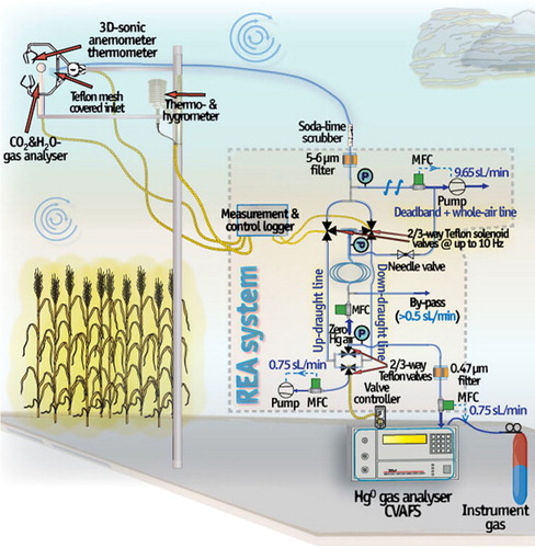
Continuously, air was drawn at 10.4 sL min⁻¹ through an intake positioned ~15 cm from the path of a 3D-sonic anemometer (C-SAT3, Campbell Scientific). After passing 2.47 m through the 3.99 mm (5/32″) ID PFA tubing, a subsample at 0.75 sL min⁻¹ of this flow is routed by two fast-response (opening and closing times<50 ms) three-way solenoid valve with Teflon as wetted surface material (NResearch Inc. Model 648T031, coil power ~8 W or BECO Manufacturing Co. Inc. Type 443W1DFR-LT, coil power ~5 to 6 W) to either up- or downdraught sampling lines. As inferred by Nie et al. (1995), it is preferential to maintain a high flow rate in case of a single intake line, where the up- and downdraught air resides as adjacent plugs, to reduce available time for longitudinal smearing being critical for small eddy parcels. The flow in our whole-air sampling line would plausibly be classified as turbulent since Reynold's number critical for the transition to a regime including spreading turbulent elements (Re~2040, Avila et al., 2011) was exceeded (Re~3500). Turbulent transport is favourable in suppressing conditional parcel mixing (Lenschow and Raupach, 1991; Massman, 1991). The conditional valves are controlled by a data logger (CR3000, Campbell Scientific) that acquired 10-Hz wind speed data from the anemometer and computes a 5-minute running average of the vertical wind speed updated every 30 s used as the conditional threshold (), then delay the 12 V execution signal to valve until the air parcel arrived. The corresponding effective lag time (~0.3 s) was computed separately in a differential experiment from the maximum cross-correlation between w and CO₂ using 10-Hz data of CO₂ concentration from an infrared open-path CO₂/H₂O gas analyser (IRGA, LI-7500A, LI-COR Biosciences) following the procedures of Ruppert (2005). This lag time was taken into account in the REA-OPEC control programme written for the data logger and also corresponds within experimental resolution (100 ms) to the inlet tube delay time calculated from flow and geometric considerations.

Up- and downdraught sampling was carried out using as discriminator instead of w=0 to prevent slight inaccuracies in the levelling of the sonic anemometer and lateral irregularities in the sampling fetch bias sampling (cf. Section 3.3). In addition, the system was optionally operated with a dynamic velocity deadband ( where b typically 0.1–0.3). In that case, if , neither valve was activated. Accounts providing information about the effect and benefits of using a deadband in REA can be found elsewhere (Ammann and Meixner, 2002; Grönholm et al., 2008). The relaxation coefficient for a deadband application is in relation to that of a zero-deadband () according to Businger and Oncley (1990) of the magnitude .

Both conditional sampling valves were connected with their normally opened ports to a supply of air scrubbed of Hg (c_ZA≤0.1 ng sm⁻³ Hg⁰, model 1100 Zero Air Generator, Tekran Instruments) hooked up in a by-pass configuration to vent a surplus of injected air. Hg-zero air is thus delivered at 0.75 sL min⁻¹ to the conditional line(s) that at the moment is not activated for sampling. This approach improves the sampling flow stability by dampening switch transients. However, if there exists significant pressure differentials across the upstream ports of a conditional valve (e.g. between the zero air injection and high gas flow section), flow irregularities will nevertheless be present. Pressure was monitored by three wireless pressure transmitters (DPG409 series, Omega Engineering Inc.) operated at 2.5 Hz with positions given in Fig. 1. Using an arrangement similar to Schade and Goldstein (2001), the zero air pressure was adjusted to match the subambient one in the upstream zone of the fast-response segregator valves (cf. Section 3.3).

The REA-OPEC programme includes options to disable conventional REA sampling and permit operation in either static (valves off: zero air sampling or valves on: whole ambient air sampling) or dynamic (whole air excluding sampling within a deadband±w₀) mode in order to assess potential systematic bias between the two conditional sampling lines. Reference sampling forms the basis for correcting channel bias (see Section 2.3, eqs. 4–5).

By using a combination of two three-way solenoid valves (cf. Fig. 1), executed by a controller with electronic drivers (Tekran 1110 Two Port Sampling System) synchronised with the sampling cycles of an automated Hg vapour analyser (Tekran 2537B), one conditional sample line was opened to the analyser while the other was pumped out of the system (Cobos et al., 2002; Bash and Miller, 2008). High-precision mass flow controllers (MFC, a MilliPore-Tylan FC 280 inside the 2537B instrument and externally three Brooks Instrument SLA5851) were used for maintaining consistent flow rates. MFC flow rate readings were logged by a Brooks Instrument 0254 device and acquired on a computer for later evaluation.

The 2537B instrument utilised two gold trap cartridges in parallel, with alternating operation modes (sampling and desorbing/analysing in mercury-free Ar stream) to continuously determine Hg⁰ concentration on a predefined time base of 5 minutes. The performance of the cartridges was routinely checked by injections from internal and external temperature-controlled mercury sources. The mercury vapour analytical instrument is sensitive to limited power and the analyser was therefore always supplied with grid or generator power passing a 10-kW voltage stabiliser to ensure proper operation in the field. To eliminate potential bias in the performance between gold traps, two consecutive 5-minutes measurements were performed on the same up- or downdraught reservoir before switching to the other. Consequently, a minimum period of 20 minutes was required to obtain a single flux from concentration measurements (eq. 1).

Concerning MM data (collected at 10 Hz), most land–atmosphere exchange studies have adopted time periods of between 10 and 60 minutes as the averaging interval to calculate flux means (Moncrieff et al., 2004). For the final evaluation of our REA system in the field, the integration interval of 20 minutes was found to be adequate for flux computation (Section 3.1). Individual concentration measurements of Hg⁰ in the up- () and downdraught () reservoir requires correction for the dilution by injection of zero air to represent the corresponding true concentrations () and () respectively in the conditional sampled eddies according to:

where α_↑ and α_↓ represent the fraction of time the up- and downdraught sampling valves activated. The detection limit of the Hg⁰ analyser was≤0.15 ng m⁻³ for a 5-minute sample calculated as 2σ. The overall uncertainty of air Hg⁰ measurements was estimated at ±5% (2σ) using the procedures described in Temme et al. (2007). For the application of REA, the precision of the instrument is the most important, rather than the accuracy. It is therefore preferable to use the same analysing unit for up- and downdrafts rather than independent mercury vapour analysers. However, the involvement of asynchronous (sequential) collected of up- and downdraught samples in the process introduces errors at times of short-time variation in ambient air Hg⁰ concentration and turbulence relative to the 20-minute averaging interval. The latter issue was addressed by meteorological quality tests (see Section 2.2.3). Bias between sampling lines wetted by conditional samples may exist and prompts for regular check upon (see Section 3.3). Tubings installed in these sampling lines were fresh and flushed with zero air before use. Fittings and valves were subject to hot acid treatment, rinses in Milli-Q water and dried in a stream of zero air before being assembled.

In addition to the 3D-sonic anemometer required for REA measurements, the IRGA and an HMP155 temperature and humidity probe (Vaisala, Finland) enabled OPEC measurements of CO₂ (), latent heat (), buoyancy (), momentum and computed sensible heat () flux. The IRGA was mounted 0.15 m below the anemometer (z _m =2.05 m) and displaced 0.15 m laterally to the predominating wind direction justified to minimise high-frequency flux loss due to vertical (Kristensen et al., 1997) and longitudinal (Massman, 2000) sensor separation. Moreover, the IRGA was slightly tilted to facilitate drainage of droplets on its optical windows after precipitation events. Using the approximation of Raupach (1994): , it was inferred that the position of OPEC sensors was well above the roughness sublayer height (z _*) and thus within the preferred surface layer. 10 Hz data were sampled and stored with the CR3000 data logger equipped with flash memory storage device (SC115, Campbell Scientific) for hourly backup. OPEC fluxes were computed as:2

where represents the average dry air density, w′ and variations around the temporal mean of vertical wind velocity and the mass mixing ratio of the scalar of interest (for momentum , for buoyancy and for latent heat flux ) and the overbar represents the 20-minute averaging time. Furthermore, u is the longitudinal wind velocity, T _s is the air temperature measured by the sonic anemometer, c _p is the specific heat of air at constant pressure, q is the specific humidity and λ is the heat of evaporation for water. From the measurements of momentum flux, friction velocity () was derived.

The MM REA-OPEC measuring complex was accompanied by a weather station (HOBO U30-NRC, OnsetComp., USA) equipped with sensors for bulk air (temperature and humidity), surface soil (temperature, volumetric moisture content) parameters and canopy leaf wetness as well as sensors for solar radiation (300–1100 nm) and photo-synthetically active radiation (400–700 nm), respectively.

2.3. Post-processing, correction methods, averaging times and quality assessment of flux data

Post-processing of 10 Hz OPEC data stored on the SC115 device using the open-source EddyPro™4.0 flux analysis software package (LI-COR Biosciences Inc.) was performed for the following data corrections: time lag compensation by covariance maximisation (Fan et al., 1990), double axis rotation method for compensating for tilt (Kaimal and Finnigan, 1994), buoyancy flux corrections (van Dijk et al., 2004), air density fluctuation correction for latent heat and CO₂ flux (Webb et al., 1980) and frequency response corrections with high- and low-pass filters (Moncrieff et al., 1997, 2004). Moreover, data were quality controlled by testing for steady state (stationarity, ST) and integral turbulence (ITT) (Foken and Wichura, 1996; Hammerle et al., 2007). For ITT, deviations from the Monin–Obukhov-similarity-theory were tested by comparing theoretical (modelled) values of the stability function for vertical velocity () following Kaimal and Finnigan (1994) with measured ratios of σ _w to u*:

L is the Obukhov length, κ is von-Kármán's constant (~0.41), g is the acceleration due to gravity. The presence of steady-state conditions was tested by comparing the 20-minute average of covariance with the four consecutive 5-minute covariances in the same time period . Based on ST and ITT, an overall quality flag (according to the three grade 0–1–2 system scale described in Mauder and Foken, 2004) was assigned to the 20-minute averaged u _*, ,, and . The frequency response of the REA-OPEC system at the YCES field site was investigated by spectral analysis of selected 10-Hz turbulence time series. Normalised and exponentially bin-averaged (50 bins in normalised frequency domain , where f is the frequency and is the mean horizontal wind speed) cospectra () and cumulative integral of cospectra beginning with the highest frequencies (, Foken and Wichura, 1996) were computed for T _s and . Ogive (Og) functions computation was extended to low frequencies f ₀~10⁻⁴ Hz by using up to 2-hour block averaging time. Hence, the contribution from the low-frequency part of fluxes could be assessed to determine an averaging time required to obtain reliable fluxes.

The Hg⁰-REA-CVAFS system included MFCs calibrated with dry air to represent conditions at STP (0°C and 1013.25 hPa) and therefore raw Hg⁰ flux (, ng m⁻² h⁻¹) data from eq. 1 require correction for the effect of ambient air moisture and temperature. An appropriate correction formula for flux obtained by MM methods including conventional-type MFCs was implemented following Lee (2000):3

where is the corrected Hg⁰ flux, R _d is the ideal gas law constant for dry air, P ₀ and T ₀ is the pressure and temperature at STP respectively, is the average ambient air Hg⁰ mass concentration over the flux averaging interval and is the water vapour flux.

Regularly, the REA system was operated in reference sampling mode (opening and closing both the up- and the down-inlet at the same time with a dynamic velocity deadband as a threshold) to correct for minor bias between the conditional channels according to:4

and5

where and are the uncorrected concentration level and the concentration level obtained in reference mode for either the up- (↑) or downdraught (↓), respectively.

Footprint analysis was used for predicting the size of the source area and hence clarified if the measured flux was representative for the target grain fields. We employed the scaling approach by Kljun et al. (2004) for conditions within its specified limitations (−200≤ζ≤1, u*≥0.2 m s⁻¹), otherwise the analytical model developed by Kormann and Meixner (2001), both as part of the EddyPro™ software.

The empirical β-factor used in eq. 1 was derived in situ from suitable scalars s those can be measured by OPEC as well as by REA simulations (, and ) during an experiment according to:6

where is the difference between the specific scalar quantity in up- and downdraught, respectively during the 20-minute averaging period. Alternatively, as further discussed in Section 3.2, a mean β _s -factor () can be determined as the slope in a plot of versus .

3. Characterisation of the Hg⁰-REA-CVAFS system

3.1. Sensor response and optimisation of averaging time

In Fig. 2, normalised cospectra of buoyancy and CO₂ flux are presented being ensemble means for the periods of unstable conditions at the YCES field site together with that derived from a model proposed by Kaimal et al. (1972) at appropriate stability and height. In Fig. 2, the ‘Kaimal cospectra’ aligns in the high-frequency inertial subrange (f _z ~1−10) asymptotically to a linear slope of −4/3 predicted by Kolmogorov's laws. The buoyancy flux obtained from a single sensor followed as expected the ideal slope for this frequency decade while the CO₂ (and H₂O) flux was significantly dampened. Correction for high-frequency gas flux loss was in a first step computed by EddyPro™ software and in a later step spectral correction on sensible heat flux was implemented. Considering f _z <1, there were no detectable differences between the CO₂ and temperature curves in Fig. 2 indicating insignificant cospectral distortion. This is also evident from ogive (Og) tests performed on averaging periods extending to 2 hours (cf. Fig. 3).

Fig. 2 Cospectra of vertical wind speed (w) with CO₂ (yellow filled circles) and sonic temperature, T (red filled circles) based on the daytime data from YCES with unstable conditions. As a reference, the corresponding Kaimal model cospectrum is displayed (dashed curvature) as well as the −4/3 slope (filled purple line) expected from Kolmogorov's theory.

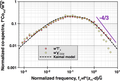
Fig. 3 An ogive calculated for 12:00–14:00, May 10, 2012 at YCES.

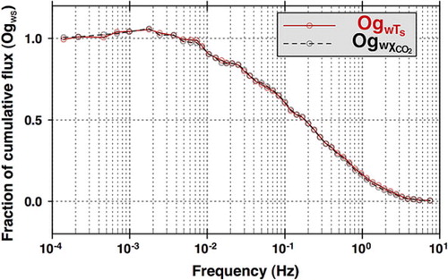
In a clear majority (~90%) of the investigated cases (daytime data), ogive curves reached an asymptote or attained a global maximum within the 10–20 minute cycle interval (~0.001 Hz) implying that 20 minutes is adequate for flux computation. By using a comparatively short averaging time, the inclusion of non-turbulent trends may be avoided (Ammann, 1998). This conclusion compares favourably with that of turbulence observations at low surface layer heights in many flat cropland studies (Baker et al., 1992; Kaimal and Finnigan, 1994) and is consistent with the previous findings of Sun et al. (2005) over crop fields at YCES. An inspection of recorded turbulence cospectra indicates that our REA-OPEC system is capable of measuring turbulence scalar fluxes via its OPEC mode.

3.2. β_s – factor evaluation and conditional sampling statistics

The algorithms used in REA for calculating trace gas fluxes are based on the assumption of similarity of the turbulent exchange of scalar quantities (Kaimal et al., 1972) as well as of flux and variance (Wyngaard et al., 1971). Particularly for the derivation of β-factor, the scalar similarity is required. In the surface layer, factors derived from experimental studies are generally lower than the ideal value of , typically being reported on an average of 0.51–0.62 due to the non-Gaussian nature of turbulence (Businger and Oncley, 1990; Oncley et al., 1993; Gao, 1995; Katul et al., 1996; Ammann and Meixner, 2002). Furthermore, β _s displays a significant short-time variation (Oncley et al., 1993; Grönholm et al., 2008), which potentially restricts the use of a fixed value (e.g. derived from linear regression fitting of plots versus at being deployed for extensive time series REA flux calculations (Oncley et al., 1993; Pattey et al., 1993).

In Fig. 4, -factors derived from eq. 6 utilising the observations from LGR as well as YCES field experiments (each of ~1000 averaging periods in size) are displayed as a function of the corresponding OPEC fluxes. Whereas the YCES data have been segregated into the three quality classes as described in Section 2.3, the measuring system at the time of the LGR experiment lacked the capability to store 10-Hz raw data on a daily basis and therefore are in this case displayed as the bulk. As can be seen in Fig. 4, there is a considerable scatter in particularly when the reference flux approaching zero (n.b. in the divisor of eq. 6 becomes minor). This happens when the scalar flux changes sign or diminishes to near zero in the morning and evening hours and during the night, respectively. Given this methodological problem, the LGR data were screened from the lowest 5% range of absolute flux observations (Ammann and Meixner, 2002).

Fig. 4 β-factor () as a function of scalar fluxes over a grassland (left column) and winter wheat stand (right column) fetch. Upper panel: latent heat flux, middle panel: buoyancy flux, lower panel: CO₂ flux. In all of the panels, some data are positioned outside the plot range. The data from YCES was segregated into three quality classes based on turbulence tests (see Section 2.3).

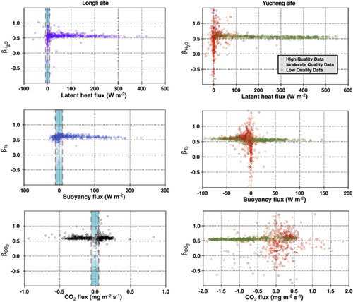
Omitting the data for < 10 W m⁻², <12 W m⁻² and <0.08 mg m⁻² s⁻¹ (shaded intervals in Fig. 4), the simulated statistics described as median±1.48 interquartile range (IQR) was =0.564±0.060, =0.574±0.062 and =0.571±0.069, respectively. For the YCES -factors, there was a tendency for statistical dichotomy between data with high quality and data with lower quality. In particular for heat, low-quality data were largely associated with low fluxes. -factors derived from the high-quality turbulence YCES data (comprising ~56% of the total) were all of very similar medians around 0.56 (= 0.562±0.051, = 0.569±0.055 and = 0.558±0.092).

Consequently, during methodologically favourable conditions with respect to turbulence, there was negligible difference between -medians of the scalar investigated. The corresponding median of 0.56±0.01 concurs very well with the literature data reported from similar settings (Baker et al., 1992; Pattey et al., 1995; Beverland et al., 1996; Hamotani et al., 1996; Katul et al., 1996; Ammann and Meixner, 2002), thus confirming that our system simulates REA parameters from OPEC data as expected.

A related issue is the statistics of conditional sampling. In Fig. 5, the time series at YCES of percentage proportion of downdraught sampling () is displayed segregated by the individual data quality classes. Since the REA system was operated with no deadband application, ideally 1:1 distribution between up- and downdraught sampling was expected. This was true for the distribution ( 0.507) associated with high-quality data. However, for lower turbulence quality classes, -ratios deviated in most cases significantly from unity. At night, significant to extreme predominance of sampling into either of the channels was prevailing for longer periods. Such periods were associated with very calm (u _*< 0.05 m s⁻¹) and near-neutral to slightly stable conditions (0.3>ζ>−0.2) with dampened turbulence. This prompts for on-line processing the w-signal in a more elaborate way during nighttime by promoting swifter conditional valve switching. Thus, it appears justified and necessary to classify REA data using high-quality turbulence index as the criterion. This has previously not been implemented in Hg⁰ air-surface exchange studies using the REA technique (Cobos et al., 2002; Olofsson et al., 2005; Bash and Miller, 2008). In turn, as advocated by Bowling et al. (1998), we chose to utilise a running in eq. 1 rather than a fixed β _s from regression for periods of high-quality turbulence and only the latter () for remaining periods of data.

Fig. 5 Daily courses of the distribution () of downdraught sampling with respect to quality indexed groups (high-quality green circles, moderate quality yellow diamond and low-quality red squares).

3.3. Assessment of bias in conditional sampling

3.3.1. Observance of the constant flow rate criteria of REA

Experimental control of the conditional sampling flow is not viable with regular mass flow controllers due to their typical response times in the order of 1 s (manufacturer specification: 1 s to reach within 2% of the set point), which is as aforementioned within the typical time interval of conditional valve switching. However, supplementary pressure measurements are fast enough for the examination and adjustment of flow fluctuations. The REA criterion of constant flow rate through conditional channels in open state can in practise be maintained only if pressure equality is approached over the ports of the conditional sampling valves.

In Bash (2006), mass flow controller/meter logs of cumulative volume were used to determine if flow fluctuations were present. While a Hg-zero air injection was applied, Bash and Miller (2008) reported without noting any further pressure control measures that very minor flow rate fluctuations (<±0.1% of the set point) occurred in their system. Given the position of the conditional valves in our system, injection of zero air at atmospheric pressure led to significant variability in conditional sampling flow rate, albeit MFC logs of cumulative volume indicated desirable values (e.g. 3.75±0.01 sL for each 5-minute sample). An example of a typical time series of such non-constant conditional sampling flow is illustrated in the left panel of Fig. 6. As seen, sudden pressure changes cause flow surges and biased sampling of the analyte of interest. However, if sample and zero air pressure were adjusted to roughly equal values, the flow rate characteristic downstream the conditional valves was significantly improved (Fig. 6, right panel). With the guidance of the set of pressure sensors, an operator can minimise pressure differentials by adjusting the flow rate of zero air with a needle valve after the injection stream passed a few metres of PFA tubing (1.59 mm ID).

Fig. 6 Characteristics of the REA-CVAFS system without (left column) and with the use of pressure adjusted Hg-zero air injection (right column). For each case, typical time series for daytime unstable conditions are given for w (upper panels, 10 Hz), line pressures (middle panels, 2.5 Hz) and mercury analyser sampling inlet flow rate (lower panels, 1 Hz).

3.3.2. Zero and channel inter-comparison in reference sampling mode

Tubings, fittings, filters and valves included in the REA system's joint and conditional sampling lines were regularly investigated for contamination/carry-over bias. Checks in the valves off mode did not reveal measureable artefacts: the Hg⁰ signal measured from zero air passing the conditional lines was inseparable from that of the zero air generator outlet. Checking the measured Hg⁰ concentrations in the up- and downdraught channels when the REA system was deactivated by running in valves on stasis likewise also yielded relatively constant , which statistically equalled zero. However, channel inter-comparison by acquiring identical samples from the process of opening and closing the conditional valves simultaneously (Section 2.2) indicated minor systematical channel bias to proceed (Supplementary file). The conditional concentration data were corrected using eq. 4 and 5 following the reference sampling mode carried out for 2 hours every 48–72 hours REA sampling interval. To simulate concurrent Hg⁰ measurement of the channels during the reference sampling, continuous sets were constructed from sequential data series by cross-interpolation.

3.4. Sonic anemometer inflow conditions and flux footprint estimation

Distribution of wind direction (Supplementary file) clearly shows that typical conditions at YCES were characterised by south–south-westerly winds. The preferred inflow sector (±90°) relative to the sonic anemometer head, which pointed at ~200° thus aligned favourably to most of the wind conditions (mean direction 199°). About 33% of the daytime data (6:20–19:20) fell outside this sector while the corresponding figure for nighttime was 14%. Moreover, used as a conditional sampling threshold appear insignificantly biased from zero under any of the wind direction encountered. Normalised daytime values () were computed and averaged for 30° per bin wind direction, whereby the sector means were found to fall within a range of small offsets (−0.12–0.15) from zero.

Fig. 7 Polar histogram of 20-minute averaged 5° per bin Hg⁰ conc. (ng sm⁻³) classified into four magnitude levels (a. left). Diurnal variation of Hg⁰ concentrations is represented as a notched box &whiskers percentile plot (b. right). The end of the whiskers represents the 10^th and 90th percentile respectively while the half width of the notches is calculated by , where n is the number of samples. Mean is indicated by filled diamonds.

The position and dimension of source area contributing to the flux measurement were approximated for each averaging interval. This flux footprint is strongly dependent on atmospheric stability. For daytime data, the distance from sensor predicted to give the maximum relative individual contribution to the flux () was at 18±7 m. In turn, (predicted mean distance ≤70% of the flux derived) was at 49±34 m and the corresponding was at 130±125 m. For a comparison of the source area dimensions, a view of the fetch length with major objects contrasting to wheat grain field is overlaid in Fig. S1. In ~72% of the cases, daytime REA-OPEC-flux 90% isopleth footprints lay within undisturbed fields of target. During nighttime, the footprint dimension was generally more extensive and even (188 m) exceeded in the dominating wind sector, the water course and fell in the wheat field to the south of it. The total Hg content in surface soils was uniform across the measurement fetch (mean: 45±3 ng/g, n=29).

4. Field application

4.1. General meteorological conditions at YCES

The REA-OPEC system described above was deployed for trial Hg⁰ flux measurements from 2 to 18 May 2012. The general meteorological conditions at YCES were characterised as fair and moist (median RH ~91.6%) without significant precipitation (0.2 mm) and air pressure fluctuations (▵p ~13 hPa). The ground wind flow was mainly from S to SW with occasional counter-current flow (NE–E) associated with raising air pressure. The air temperature ranged from 10 to 30°C, whereas the volumetric soil water content at ~10 cm depth exhibited small diurnal features overlaid on a declining trend from 0.23 to 0.11 m³ m⁻³, significantly inferior to the field capacity of 0.44 m³ m⁻³ (Li et al., 2010). The degree of canopy leaf wetness showed a strong diurnal variation, which during calm nights may reach a protracted maximum of unity from about dawn to dusk time.

4.2. Surface layer air Hg⁰ concentration level

In Fig. 7, the angular and diurnal distribution of 20 minute averaged ambient observed air Hg⁰ concentration is displayed. Hg⁰ at YCES exhibited a wide range (2.04–12.67 ng sm⁻³) with a median of 4.85 ng sm⁻³, which is clearly elevated above that of the hemispherical background. Nevertheless, the data are comparable with observations made in inland China (Fu et al., 2012a). As seen in Fig. 7a, there is no clear dependence of Hg⁰ concentration on wind direction, implying the contribution of regional rather than local Hg pollution sources to the observations. This region of China is heavily industrialised and includes significant point sources, such as coal combustion, chemical-construction material manufacture and metal smelting facilities, and so on. Hg⁰ observations followed a marked diel convolution with a near mid-day high and shallow nighttime minima bottoming out at 2.5–4 ng sm⁻³. The sharply increasing Hg⁰ concentrations during the daylight morning hours might have largely stemmed from mixing-in of more Hg⁰-rich air from aloft plausibly including the break-up of inversions.

4.3. Air-surface Hg⁰ exchange characteristics

The Hg⁰ flux time series is shown in Fig. 8 together with the corresponding cumulative flux. In the plot, the turbulence quality classes are indicated by the flux markers’ colours. The flux data include both periods of emission and deposition and exhibit a positive distributional skewness and negative kurtosis indicating that the contribution from distribution tails to be rather important with emphasis on the right (evasion). A Shapiro–Wilk test rejected the hypothesis of normality of the flux distribution (p<0.001), suggesting that statistical estimators, such as median and 1.48 IQR, are capable of describing its location and scale.

Fig. 8 Time series of 1-hour averaged Hg⁰ flux (ng m⁻² h⁻¹, filled circles with colours based on turbulence quality classes, See Fig. 5) and corresponding cumulative flux (µg m⁻², blue solid line) over the experimental period at YCES.

The net Hg⁰ flux over the period was positive (61.2±340.2 ng m⁻² h⁻¹) with strong temporal variability. The observed range (−716.5–1005.2 ng m⁻² h⁻¹) is consistent with those of most other MM studies of Hg⁰ flux over croplands reported in the literature (Carpi and Lindberg, 1997; Gustin et al., 1999; Cobos et al., 2002; Kim et al., 2002, 2003; Cobos, 2003; Olofsson et al., 2005; Schroeder et al., 2005; Cobbett and van Heyst, 2007; Baya and van Heyst, 2010). For instance, Kim et al. (2003) observed Hg⁰ fluxes varying from −139 to 1071 ng m⁻² h⁻¹ overall during two spring campaigns over rice paddy fields in coastal Korea (~600 km E of YCES). Our median net Hg⁰ flux falls in between those of Kim et al.'s 2001 and 2002 campaigns (111 and −6 ng m⁻² h⁻¹), somewhat higher compared to those reported in related studies in North America. This could be due to a small section of the growing season covered by our data. Nevertheless, ongoing cropland experiments should generate multi-seasonal data warranting for a more profound analysis. The overall correlation (ρ, Spearman's rank-order correlation coefficient) between Hg⁰ flux and other measured parameters during the bi-weekly experiment at YCES were generally weak to moderate (ρ ²<0.2) with the exception in some measure to u_*, wind speed and ambient air Hg⁰ (cf. Fig. 9). This corresponds with several related MM studies (Lee et al., 2000; Bash and Miller, 2009; Converse et al., 2010), which report correlations minor in magnitude with environmental parameters, which in turn exhibit specific seasonal signatures. The relationship of environmental variables with the Hg⁰ flux may shed some light on processes driving the flux and is discussed in a brief qualitative way in the following.

Fig. 9 Heatmap matrix plot of Spearman's rank-order correlation coefficients (ρ) between Hg⁰ concentration, Hg⁰ flux and environmental variables. The absolute value of ρ is indicated by a colour code explained in the legend. Circles indicate a positive correlation while square markers represent a negative one. The scale of a marker is proportional to ρ ². Cells above the matrix diagonal refers to the statistical significance (p) of ρ. Significance levels p<0.05, p<0.01 and p<0.001 are indicated by *, * and *** respectively while a value p ≥ 0.05 is stated explicitly.

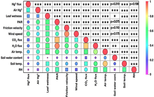
Recapitulating Section 4.2, it is apparent that the YCES sampling site is intermittently affected by the advection of Hg polluted air. A major Hg⁰-rich plume incursion occurred during several hours on May 9 with maximum concentration observed around mid-day. During this event associated with moderate winds turning easterly at dawn, major dry deposition of Hg⁰ (of a magnitude of up to ~720 ng m⁻² h⁻¹) was observed. The data set also covers other episodes, during which flux direction changing with ambient concentration levels are evident (Fig. 10). Overall, Hg⁰ flux showed moderate negative correlation with ambient air Hg⁰ concentration (ρ=−0.38, n=377).

Fig. 10 Time series of selected environmental and meteorological parameters measured at YCES. Panel a: Hg⁰ flux (red, left) and air Hg⁰ concentration (blue, right); panel b: friction velocity u* (red, left) and canopy leaf wetness degree (blue, right); panel c: PAR (red, left) and air temperature (blue, right); panel d: H₂O flux (red, left) and CO₂ flux (blue, right).

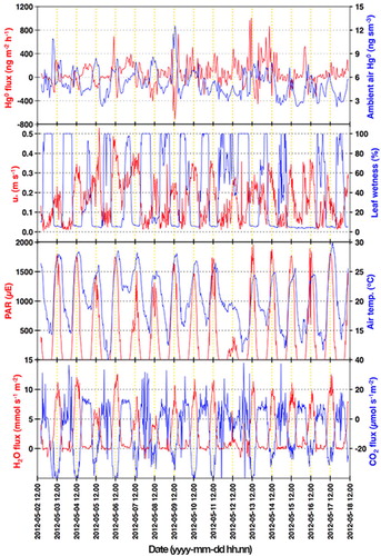
The median of night- and daytime Hg⁰ flux observations differed significantly (p<0.01, Mann–Whitney U-test) with the former smaller (9.8 vs. 77.1 ng m⁻² h⁻¹, respectively). As a composite, however Hg⁰ flux variation at YCES exhibited a much less regularly featured diurnal profile than, for example, that for CO₂ and H₂O flux (Fig. 10). In the literature, strong diurnal cycles have been reported for Hg⁰ flux determined over natural surfaces (daytime emissions – flux fluctuating near zero at night; Lindberg et al., 1998; Gustin et al., 1999; Cobos et al., 2002; Kim et al., 2002; Bash and Miller, 2008; Fritsche et al., 2008; Smith and Reinfelder, 2009; Baya and van Heyst, 2010; Converse et al., 2010).

In addition to the episodes of dry deposition in conjunction with advection of Hg polluted air, some disparate Hg⁰ emission patterns were observed during the daytime: when the leaf wetness sensor indicated a rapid dry-up of canopy in the morning hours (May 3–4, 6, 11, 13), (a) sharp emission peak(s) occurred. This can be interpreted as an effect of rapid photo-reduction of previously deposited Hg^II to Hg⁰ on foliage surfaces or into soil in conjunction with the presence of a water film and emerging incoming solar radiation (Graydon et al., 2006). The release of Hg⁰ may also be driven by the opening of stomatal apertures and onset of evapotranspiration (Kothny, 1973). Some other days (May 5, 7 and 14) with strong turbulence extending into dark hours, which in turn exhibited low (non-saturated) degrees of leaf wetness and considerably warm temperatures (‘tropical night’), the emission profile was broad and predominating through the night into the next day. As can be noticed in Fig. 8, these events led to a significant boost to cumulative Hg⁰ flux.

Concurrent measurements at the base of the wheat canopy using a DFC of novel design (Lin et al., 2012) revealed the presence of considerable soil surface emission following a regular diel pattern (mid-day maximum and nocturnal minimum close to zero flux). Hence, the air-canopy Hg⁰ fluxes measured by REA technique at YCES are likely to include a significant contribution deriving from ground-level Hg⁰ gas exchange. At present, the data set obtained thus far is too small to specifically address the processes controlling the cropland air-surface exchange of Hg⁰. However, ongoing seasonal field experimental work, which in addition include measurements of Hg content in soil and foliage as well as deposition, should warrant a discussion in a forthcoming communication.

5. Conclusions

An REA-CVAFS system has been designed and developed for the measurement of Hg⁰ vapour air-surface exchange. The performance of the fully developed system was evaluated by inter-comparison with an OPEC CO₂–H₂O flux system over essentially horizontally homogeneous settings (nearly-mature winter wheat canopy and grazed grassland, respectively). Fluxes of latent heat, buoyancy and CO₂ measured by EC and synthesised by the REA algorithm yielded during developed turbulence median -factors of 0.56±0.01, in good agreement with literature data. The REA system was synchronised (i.e. match of the delay between the wind speed measurement and corresponding conditional sampling), and the time shifts in w-CO₂ cross-correlation were determined as a function of tube length sampled at constant flow rate. The configuration of fast-response sampling valves permitted zero- and whole-air to be flushed through conditional channels dynamically. Such reference sampling was used for correcting for bias that may exist between the channels.

In contrast to the Hg⁰-REA system designs previously reported in the literature (Cobos et al., 2002; Olofsson et al., 2005; Bash and Miller, 2008), the REA system described in this study allows the combined usage of a single Hg⁰ gas analyser, injection of zero air to dampen sampling flow disturbances introduced by conditional valve switching, and the disposal of sampled air when it is small (‘deadband’). Furthermore, departures from the constant sampling flow criterion of REA, which can be most severe in systems without any specific deadband channel, were addressed by implementing control of sampling line pressure.

6. Acknowledgments

This study was supported by the State Key Laboratory of Environmental Geochemistry and the National Basic Research Program of China (2013CB430002) as well as by the Chinese Academy of Sciences through an instrument development programme (YZ200910) and the Natural Science Foundation of China through grants 41030752 and 40825011. The technical staff of Yucheng station is greatly appreciated for the facilities and infrastructure kindly made available to us.

Notes

To access the supplementary material to this article, please see Supplementary files under Article Tools online.

7. Appendix

Nomenclature

Table

Symbol	Meaning	Unit
	Turbulent water vapour flux (measured by EC)	g m^−2 s^−1
	Turbulent latent heat flux (measured by EC),	W m^−2
	Turbulent buoyancy flux (measured by EC)	W m^−2
	Turbulent sensible heat flux (measured by EC)	W m^−2
	Turbulent carbon dioxide flux (measured by EC)	mg m^−2 s^−1
	Turbulent elemental mercury vapour flux (measured by REA)	ng m^−2 h^−1
Co ws	Cospectral density of w and s	^1
Og ws	Ogive function	^1
	Mass concentration (density) of elemental mercury vapour	ng m^−3
c p	Specific heat of air at constant pressure	J kg^−1 K^−1
d	Displacement height	m
f	Frequency	s^−1
f z	Normalised frequency	^−
g	Acceleration due to gravity	m s^−2
h	Canopy height	m
L	Obukhov length	m
P	Pressure	Pa
P 0	Standard pressure (1013.25 hPa)
q	Specific humidity	kg kg^−1
R d	The ideal gas law constant for dry air	J kg^−1 K^−1
Re	Reynolds number	–
T	Air temperature	K
T 0	Standard temperature (273.15 K)
T s	Sonic air temperature	K
u	Longitudinal component of the wind velocity	m s^−1
u *	Friction velocity	m s^−1
w	Vertical component of the wind velocity	m s^−1
w 0	Magnitude of deadband for REA method	m s^−1
x	Horizontal direction parallel to the average wind velocity/fetch	m
	Mean of the scalar x	^1
	Predicted value of scalar x	^1
z	Height	m
z *	Height of the roughness sublayer	m
z 0	Roughness height/length	m
z m	Measurement height	m
a	Fraction of time of up- and downdrafts to the total sampling time: and respectively.	–
	Relaxation coefficient used in REA measurements without deadband application obtained from OPEC and REA simulations of a specific scalar s	–
	Relaxation coefficient used in REA measurements with a deadband application w0 obtained from OPEC and REA simulations of a specific scalar s	–
z	Dimensionless height (z m –d)/L	–
k	Von Kármán's constant (~0.41)	–
λ	Latent heat of vapourisation for water	J kg^−1
ρ	Spearman's rank-order correlation coefficient	–
ρ d	Air density (dry)	kg m^−3
σ	Standard deviation	^1
σ w	Standard deviation of vertical wind speed	m s^−1
χ s	Mass mixing ratio of scalar component s	kg kg^−1

1 Dimension according to the use of the parameter.

References

- Ammann C . On the Applicability of Relaxed Eddy Accumulation and Common Methods for Measuring Trace Gas Surface Fluxes. 1998; Zürich, Switzerland: Swiss Federal Institute of Technology (ETH). 229. PhD Thesis.
- Ammann C , Meixner F. X . Stability dependence of the relaxed eddy accumulation coefficient for various scalar quantities. J. Geophys. Res. 2002; 107: 4071–4080.
- Avila K , Moxey D , de Lozar A , Avila M , Barkley D , co-authors . The onset of turbulence in pipe flow. Science. 2011; 333: 192–196.
- Baker J. M , Norman J. M , Bland W. L . Field-scale application of flux measurement by conditional sampling. Agr. Forest Meteorol. 1992; 62: 31–52.
- Bash J. O . Measurements of Total Mercury Flux Over a Forest Canopy for Model Development. 2006; Storrs, CT: University of Connecticut. 166. PhD Thesis.
- Bash J. O , Miller D. R . A relaxed eddy accumulation system for measuring surface fluxes of total gaseous mercury. J. Atmos. Ocean Tech. 2008; 25: 244–257.
- Bash J. O , Miller D. R . Growing season total gaseous mercury (TGM) flux measurements over an Acer rubrum L. stand. Atmos. Environ. 2009; 43: 5953–5961.
- Baya A. P , van Heyst B . Assessing the trends and effects of environmental parameters on the behaviour of mercury in the lower atmosphere over cropped land over four seasons. Atmos. Chem. Phys. 2010; 10: 8617–8628.
- Beverland I. J , Oneill D. H , Scott S. L , Moncrieff J. B . Design, construction and operation of flux measurement systems using the conditional sampling technique. Atmos. Environ. 1996; 30: 3209–3220.
- Bowling D. R , Pataki D. E , Ehleringer J. R . Critical evaluation of micrometeorological methods for measuring ecosystem–atmosphere isotopic exchange of CO2 . Agr. Forest Meteorol. 2003; 116: 159–179.
- Bowling D. R , Turnipseed A. A , Delany A. C , Baldocchi D. D , Greenberg J. P , co-authors . The use of relaxed eddy accumulation to measure biosphere–atmosphere exchange of isoprene and of her biological trace gases. Oecologia. 1998; 116: 306–315.
- Businger J. A , Oncley S. P . Flux measurement with conditional sampling. J. Atmos. Ocean Tech. 1990; 7: 349–352.
- Carpi A , Lindberg S. E . Sunlight-mediated emission of elemental mercury from soil amended with municipal sewage sludge. Environ. Sci. Technol. 1997; 31: 2085–2091.
- Christensen C. S , Hummelshøj P , Jensen N. O , Larsen B , Lohse C , co-authors . Determination of the terpene flux from orange species and Norway spruce by relaxed eddy accumulation. Atmos. Environ. 2000; 34: 3057–3067.
- Ci Z , Zhang X , Wang Z . Enhancing atmospheric mercury research in China to improve the current understanding of the global mercury cycle: the need for urgent and closely coordinated efforts. Environ. Sci. Technol. 2012; 46: 5636–5642.
- Cobbett F. D , van Heyst B. J . Measurements of GEM fluxes and atmospheric mercury concentrations (GEM, RGM and Hg-p) from an agricultural field amended with biosolids in Southern Ont., Canada (October 2004–November 2004). Atmos. Environ. 2007; 41: 2270–2282.
- Cobos D. R . Determination of Mercury Vapor Fluxes by Conditional Sampling. 2003; St. Paul, MN: University of Minnesota. 141. PhD Thesis.
- Cobos D. R , Baker J. M , Nater E. A . Conditional sampling for measuring mercury vapor fluxes. Atmos. Environ. 2002; 36: 4309–4321.
- Converse A. D , Riscassi A. L , Scanlon T. M . Seasonal variability in gaseous mercury fluxes measured in a high-elevation meadow. Atmos. Environ. 2010; 44: 2176–2185.
- Desjardins R. L , Buckley D , St Amour G . Eddy flux measurements of CO2 above corn using a microcomputer system. Agr. Forest Meteor. 1984; 32: 257–265.
- Edwards G. C , Rasmussen P. E , Schroeder W. H , Wallace D. M , Halfpenny-Mitchell L , co-authors . Development and evaluation of a sampling system to determine gaseous mercury fluxes using an aerodynamic micrometeorological gradient method. J. Geophys. Res. 2005; 110 D10306.
- Fan S. M , Wofsy S. C , Bakwin P. S , Jacob D. J , Fitzjarrald D. R . Atmosphere–biosphere exchange of CO2 and O3 in the central Amazon Forest. J. Geophys. Res. 1990; 95: 16851–16864.
- Feng X. B , Tang S. L , Li Z. G , Wang S. F , Liang L . Landfill is an important atmospheric mercury emission source. Chin. Sci. Bull. 2004; 49: 2068–2072.
- Feng X. B , Wang S. F , Qiu G. A , Hou Y. M , Tang S. L . Total gaseous mercury emissions from soil in Guiyang, Guizhou, China. J. Geophys. Res. 2005; 110
- Foken T , Wichura B . Tools for quality assessment of surface-based flux measurements. Agr. Forest Meteorol. 1996; 78: 83–105.
- Fritsche J , Wohlfahrt G , Ammann C , Zeeman M , Hammerle A , co-authors . Summertime elemental mercury exchange of temperate grasslands on an ecosystem-scale. Atmos. Chem. Phys. 2008; 8: 7709–7722.
- Fu X , Feng X , Sommar J , Wang S . A review of studies on atmospheric mercury in China. Sci. Total Environ. 2012a; 421–422: 73–81.
- Fu X. W , Feng X. B , Wang S. F . Exchange fluxes of Hg between surfaces and atmosphere in the eastern flank of Mount Gongga, Sichuan province, southwestern China. J. Geophys. Res. 2008; 113
- Fu X. W , Feng X. B , Zhang H , Yu B , Chen L. G . Mercury emissions from natural surfaces highly impacted by human activities in Guangzhou province, South China. Atmos. Environ. 2012b; 54: 185–193.
- Gaman A , Rannik Ü , Aalto P , Pohja T , Siivola E , co-authors . Relaxed eddy accumulation system for size-resolved aerosol particle flux measurements. J. Atmos. Ocean Tech. 2004; 21: 933–943.
- Gao W . The vertical change of coefficient b, used in the relaxed eddy accumulation method for flux measurement above and within a forest canopy. Atmos. Environ. 1995; 29: 2339–2347.
- Goldstein A. H , Schade G. W . Quantifying biogenic and anthropogenic contributions to acetone mixing ratios in a rural environment. Atmos. Environ. 2000; 34: 4997–5006.
- Graydon J. A , St Louis V. L , Lindberg S. E , Hintelmann H , Krabbenhoft D. P . Investigation of mercury exchange between forest canopy vegetation and the atmosphere using a new dynamic chamber. Environ. Sci. Technol. 2006; 40: 4680–4688.
- Grigal D. F . Mercury sequestration in forests and peatlands: a review. J. Environ. Qual. 2003; 32: 393–405.
- Grönholm T , Haapanala S , Launiainen S , Rinne J , Vesala T , co-authors . The dependence of the beta coefficient of REA system with dynamic deadband on atmospheric conditions. Environ. Pollut. 2008; 152: 597–603.
- Guenther A , Baugh W , Davis K , Hampton G , Harley P , co-authors . Isoprene fluxes measured by enclosure, relaxed eddy accumulation, surface layer gradient, mixed layer gradient, and mixed layer mass balance techniques. J. Geophys. Res. 1996; 101: 18555–18567.
- Gustin M. S , Lindberg S , Marsik F , Casimir A , Ebinghaus R , co-authors . Nevada STORMS project: measurement of mercury emissions from naturally enriched surfaces. J. Geophys. Res. 1999; 104: 21831–21844.
- Hammerle A , Haslwanter A , Schmitt M , Bahn M , Tappeiner U , co-authors . Eddy covariance measurements of carbon dioxide, latent and sensible energy fluxes above a meadow on a mountain slope. Bound. Layer Meteorol. 2007; 122: 397–416.
- Hamotani K , Uchida Y , Monji N , Miyata A . A system of the relaxed eddy accumulation method to evaluate CO2 flux over plant canopies. J. Agr. Chem. 1996; 52: 135–139.
- Hicks B. B , McMillen R. T . A simulation of the eddy accumulation method for measuring pollutant fluxes. J. Clim. Appl. Meteorol. 1984; 23: 637–643.
- Hornsby K. E , Flynn M. J , Dorsey J. R , Gallagher M. W , Chance R , co-authors . A relaxed eddy accumulation (REA)-GC/MS system for the determination of halocarbon fluxes. Atmos. Meas. Tech. 2009; 2: 437–448.
- Jia L , Wang W. Y , Li Y. H , Yang L. S . Heavy metals in soil and crops of an intensively farmed area: a case study in Yucheng City, Shandong Province, China. Int. J. Environ. Res. Public Health. 2010; 7: 395–412.
- Kaimal J. C , Finnigan J. J . Atmospheric Boundary Layer Flows, their Structure and Measurements. 1994; Oxford, 289: Oxford University Press.
- Kaimal J. C , Wyngaard J. C , Izumi Y , Coté O. R . Spectral characteristics of surface layer turbulence. Q. J. Roy. Meteorol. Soc. 1972; 98: 563–589.
- Katul G. G , Finkelstein P. L , Clarke J. F , Ellestad T. G . An investigation of the conditional sampling method used to estimate fluxes of active, reactive, and passive scalars. J. Appl. Meteorol. 1996; 35: 1835–1845.
- Kim K. H , Kim M. Y . The exchange of gaseous mercury across soil-air interface in a residential area of Seoul, Korea. Atmos. Environ. 1999; 33: 3153–3165.
- Kim K. H , Kim M. Y , Kim J , Lee G . The concentrations and fluxes of total gaseous mercury in a western coastal area of Korea during late March 2001. Atmos. Environ. 2002; 36: 3413–3427.
- Kim K. H , Kim M. Y , Kim J , Lee G . Effects of changes in environmental conditions on atmospheric mercury exchange: comparative analysis from a rice paddy field during the two spring periods of 2001 and 2002. J. Geophys. Res. 2003; 108
- Kim K. H , Kim M. Y , Lee G . The soil–air exchange characteristics of total gaseous mercury from a large-scale municipal landfill area. Atmos. Environ. 2001; 35: 3475–3493.
- Kljun N , Calanca P , Rotachhi M. W , Schmid H. P . A simple parameterisation for flux footprint predictions. Bound. Layer Meteorol. 2004; 112: 503–523.
- Kormann R , Meixner F. X . An analytical footprint model for nonneutral stratification. Bound. Layer Meteorol. 2001; 99: 207–224.
- Kothny E. L , Kothny E. L . The three-phase equilibrium of mercury in nature. Trace Elements in the Environment. 1973; Washington, DC: American Chemical Society. 48–80.
- Kristensen L , Mann J , Oncley S. P , Wyngaard J. C . How close is close enough when measuring scalar fluxes with displaced sensors?. J. Atmos. Ocean Tech. 1997; 14: 814–821.
- Lee X. H . Water vapor density effect on measurements of trace gas mixing ratio and flux with a massflow controller. J. Geophys. Res. 2000; 105: 17807–17810.
- Lee X , Benoit G , Hu X. Z . Total gaseous mercury concentration and flux over a coastal saltmarsh vegetation in Connecticut, USA. Atmos. Environ. 2000; 34: 4205–4213.
- Legg B. J , Long I. F . Turbulent diffusion within a wheat canopy: II. Results and interpretation. Q. J. Roy. Meteorol. Soc. 1975; 101: 611–628.
- Leistra M , Smelt J. H , Weststrate J. H , van den Berg F , Aalderink R . Volatilization of the pesticides chlorpyrifos and fenpropimorph from a potato crop. Environ. Sci. Technol. 2006; 40: 96–102.
- Lenschow D. H , Raupach M. R . The attenuation of fluctuations in scalar concentrations through sampling tubes. J. Geophys. Res. 1991; 96: 15259–15268.
- Li L , Nielsen D. C , Yu Q , Ma L , Ahuja L. R . Evaluating the crop water stress index and its correlation with latent heat and CO2 fluxes over winter wheat and maize in the North China plain. Agr. Water Manag. 2010; 97: 1146–1155.
- Lin C.-J , Wei Z , Li X , Feng X , Sommar J , co-authors . Novel dynamic flux chamber for measuring air-surface exchange of Hg0 from soils. Environ. Sci. Technol. 2012; 46: 8910–8920.
- Lindberg S , Bullock R , Ebinghaus R , Engstrom D , Feng X. B , co-authors . A synthesis of progress and uncertainties in attributing the sources of mercury in deposition. Ambio. 2007; 36: 19–32.
- Lindberg S. E , Hanson P. J , Meyers T. P , Kim K. H . Air-surface exchange of mercury vapor over forests – the need for a reassessment of continental biogenic emissions. Atmos. Environ. 1998; 32: 895–908.
- Majewski M , Desjardins R , Rochette P , Pattey E , Seiber J , co-authors . Field comparison of an eddy accumulation and an aerodynamic-gradient system for measuring pesticide volatilization fluxes. Environ. Sci. Technol. 1993; 27: 121–128.
- Mason R. P , Pirrone N , Mason R . Mercury emissions from natural processes and their importance in the global mercury cycle. Mercury Fate and Transport in the Global Atmosphere. 2009; Springer, Berlin. 173–191.
- Massman W. J . The attenuation of concentration fluctuations in turbulent-flow through a tube. J. Geophys. Res. 1991; 96: 15269–15273.
- Massman W. J . A simple method for estimating frequency response corrections for eddy covariance systems. Agr. Forest Meteorol. 2000; 104: 185–198.
- Mauder M , Foken T . Documentation and instruction manual of EC software package TK2. 2004; Germany: University of Bayreuth. 45.
- Meyers T. P , Luke W. T , Meisinger J. J . Fluxes of ammonia and sulfate over maize using relaxed eddy accumulation. Agr. Forest Meteorol. 2006; 136: 203–213.
- Moncrieff J. B , Clement R , Finnigan J , Meyers T , Lee X , Massman W. J , Law B. E . Averaging, detrending and filtering of eddy covariance time series. Handbook of Micrometeorology: A Guide for Surface Flux Measurements. 2004; Kluwer Academic, Dordrecht. 7–31.
- Moncrieff J. B , Massheder J. M , de Bruin H , Ebers J , Friborg T , co-authors . A system to measure surface fluxes of momentum, sensible heat, water vapour and carbon dioxide. J. Hydrol. 1997; 188–189: 589–611.
- Nguyen H. T , Kim K. H , Kim M. Y , Shon Z. H . Exchange pattern of gaseous elemental mercury in an active urban landfill facility. Chemosphere. 2008; 70: 821–832.
- Nie D , Kleindienst T. E , Arnts R. R , Sickles J. E . The design and testing of a relaxed eddy accumulation system. J. Geophys. Res. 1995; 100: 11415–11423.
- Obrist D . Atmospheric mercury pollution due to losses of terrestrial carbon pools?. Biogeochemistry. 2007; 85: 119–123.
- Olofsson M , Ek-Olaussson B , Ljungström E , Langer S . Flux of organic compounds from grass measured by relaxed eddy accumulation technique. J. Environ. Monit. 2003; 5: 963–970.
- Olofsson M , Sommar J , Ljungström E , Andersson M . Application of relaxed eddy accumulation technique to quantify Hg0 fluxes over modified soil surfaces. Water Air Soil Pollut. 2005; 167: 331–354.
- Oncley S. P , Delany A. C , Horst T. W , Tans P. P . Verification of flux measurement using relaxed eddy accumulation. Atmos. Environ. A. Gen. Top. 1993; 27: 2417–2426.
- Park C , Schade G. W , Boedeker I . Flux measurements of volatile organic compounds by the relaxed eddy accumulation method combined with a GC-FID system in urban Houston, Texas. Atmos. Environ. 2010; 44: 2605–2614.
- Pattey E , Cessna A. J , Desjardins R. L , Kerr L. A , Rochette P , co-authors . Herbicides volatilization measured by the relaxed eddy-accumulation technique using two trapping media. Agr. Forest Meteorol. 1995; 76: 201–220.
- Pattey E , Desjardins R. L , Rochette P . Accuracy of the relaxed eddy-accumulation technique, evaluated using CO2 flux measurements. Bound. Layer Meteorol. 1993; 66: 341–355.
- Pirrone N , Cinnirella S , Feng X , Finkelman R. B , Friedli H. R , co-authors , Pirrone N , Mason R . Global mercury emissions to the atmosphere from natural and anthropogenic sources. Mercury Fate and Transport in the Global Atmosphere. 2009; Springer, New York, USA. 1–47.
- Poissant L , Pilote M , Yumvihoze E , Lean D . Mercury concentrations and foliage/atmosphere fluxes in a maple forest ecosystem in Quebec, Canada. J. Geophys. Res. 2008; 113
- Pryor S. C , Barthelmie R. J , Jensen B , Jensen N. O , Sørensen L. L . HNO3 fluxes to a deciduous forest derived using gradient and REA methods. Atmos. Environ. 2002; 36: 5993–5999.
- Quan J , Zhang X , Shim S. G . Estimation of vegetative mercury emissions in China. J. Environ. Sci. 2008; 20: 1070–1074.
- Raupach M. R . Simplified expressions for vegetation roughness length and zero-plane displacement as functions of canopy height and area index. Bound. Layer Meteorol. 1994; 71: 211–216.
- Ren X , Sanders J. E , Rajendran A , Weber R. J , Goldstein A. H , co-authors . A relaxed eddy accumulation system for measuring vertical fluxes of nitrous acid. Atmos. Meas. Tech. 2011; 4: 2093–2103.
- Ruppert J . ATEM software for atmospheric turbulent exchange measurements using EC and REA systems and Bayreuth whole air REA system set-up . 2005; University of Bayreuth, Germany. 29.
- Ruppert J . CO2 and Isotope Flux Measurements above a Spruce Forest. 2008; PhD Thesis. University of Bayreuth, Germany. 156.
- Schade G. W , Goldstein A. H . Fluxes of oxygenated volatile organic compounds from a ponderosa pine plantation. J. Geophys. Res. 2001; 106: 3111–3123.
- Schery S. D , Wasiolek P. T , Nemetz B. M , Yarger F. D , Whittlestone S . Relaxed eddy accumulator for flux measurement of nanometer-size particles. Aerosol Sci. Technol. 1998; 28: 159–172.
- Schroeder W. H , Beauchamp S , Edwards G , Poissant L , Rasmussen P , co-authors . Gaseous mercury emissions from natural sources in Canadian landscapes. J. Geophys. Res. 2005; 110
- Selin N. E , Jacob D. J , Yantosca R. M , Strode S , Jaeglé L , co-authors . Global 3-D land-ocean-atmosphere model for mercury: present-day versus preindustrial cycles and anthropogenic enrichment factors for deposition. Glob. Biogeochem. Cycles. 2008; 22
- Shetty S. K , Lin C. J , Streets D. G , Jang C . Model estimate of mercury emission from natural sources in East Asia. Atmos. Environ. 2008; 42: 8674–8685.
- Skov H , Brooks S. B , Goodsite M. E , Lindberg S. E , Meyers T. P , co-authors . Fluxes of reactive gaseous mercury measured with a newly developed method using relaxed eddy accumulation. Atmos. Environ. 2006; 40: 5452–5463.
- Smith L. M , Reinfelder J. R . Mercury volatilization from salt marsh sediments. J. Geophys. Res. 2009; 114
- Smith-Downey N. V , Sunderland E. M , Jacob D. J . Anthropogenic impacts on global storage and emissions of mercury from terrestrial soils: insights from a new global model. J. Geophys. Res. 2010; 115
- Sommar J , Zhu W , Lin C. J , Feng X . Field approaches to measure Hg exchange between natural surfaces and the atmosphere – A review. Crit. Rev. Environ. Sci. Technol. 2013; 43
- Streets D. G , Hao J , Wu Y , Jiang J , Chan M , co-authors . Anthropogenic mercury emissions in China. Atmos. Environ. 2005; 39: 7789–7806.
- Sun X. M , Zhu Z. L , Xu J. P , Yuan G. F , Zhou Y. L , co-authors . Determination of averaging period parameter and its effects analysis for eddy covariance measurements. Sci. China Earth Sci. 2005; 48: 33–41.
- Sutton M. A , Milford C , Nemitz E , Theobald M. R , Hill P. W , co-authors . Biosphere–atmosphere interactions of ammonia with grasslands: experimental strategy and results from a new European initiative. Plant Soil. 2001; 228: 131–145.
- Sutton M. A , Schjørring J. K , Wyers G. P . Plant atmosphere exchange of ammonia. Philos. Trans. R. Soc. Lond. A. 1995; 351: 261–276.
- Temme C , Blanchard P , Steffen A , Banic C , Beauchamp S , co-authors . Trend, seasonal and multivariate analysis study of total gaseous mercury data from the Canadian atmospheric mercury measurement network (CAMNet). Atmos. Environ. 2007; 41: 5423–5441.
- Valentini R , Greco S , Seufert G , Bertin N , Ciccioli P , co-authors . Fluxes of biogenic VOC from Mediterranean vegetation by trap enrichment relaxed eddy accumulation. Atmos. Environ. 1997; 31: 229–238.
- Valverde-Canossa J , Ganzeveld L , Rappenglück B , Steinbrecher R , Klemm O , co-authors . First measurements of H2O2 and organic peroxides surface fluxes by the relaxed eddy-accumulation technique. Atmos. Environ. 2006; 40: S55–S67.
- van Dijk A , Moene A. F , de Bruin H. A. R . The Principles of Surface Flux Physics: Theory, Practice and Description of the ECPack Library. 2004; Meteorology and Air Quality Group, Wageningen University, Wageningen, The Netherlands. 99.
- Wang D. Y , He L , Shi X. J , Wei S. Q , Feng X. B . Release flux of mercury from different environmental surfaces in Chongqing, China. Chemosphere. 2006; 64: 1845–1854.
- Wang S. F , Feng X. B , Qiu G. L , Shang L. H , Li P , co-authors . Mercury concentrations and air/soil fluxes in Wuchuan mercury mining district, Guizhou province, China. Atmos. Environ. 2007a; 41: 5984–5993.
- Wang S. F , Feng X. B , Qiu G. L , Fu X. W , Wei Z. Q . Characteristics of mercury exchange flux between soil and air in the heavily air-polluted area, eastern Guizhou, China. Atmos. Environ. 2007b; 41: 5584–5594.
- Wang S. F , Feng X. B , Qiu G. L , Wei Z. Q , Xiao T. F . Mercury emission to atmosphere from Lanmuchang Hg-Tl mining area, Southwestern Guizhou, China. Atmos. Environ. 2005; 39: 7459–7473.
- Webb E. K , Pearman G. I , Leuning R . Correction of flux measurements for density effects due to heat and water-vapor transfer. Q. J. Roy. Meteorol. Soc. 1980; 106: 85–100.
- Wyngaard J. C , Coté O. R , Izumi Y . Local free convection, similarity and the budgets of shear stress and heat flux. J. Atmos. Sci. 1971; 28: 1171–1182.
- Xu X , Bingemer H. G , Schmidt U . The flux of carbonyl sulfide and carbon disulfide between the atmosphere and a spruce forest. Atmos. Chem. Phys. 2002; 2: 171–181.
- Zemmelink H. J , Gieskes W. W. C , Klaassen W , de Groot H. W , de Baar H. J. W , co-authors . Simultaneous use of relaxed eddy accumulation and gradient flux techniques for the measurement of sea-to-air exchange of dimethyl sulphide. Atmos. Environ. 2002; 36: 5709–5717.
- Zhu J. S , Wang D. Y , Liu X. A , Zhang Y. T . Mercury fluxes from air/surface interfaces in paddy field and dry land. Appl. Geochem. 2011; 26: 249–255.
- Zhu T , Desjardins R. L , Macpherson J. I , Pattey E , St Amour G . Aircraft measurements of the concentration and flux of agrochemicals. Environ. Sci. Technol. 1998; 32: 1032–1038.
- Zhu T , Pattey E , Desjardins R. L . Relaxed eddy-accumulation technique for measuring ammonia volatilization. Environ. Sci. Technol. 2000; 34: 199–203.
- Zhu W , Li Z , Chai X , Hao Y , Lin C.-J , co-authors . Emission characteristics and air-surface exchange of gaseous mercury at the largest active landfill in Asia. Atmos. Environ. 2013; 79