Detecting and responding to climate change

Abstract

Abstract

Detecting and responding to climate change are two interrelated aspects of an important activity that Bert Bolin strongly promoted: the communication between scientists, the public and policy makers. The demonstration of a statistically significant anthropogenic contribution to the observed global warming greatly increased the public acceptance of the reality of climate change However, the separation between human-induced climate change and natural climate variability on the regional scales of greatest relevance for human living conditions remains a more difficult task. This applies to the prediction of both the anthropogenic signal and the natural variability noise. Climate mitigation and adaptation policies must therefore necessarily be designed as the response to uncertain risks. Unfortunately, the political response to climate change has stagnated in recent years through the preoccupation with the global financial crisis. Climate scientists can help overcome the current climate policy impasse through the creation of a new generation of simple, actor-based, system-dynamic models that demonstrate the close connection between the stabilisation of the global financial system and effective climate policies. Examples are given of alternative stabilisation policies that can lead either to major recessions and unemployment or to stable economic growth supported by an accelerated decarbonisation of the economy.

• climate change detection
• integrated assessment
• the financial crisis and climate policy

1. Introduction

The reality of human-induced global warming is no longer seriously disputed. The general acceptance today of the dangers of climate change represents an important broadening of the public perception of the finite resources and vulnerability of our planet which the 1971 Report of the Club of Rome (Meadows et al., 1971) had first highlighted. Yet the overall societal and political response to the challenges of climate change, despite significant individual and regional initiatives, remains woefully inadequate. Can science help overcome the present disparity between understanding and responding to climate change?

It is perhaps useful to compare the past debate over the reality of human-induced climate change to the present debate over the appropriate societal response. In both cases, scientists strived to achieve a change in public perceptions, in the first case with respect to the effect of human activities on the future evolution of the planet, in the second case with regard to the actions needed to mitigate the predicted climate-change impact. Characteristic in both cases is the inherent inertia of ingrained public attitudes, and the need for special efforts to bring about a change – a subject very much to the heart of Bert Bolin, who, among his many scientific achievements, was a leading innovator and pioneer in bridging the gap between science and society.

The breakthrough in the public acceptance of the reality of climate change came through the creation of the UN Intergovernmental Panel on Climate Change in 1988 – a major diplomatic initiative of Bolin, who was then elected as its first chairman, an influential position he held until 1997. The IPCC summaries of the extensive peer-reviewed literature on climate change by an internationally recognised panel of experts finally succeeded in focussing public and political attention on the climate problem.

An important supporting factor was the demonstration in the mid-1990s (Santer et al., 1994; Hegerl et al., 1996) that the measured global warming since the middle of the previous century could no longer be attributed with significant probability to natural variability. The computed probability level, based on the latest climate models, was estimated as less than 5%.

For scientists, this was not particularly exciting. The observed global warming of the order of 0.7°C was consistent with the computed global warming due to the measured increase in the concentrations of CO₂ and other greenhouse gases. Whether or not this could be distinguished in the data from the natural climate variability, which could be inferred – prior to the availability of realistic global climate models – only from relatively short instrumental time series, augmented by longer tree-ring and similar proxy data, appeared a rather irrelevant academic question. Sooner or later, the anthropogenic signal was bound to rise above the natural variability noise. The reality of anthropogenic climate change followed from the physics of the radiation balance of the atmosphere, which had been understood in principle since the classic papers of Fourier (1824), Tyndall (1873) and Arrhenius (1896). Nevertheless, the first quantitive estimates of the signal-to-noise ratio of the observed warming produced a major boost in the public acceptance of global warming.

Can climate scientists bring about a similar surge in the policy response to the threat of climate change? In the second part of this article, I argue that climate scientists, in collaboration with economists and social scientists, can provide important new perspectives for reinvigorating climate-change policy in the context of the major financial and economic restructuring reforms faced by nations striving to resolve the global financial crisis.

2. Detection and attribution

An estimate of the signal-to-noise ratio of anthropogenic climate change became feasible in the earlier 1990s through the development of state-of-the-art coupled global atmosphere–ocean climate models that provided improved simulations of both the anthropogenic climate-change signal and the longer term natural climate variability induced, for example, by shorter term stochastic weather variability (Hasselmann, 1976). The detection and attribution of a statistically significant human impact on climate involves two steps: first, the detection of a climate-change signal that exceeds the natural climate variability noise level at some prescribed statistical confidence level; and, second, the attribution of the signal to human activities, such as the emission of greenhouse gases or aerosols, as opposed to solar activity, volcanic eruptions or some other external, non-human influence.

In the standard optimal-fingerprint approach (Hasselmann, 1979, 1993), the computed theoretical response to a given external forcing f(t) of some set of climate variables, represented by the time series (e.g. near-surface air temperatures, atmospheric vertical profile parameters, oceanic mixed layer temperatures, annual maximal or minimal sea-ice extent), is compared with the observed response . The predicted response is then said to agree with the observed response at a given statistical confidence level if the root mean square of the deviation r_i (t)−[rcirc]_i (t) between the predicted and observed response, averaged over some suitable time interval, lies within the relevant confidence interval derived from the natural variability noise [rcirc]_i (t).

The key feature of the fingerprint method is the weighting of the data such that the signal-to-noise ratio is maximised. This can be achieved by using a non-Euclidean metric, namely the inverse of the covariance matrix of the natural variability noise, when computing the root-mean-square deviation between the observed and predicted climate signal. Or, alternatively, one can retain the standard Euclidean metric and modify instead the weighting of the different components of the climate-change vector. The signal pattern is thereby replaced by a skewed optimal-fingerprint pattern in which climate components associated with higher signal-to-noise ratios are weighted more heavily than components with lower signal-to-noise ratios.

In computing the transformation from the signal to the optimal-fingerprint pattern, both the type of variable i and the time dependence t must be considered. For example, if one wishes to combine in a joint climate-change detection analysis the last 30-yr trend of globally averaged near-surface atmospheric temperature with, say, the trend over the last 100 yr of the surface pressure in Stockholm, the former data would be characterised by a higher signal-to-noise ratio than the latter and would therefore receive a higher weight. To formalise this joint time-plus-variable dependence, it is convenient to discretise the time variable and combine it with the climate-variable index i in a single composite index . The net signal pattern for a given forcing can then be represented as a vector .

In this notation, the optimal-fingerprint pattern is given bywhere

denotes the covariance matrix of the natural variability noise .

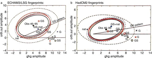
If two or more competing forcings are compared, the relative significance of the computed climate response signals can be compared in the plane or higher dimensional space spanned by the associated fingerprint patterns. Figure 1, from Barnett et al. (1999), illustrates the application of the optimal-fingerprint method to discriminate between the climate response to two different anthropogenic forcings: greenhouse-gas emissions (G) and a combination of greenhouse-gas and sulphate aerosol emissions (GS). Figure 1a and b shows the results obtained using the noise covariance matrices computed for the Max Planck and Hadley Centre climate models, respectively. The climate-change signal patterns themselves, prior to the transformation to optimal fingerprints, were computed using the climate models of the Hadley Centre, the Max Planck Institute and the Geophysical Fluid Dynamics Laboratory. The fact that most of the GS simulations lie within the 95% confidence ellipse of the natural variability, while most of the G simulations lie outside the ellipse, supports the hypothesis that the overestimation of the greenhouse warming by many climate models was due to the negligence of the (regionally dependent) cooling effect of sulphate aerosols.

Fig. 1 Computed climate response signals to greenhouse-gas emissions alone (G) and a combination of greenhouse-gas and sulphate aerosol emissions (GS), with associated 95% confidence ellipses, for climate simulations of the Hadley Centre, the Max Planck Institute for Meteorology and the Geophysical Fluid Dynamics Laboratory. Fingerprint patterns were computed using the climate models of MPIM (a) and the Hadley Centre (b). Most GS simulations lie within, most G simulations outside the relevant 95% confidence ellipses. Reproduced from Barnett et al. (1999).

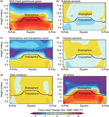
Most of the early detection and attribution analyses, as in the above example, were based on near-surface atmospheric temperature data, for which there exist relatively long time series and reasonably good global coverage. In recent years, the optimal-fingerprint approach has been extended to a wide variety of data sets, including upper layer ocean temperature, Arctic sea-ice extent, rainfall patterns, surface humidity, atmospheric moisture, continental river run-off and (Fig. 2) atmospheric vertical temperature distribution (see detailed review by Santer, 2010). This has provided exceptionally broad confirmation of the major anthropogenic contribution to recent climate change, as expressed in the increasing confidence in consecutive IPCC assessments, from the first 1995 statement that ‘The balance of evidence suggests a discernible human influence on global climate’ to the latest 2007 conclusion that ‘Most of the observed increase in globally averaged temperatures since the mid-20th century is very likely due to the observed increase in anthropogenic greenhouse gas concentrations’.

Fig. 2 Vertical profiles of temperature change for five different forcings and the resultant total force (f). The computed total change agrees well with observations. The decomposition confirms that most of the observed change is due to greenhouse-gas forcing – from Karl et al. (2009).

Qualifiers such as ‘very likely’ will continue to accompany detection and attribution statements until the anthropogenic signal has become so dominant (which we seek to prevent, however) that both questions have become scientifically irrelevant. The uncertainties arise, on the one hand, from the limitations of observational data, which are either of short duration (instrumental data) or provide only indirect information (proxy data), and on the other hand from the dependence on climate models, which are needed both to augment the observational data on natural variability and to compute the climate-change patterns in response to the external forcing. Despite the advances in climate modelling achieved with supercomputers, as evidenced by the realistic simulation of the large-scale regional structure and seasonal cycle of the global climate system, many processes, such as the formation of clouds, the occurrence of El Ninos, or smaller scale regional phenomena, are still not well understood.

The uncertainties increase if the detection and attribution method is applied to the impacts of climate change. The statistically robust conclusion that human activities have produced an observable change in climate rests strongly on global or large-scale regionally averaged data. The impact of anthropogenic climate change on society, however, is dominated by smaller scale or shorter term processes, such as changes in the frequencies and intensities of storms, floods and droughts, local water availability, or local sea-level rise. The demonstration that observed changes on these scales are indeed attributable to human activities is difficult to achieve with acceptable statistical significance because of the limited spatial resolution of global climate models and the relatively short period of the relevant instrumental data.

Nevertheless, changes in atmospheric circulation patterns, with attendant changes in the frequencies of extreme events, must be expected for a warmer climate, and they are indeed predicted by models. Although it is not possible to clearly attribute an individual extreme event to human activities, there is mounting evidence that, in their statistical accumulation, the observed increase in severe storms, major floods, extensive droughts and changes in the hydrological cycle can no longer be explained by natural variability alone. However, the evidence is uneven. Thus, whether tropical cyclones have increased in intensity or frequency, or have actually decreased in frequency (Sugi et al., 2009), remains a topic of controversy, while there is stronger evidence, for example, of an impact of climate change on the hydrological cycle (Held and Soden, 2006).

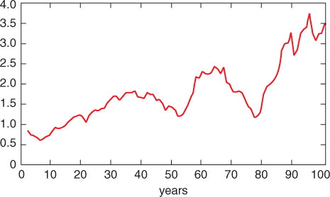
Another case of a probable anthropogenic climate-change impact is the occurrence of extreme heat events. Figure 3, from Coumou and Rahmstorf (2012), shows the temporal distribution of the maximal values of monthly-mean temperatures recorded over a period of a 100 yr at 17 stations worldwide. The monthly means are computed for each month of the year, yielding a total of 17×12=204 record values. In the absence of an anthropogenically induced trend or centennial-scale natural variability, the number of record-heat occurrences, as a function of time, would lie randomly distributed about a horizontal line. The observed upwards trend is strongly suggestive of an anthropogenic influence, although centennial-scale natural variability (as in all such investigations) cannot be ruled out.

Fig. 3 Ten-year averages of the number of monthly-mean heat records at 17 stations worldwide (corresponding to a total of 17×12=204 heat records).

The uncertainties encountered in the detection and attribution of anthropogenic climate change, extrapolated from the present into the future, are indicated qualitatively in Fig. 4. The latest business-as-usual (BAU) projections, based on the current accelerated use of fossil fuel, predict a global mean temperature increase by the end of this century of the order of 4°C (±50%) (World Bank, 2012), with up to twice these values over the continents. The predicted temperature increase is comparable to the warming since the last ice age, far exceeding the 2°C level generally accepted as the maximal tolerable global warming limit (see also the next section).

Fig. 4 Qualitative distribution of uncertainties associated with the detection, attribution, prediction and impact of climate change, with attendant widening risks.

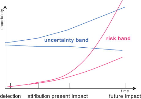
The uncertainties increase significantly the further one projects into the future. This is due not only to the growing divergence between the predictions of different climate models but also to significant differences between alternative projections of future greenhouse-gas emissions (IPPC, 2007). From the socio-economic planner's perspective, the uncertainties must be addressed in a risk-assessment framework. The challenge of the policymaker is not to respond to a well-defined predicted future climate state, or to wait (in vain) until science has resolved all uncertainties, but rather to develop appropriate policies to deal with a spectrum of possible evolution trajectories. The attendant uncertainties and risks must then be addressed in relation to a wider range of policy objectives.

3. Responding to climate change

Scientists have been warming of global warming since a continuous CO₂ monitoring station installed in 1957 on Mauna Loa by Charles Keeling (with the support of Bert Bolin) started measuring a stable, continuous rise in annual-mean atmospheric CO₂ concentration (superimposed on an annual cycle representing seasonal vegetation changes). The predictions by scientists of the resultant future global warming, assuming a constant trend of the Keeling curve, have not changed significantly over the past 50 yr. The political response, however, has been slow and inadequate. Climate scientists have attempted to accelerate the political process by collaborating with economists in constructing integrated assessment models to explore alternative paths for achieving a low-carbon global economy (IPCC, Working Group 3, 2007).

The challenge of achieving a transition to a low-carbon global economic system is illustrated in Fig. 5 by the wedge (Pacala and Socolow, 2004) separating a typical ‘BAU’ path of greenhouse-gas emissions (expressed in terms of CO₂ equivalent gigatonnes of carbon, IPPC, 2007), and a ‘sustainability path’, in which the global warming remains below 2°C. The 2°C ‘guard-rail’, based on the ‘tolerable windows approach’ of Bruckner et al. (1999), was proposed by the German Scientific Advisory Committee on the Environment (on the initiative of John Schellnhuber) shortly after the Rio 1992 UN Conference on the Environment and Development, as a realistic political constraint imposed by the UNCED commitment to avoid ‘dangerous climate change’ (Schellnhuber, 2010). It was accepted first by the European Union and later at COP15 (the 15th session of the Conference of Parties to the UN Framework Convention on Climate Change) in Copenhagen in December 2009 (although not matched by realistic commitments).

Fig. 5 Closing the wedge between a typical business-as-usual (BAU) greenhouse-gas emission path and a sustainability path that remains below the 2°C global warming guard rail. Renewable-energy technologies are ordered with respect to present costs. Solar energy is the largest, essentially unlimited, resource.

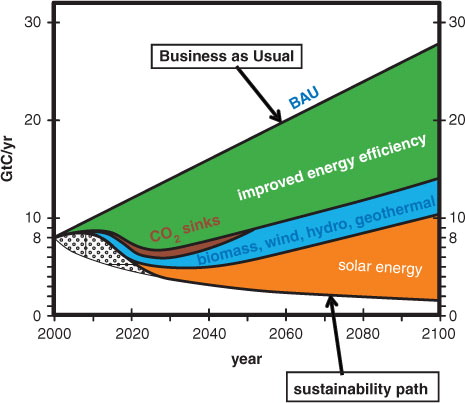
The figure shows a possible combination of technologies for closing the gap, beginning with the lowest (essentially zero or even negative) cost option of more efficient energy use and ending with the (currently) more expensive but essentially unlimited option of solar energy.

There exists widespread agreement among experts that, technically, the global energy system can be completely decarbonised during this century without exceeding the 2°C warming limit by applying renewable-energy technologies that are available already today. It is also generally accepted that the global costs of avoiding dangerous climate change are significantly lower than the potential costs, with attendant incalculable risks, incurred by unmitigated global warming (Stern, 2007).

Unfortunately, however, these conclusions have not led to an appropriate political response. There are many interpretations of the failure of COP-15 and its implications for the relation between science and policy (Schellnhuber, 2010). However, a major contribution was undoubtedly the global financial crisis of the previous year, which – in addition to the distraction of an urgent new global problem – had undermined the credibility of the main-stream economic models and the traditional utility-optimising cost-benefit analyses on which most of the integrated assessment models had been based.

Thus, there is a need for scientists to construct a new generation of integrated assessment models based on more realistic representations of the socio-economic-financial system. The communication with stakeholders and decision makers also needs to be improved. This requires the construction of simpler, more easily understandable models that address the issues of the current political debate in terms of concepts familiar to policy makers (Giupponi et al., 2013).

A basic difficulty, however, is that there exists today no consensus within the economic community on how the socio-economic-financial system actually works. The prevalent pre-2008 picture of a basically stable system, that adjusts automatically to an equilibrium growth path if left to the shock-absorbing forces of the free market, has fallen into disrepute through the financial crisis. Widespread agreement exists only that Adam Smith's ‘invisible hand’, that magically optimises a global inter-temporal utility function, needs to be replaced by a more realistic ensemble of competing socio-economic actors pursuing individual, normally conflicting, goals. The competing strategies of the different economic actors jointly determine the dynamic evolution of the system, which can then follow a wide variety of possible trajectories, depending on the individual actor strategies.

Since the appropriate game-theoretical integrated assessment models have yet to be developed, however, the traditional multi-regional, multi-sectoral general equilibrium models of the main-stream economic school have been replaced in the current political discussion by mental models based on intuitive concepts of the outcome of the competing strategies of the key economic players. Furthermore, the preoccupation with the global financial crisis and its repercussions such as the euro crisis, have focussed the political debate on these immediate issues, sidetracking the important long-term problems of climate change. However, we show below that the two problems are in fact intimately interconnected and need to be addressed in conjunction.

A translation of the competing mental pictures of the socio-economic-financial system that dominate the current political debate into quantitative, easily comprehensible actor-based, system-dynamic models, would shift the intuitive arguments over the most effective mechanisms for stabilising the system into the more objective arena of rational analysis. An illumination of the underlying multi-actor dynamics would then also point to the most promising paths towards decarbonising the global economy.

A new generation of integrated assessment models able to address these issues in the appropriate broader conceptual framework would need to include the following features:

1. A number of different actors (firms, workers, consumers, governments, banks, etc.) pursuing separate strategies to achieve their individual goals. In contrast to the single stable equilibrium of the main-stream efficient-market paradigm, interactions between several competing players can yield a wide variety of trajectories representing multiple quasi-equilibriums, exponential growth, catastrophic collapse, or continuous chaotic evolution. An understanding of the feedback processes underlying the game-theoretic structure of the multi-actor system is a necessary requirement for the implementation of effective economic regulation measures.

2. An explicit representation of the basic conflicts of interest between private and public goals. These arise both at the level of individual actors and at the international level of countries.

3. A realistic representation of the coupling of the financial sector to the production sector.

4. A generalisation of the concept of human value or happiness, including other factors besides the standard economic measure of GDP.

The purpose of such a multi-actor model system would not necessarily be to advocate a particular preferred policy but rather to provide a ‘canvas’ (Dietz et al., 2007) for painting alternative pictures of the socio-economic-political system as background for a quantitative analysis and discussion leading ultimately to a consensus.

As an example, we present in the following a series of model simulations summarising various views of the interrelation between the joint tasks of stabilising the financial system and decarbonising the economy.

3.1. A globally integrated green-growth model

Our simulations were performed with a modified version of the Multi-Actor Dynamic Integrated Assessment Model System MADIAMS (Weber et al., 2005; Hasselmann and Voinov, 2011; Hasselmann and Kovalevsky, 2013). The model was calibrated against so-called stylised facts (Maddison, 1982, 1995), where available, but is otherwise based on estimated interaction parameters.

The model is composed of two coupled modules: a production sector and a financial sector. We consider first the production module.

3.1.1. The production module

The total production y is decomposed into three components and y _g representing the production of fossil-energy-based capital k, renewable-energy-based capital r, and consumer goods and services, g (Fig. 6). The input flows to the stocks r,k,g are offset by outflows representing capital depreciation and the consumption of consumer goods and services. The production streams provide no direct contribution to the production of consumer goods and services – the ultimate purpose of the economy – but generate rather the renewable and conventional capital components r,k that are needed as input to the production function itself: y=y(r,k).

Fig. 6 Vensim-software sketch (cf. http://www.vensim.com) of the stocks (boxes) and flows (choke valves – or hour glasses) of a simple real-economy model (see text). Details of the actor-dependent variables controlling the stocks and flows are not shown.

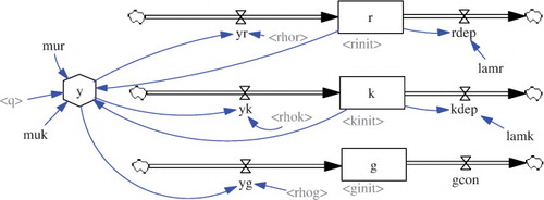
We have assumed the simple form , where q is the employment level, µ _k is a constant and µ _r is a gradually increasing function of y _r that simulates the learning-by-doing effect of a new technology.

The employment level q is determined by the strategy of the economic actors (firms, households, governments, banks) in response to market signals, such as prices, wage levels and taxes. These are modelled in the financial sector, considered in the next section. To illustrate the basic dynamics of the production sector, independent of the financial sector, we assume in this section full employment, q=1.

The term ‘capital’ is used here in a general form, encompassing physical and human capital (education, job experience, etc.) as well as institutions (legal and administrative system, business culture, constitution, government structure, etc.). The formal division of capital into conventional-energy and renewable-energy-dependent components is based on an estimate of the relevant contributions of these two energy input components into the production function, under the basic assumption that the creation of all outputs of the economy involves ultimately some form of energy input.

The evolution of the system is governed by distribution factors that describe the decomposition of the total production y into three streams: , with .

Figures 7 and 8 show as an example the distribution factors and associated GDP growth curves, respectively, for a BAU scenario and green-growth scenario GREEN. Both scenarios assumed the same constant fraction for the investment in consumer goods and services. The BAU scenario included no investments in renewable energy, , while in the simulation GREEN, the fraction ρ _r was gradually increased relative to the fraction ρ _k , ensuring that the global warming remained below 2°C (Fig. 9, upper panel).

Fig. 7 Evolution of production-distribution factors for the simulations BAU (ρ _r =0, ρ _k =0.65, ρ _g =0.35) and GREEN (green curve, with ρ _g =0.35 and ρ _r /ρ _k monotonically increasing).

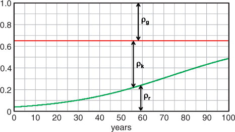
Fig. 8 Computed growth of GDP for a business-as-usual scenario (blue) and a reduced-emission scenario (green) for which the global warming remains below 2°C. (GDP is represented in arbitrary currency units ‘$’/year). Mitigation measures incur a growth delay over a period of 100 yr of only a few years.

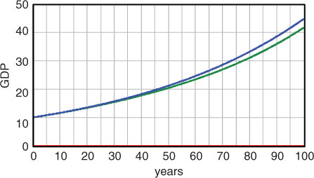
Fig. 9 Impact of the two scenarios BAU (blue) and GREEN (green) on global mean temperature (a) and welfare (b).

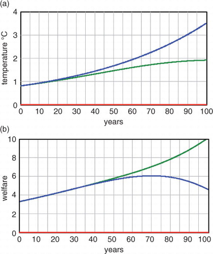
The simulations support the consensus view of the feasibility and affordability of the transformation to a carbon-free economy. They are consistent with other investigations (e.g. Azar and Schneider 2002; IPCC, Working Group 3, 2007; Stern, 2007), all of which conclude that the slightly higher short-term costs of renewable energy are negligible compared with the longer term climate-damage costs of the BAU scenario. The loss of GDP incurred by effective mitigation policies incurs an acceptable delay of economic growth of only a year or two over a period of 100 yr.

The impact of the two scenarios on climate (expressed in terms of the global mean temperature increase T) and human welfare w is shown in Fig. 9. The temperature increase was computed using a simplified version of the non-linear impulse response climate model NICCS (Hooss et al., 2001) from the CO₂ emissions generated by the production y _k in the fossil-energy sector.

Welfare is represented in our model by the simple expression1

Since full employment, q=1, was assumed in the simulations shown, the welfare expression reduces to the product of the production y _g of consumer goods and services and a climate impact factor analogous to the expressions assumed by other authors (Nordhaus, 1994; Weber et al., 2005; Stern, 2007).

The joint impact of economic evolution and climate change on human ‘welfare’ necessarily involves a subjective value assessment. Generally accepted is only that welfare depends not only on GDP (y – or, more appropriately, the production y _g of consumer goods and services) but also on many other factors, such as health insurance, unemployment levels, job security, crime level, income inequalities, pension guarantees, and – of particular relevance in the present context – the state of the present and future environment. Our simple welfare expression (1) represents the projection of a host of important societal and environmental parameters onto three selected key variables, y _g , q and T. The variables are chosen in anticipation of a high correlation of the full welfare function; however, it is defined with these variables for our particular set of simulations. The fact that we have not attempted to substantiate our simple, subjective welfare expression by data emphasises the need for a translation of the many sociological investigations of the welfare concept into numbers that, however controversial, can be incorporated into integrated assessment models.

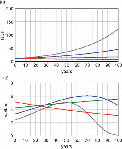
The pronounced loss in welfare of the BAU scenario compared to the scenario GREEN in Fig. 9 could conceivably have been exaggerated in our example by an exceptionally low welfare value of the chosen BAU scenario. That this is not the case is demonstrated in Fig. 10, which compares the simulation BAU (ρ _k =0.35) with three bracketing simulations BAU₁, BAU₂, BAU₃, with ρ _k =0.25, 0.45, 0.55, respectively. The reference BAU scenario is seen to exhibit the highest relative welfare values.

Fig. 10 Evolution of GDP (a) and welfare (b) for four BAU scenarios corresponding to ρ _k =0.25, 0.35, 0.45, 0.55, with ρ _r =0 in all cases. The reference scenario BAU (blue), with ρ _k =0.35, yields the highest welfare values.

The reproduction of these basically well-known economic growth relations with a simple system-dynamics model of the production sector of the economy emphasises two important points.

First, the conclusions are strongly dependent on unavoidable uncertainties and value assumptions. These follow, on the one hand, from the uncertainties of climate predictions and future economic growth, as discussed earlier, and, on the other hand, from the necessarily subjective nature of the welfare concept. This depends, in addition to the factors mentioned, on the weighting of future welfare relative to the present welfare. We have not attempted to represent this through a discount factor, a long-standing subject of debate (see, e.g. Nordhaus, 1997; Hasselmann, 1999, and the more recent controversy, Tol and Yohe, 2006; Nordhaus, 2007, over the low discount factor used in the Stern (2007) review). The root of the controversy lies ultimately in the conflict between private and public goals: the short time scales of private investors seeking a rapid return on investment are incompatible with the longer time horizon of governments concerned with preserving a habitable planet for future generations. Since the task of policy makers is to balance these two legitimate objectives, modellers need to explicitly include the alternative private-versus-public weightings of future relative to present welfare in their integrated assessment models.

Second, the evolution of the economy is governed by the strategies of the economic actors that determine the employment level q and the distribution of total production between the three production streams . In contrast to the general consensus on the technical feasibility and affordability of decarbonisation, there exists no widespread agreement on the most effective policies for promoting investments in low-carbon technology. Investments depend on actor decisions, which can result not only in green growth but also in major instabilities, such as the financial crisis. The goal of decarbonisation is thus closely connected to the task of stabilising the coupled economic-financial system. Both require an improved understanding of actor behaviour. This is governed by market signals generated in the financial sector, the second module of our coupled system.

3.1.2. The financial module

The stocks-and-flows representation of the financial module is summarised in Fig. 11. The evolution of the coupled system is governed by the strategies of five representative economic actors: a firm, a household, a government, an investor and a central bank. To distinguish between the investment streams in carbon-based and renewable-based capital stocks, each firm and investor is further subdivided into two actors, yielding a total of seven formally independent actors.

Fig. 11 Vensim-software sketch of the module representing the financial system coupled to the production module of Fig. 6. Money stocks and flows assigned to firms and investors are separated into renewable-energy-related liquidity and assets (left) and fossil-energy-related liquidity and assets (right). Details of the various inputs to the stocks and flows are not shown.

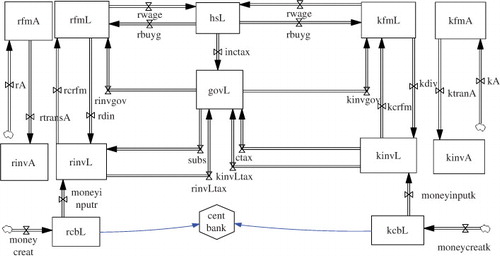
The complete model consists then of 12 state variables: three for the production sector (conventional and renewable-based capital r, k and consumer goods and services g), and nine for the financial sector: seven representing the actor liquidities (hsL, govL, kinvL, rinvL, kfmL, rfmL, cbL) plus two state variables for the assets (kinvA, rinvA) owned by investors. It is assumed that, with the exception of investors, who own the capital assets of the firms in which they have invested, the wealth of all actors is expressed solely in terms of liquidity. The role of the central bank is to create new money in response to the expansion of the economy. This is achieved by satisfying the money demand of investors, which therefore act indirectly as the originators of new money by providing credit to firms.

We note that we use the term ‘actor-based’ here rather than ‘agent-based’ to emphasise that our actors refer to real economic players, rather than agents in a wider sense, which can represent either actors as defined here (Li, 2011) or abstract modules interacting with other modules in a numerical simulation model (Tesfatsion, 2006).

We have not addressed the interesting question of the extent to which, in a non-linear system, the emergent net impact of the behaviour of a large number N of heterogeneous actors of a given functionality can be represented by an average representative actor (Kirman, 1992; Beinhocker, 2006; Gintis, 2007; Farmer and Foley, 2009; Mandel et al., 2009). In our applications we have assumed, in effect, that the closure from large N (≈100–1000) to small N (=7) can be achieved by heuristic arguments, as in phenomenological thermodynamics or turbulence theory. We note in this context that the term ‘multi-actor’ in the acronym MADIAMS refers to ‘multiple actors’, as opposed to the benevolent single actor of the efficient-market paradigm. It should be distinguished from the term ‘multi-agent’ (often used synonymously with ‘agent-based’) in the sense of a ‘multitude of agents’, as applied to large, N agent-based models.

The evolution of the financial system in this system is governed by the money transfers between nine state variables. The money flows, in turn, depend on a number of actor-dependent ‘transfer’ parameters, namely: the wages negotiated between firms and wage earners (households), the fraction of wages saved by households rather than being spent on consumer goods, the purchase of capital assets from firms by investors, the dividends investors receive from firms, the prices of consumer goods and capital assets, the income tax and carbon taxes imposed by the government, the recirculation of the tax income to firms in the form of investments and subsidies, and – a particularly important variable that enters as a factor in all transfers involving households as well as in all production variables – the employment level.

Thus the system equations, in both modules, consist of two classes: conservation equations and actor strategies. The first represent simple stocks-and-flows balance equations for goods (production sector, Fig. 6) and money (financial sector, Fig. 11). The second represent actor–strategy relations that determine the production streams and the employment level, in the production sector, and the various money streams between actors, in the financial sector. The actor strategies are also governed by non-linear ordinary differential equations that can be visualised in (non-conservative) stocks-and-flows diagrams (not shown).

Our model, despite its numerous interconnections, is clearly a highly idealised representation of the real, socio-economic-financial system. Nevertheless, it already captures many of the actor-dependent dynamical features observed in real systems. These can be either stabilising or destabilising, as opposed to the inherent stability assumed in main-stream general equilibrium models. For the following, the details of the model (specified, e.g. in alternative realisations in Weber et al. 2005; Hasselmann and Voinov, 2011 and Hasselmann and Kovalevsky, 2013) are irrelevant. The emphasis here is on the model's basic dynamic structure and the controlling role of actor behaviour.

We consider in the following a series of model simulations (Table 1) differing in the assumed actor response to market signals. The models can be divided into two classes: supply-driven models S and supply-demand-feedback models F.

Table 1. Model runs of the coupled production-financial sectors, classed into supply-driven models S and supply-demand-feedback models F

Model	Class	Properties
BAU	S	Business-as-usual
GREEN	S	Green investment
BAL	S	BAU, balanced budget
DEF	S	BAU, deficit budget
SAV	F	BAU, savings policy Balances budget
REC	F	BAU, savings policy creates recession
GR-INV	F	Green investments balance budget and create growth

In supply-driven models, the production sector of the economy is decoupled from the financial sector. This permits the realisation of the same real economic growth trajectory for quite different trajectories of the liquidities and assets of the actors in the financial sector. Although highly implausible from the viewpoint of formal economic theory, the situation corresponds rather closely to reality, as manifested by the prevalence of unbalanced national budgets.

Supply-demand-feedback models include the feedback of the financial sector on the production sector. These feedbacks become particularly relevant when economic actors and policy makers strive to restore balanced-budget trajectories, starting from diverging unbalanced budgets.

3.1.3. Supply-driven systems

The simulations BAU, GREEN and BAU_1,2,3 represented supply-driven systems limited to the production sector, but were nevertheless carried out for intercomparison purposes using the full coupled model. The production sector was decoupled from the financial sector through the prescription of the three production stream ratios, together with the market-clearing assumption that the production and consumption of consumer goods and services adjusted immediately to prescribed ratios consistent with exponential growth.

The BAU simulations, with constant coefficients and with ρ _r =0, were characterised by particularly simple dynamics. The general solution consists of a superposition of two eigen solutions: an exponentially growing solution and an exponentially decaying solution , with positive constants . (There exist only two eigen solutions, as the side condition ρ _r +ρ _k +ρ _g =1 establishes a linear dependence between the three state variables.) The exponentially growing solution represents a stable attractor (an ‘equilibrium’ in standard economic terminology).

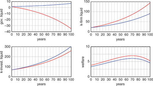
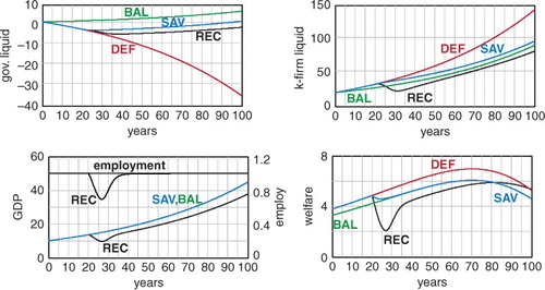
The existence of many possible solutions for the financial sector for a single solution of the economic sector is illustrated in Fig. 12, which compares two alternative financial-sector solutions BAL and DEF given the solution BAU of the economic sector. The solution BAL represents a balanced financial system, characterised by a common exponential growth ~ of all variables of the financial sector, consistent with the exponential growth rate of the production sector. The simulation DEF represents an unbalanced solution characterised by a deficit government budget. The asymptotic growth rate is again exponential for all financial-sector variables, with the same common exponential factor ~ as in the case BAL, but now with negative amplitude for the government liquidity. (The remaining 11 eigenvectors of the system consist of the exponentially decaying component ~ of the BAU case and ten constant components.)

Fig. 12 Alternative evolutions of the financial sector of the model MADIAMS for the same evolution BAU of the real-economy sector. The scenario BAL (blue) corresponds to balanced wealth growth of all economic actors commensurate with real economic growth, while the government-deficit scenario DEF (red) yields higher but non-sustainable values of household welfare and firm liquidity, at the cost of increasing government deficits.

The government debt in the simulation DEF is assumed to be financed by investors. The money inflow from investors is transferred from governments to firms through government contracts. (The role of governments in redistributing wealth between different income groups is not resolved in our highly aggregated model.) The firms, in turn, partially transfer the enhanced income to households in the form of higher wages. Interest payments by the government are not represented as a separate money stream, since, for exponential growth, they enter simply as a factor partially offsetting the credit uptake.

It is assumed that the additional credit supplied by investors to governments is not balanced in the simulation DEF by an additional money uptake of the investors from the central bank. Thus, the total wealth of the system is the same in both the balanced-budget case BAL and the deficit-budget case DEF.

Welfare, as defined in eq. (1), also remains unchanged, as the total production, the distribution of production and the assumption of full employment, remain the same. This is, of course, unrealistic in view of the increased household income in the deficit-budget case. It follows formally because, for a closed economy with a given level of production and consumption of consumer goods and services, an increase in household income can lead only to an increased level of household savings (liquidity), which is not included in our simple welfare definition (1). We assume therefore in the deficit-budget case, more realistically, that the increase δi of the household income produces an increased consumption level through the purchase of imports from a foreign economy. This can be expressed by replacing y _g in the welfare expression (1) by , yielding the welfare curve shown in Fig. 12 (bottom right).

The enhanced welfare of the deficit model is sustainable only as long as investors are willing to accept an increasing outstanding government debt, and the foreign economy maintains the trade imbalance . At some point, however, the investors will balk, and an attempt will be made to adjust the economy to the balanced-growth path of the scenario BAL. Views on the best policy for achieving the transformation differ, depending on the assumed actor response.

If one adheres to the traditional main-stream paradigm of an inherently stable economic system, the recipe is straightforward: one simply adjusts the government expenditure and tax income such that they match, and the economy will automatically adjust to the balanced-budget growth path BAL. This is shown in the simulation SAV (Fig. 13, blue curves). The budget corrections were applied 20 yr after the beginning of the deficit growth path, with an assumed adjustment time constant of 3 yr. The welfare level falls back to the reference BAU curve, as intended, without major repercussions for the economy.

Fig. 13 Alternative predictions of the impact of strict saving measures to adjust the deficit-budget evolution path DEF (red curves) to the balanced-budget growth path BAL (green curves). The simulation SAV (blue curves) assumes a monotonic relaxation to the balanced-budget path, while the simulation REC (black curves) predicts a severe recession with major unemployment.

3.1.4. Supply-and-demand-feedback systems

This is not, however, what is typically experienced. Austerity policies in most cases lead to major recessions and unemployment (as observed in the southern European countries in the present euro crisis). To reproduce these alternative outcomes (Fig. 13, simulation REC, black curves), the model needs to be generalised to include a wider spectrum of actor behaviour than assumed in the efficient-market paradigm of the simulation SAV. In particular, the feedback of variations in demand on the supply needs to be considered.

In standard macro-economic text books (Samuelson and Nordhaus, 1995; Abel and Bernanke, 2005) the self-stabilising forces of the market are typically presented in terms of the familiar diagonal-cross diagram of the supply and demand curves in the price–quantity plane: any externally imposed change in demand, supply or price from the equilibrium crossing point is assumed to induce stabilising restoring forces that return the system to a new equilibrium point. However, business cycles, boom-and-bust events in asset markets, random fluctuations in the stock market and the collapse of the global financial system are evidence that economic actors do not necessarily conform to this main-stream picture.

Three de-stabilising actor feedbacks are frequently encountered. An increase in the price of an asset, instead of inducing a stabilising decrease in demand, can stimulate an increase in demand for investors anticipating a further rise in the value of the asset (Mackay, 1852/1995; Soros, 2008). Modern financial products, such as collatorised debt obligations (DBOs) and credit default swaps (CDSs), although distributing risk (a desirable factor), at the same time greatly enhance total risk by inviting individual investors to engage in risks they would otherwise not have undertaken – a problem widely discussed in relation to the causes of the financial crisis. Finally, a decrease in the demand of consumers, rather than encouraging a stabilising decrease in price by producers, can induce firms to reduce production. This decreases consumer income and thereby further demand, leading to a recession or business cycle – also a prominent theme of public concern with respect to the appropriate response to the financial crisis.

The impact of boom-and-bust events and business cycles on long-term economic growth has been investigated in the context of climate-change mitigation policies in Hasselmann and Kovalevsky (2013). In the following, we apply the feedback dynamics of recessions to the example of sovereign debt.

We assume in our simulation REC that the response of firms to government policies seeking to balance the budget by reducing the wages of government employees, or postponing infra-structure investments, is not to lower prices, but rather to reduce the supply by laying off workers. The unstable, positive feedback leading to an exponential collapse of the economy is finally arrested through the reduction of wages to a level at which firms again become willing to employ workers.

The impact of the reduced employment level q enters linearly in the overall production y, but quadratically in our assumed expression (1) for the welfare w (through the linear dependence of w on y _g and, additionally, on q directly). This results in a pronounced decrease in welfare (simulation REC, Fig. 13, bottom right), which persists until it is finally compensated by the reduced climate warming associated with the reduced CO₂ emissions of the depressed economy.

The rise in unemployment can be avoided if the necessary reduction of the workforce in the sector of consumer goods and services is compensated by the hiring of workers in a new production sector. An obvious candidate is the accelerated expansion of renewable-energy technology. Figure 14 (green curves) shows the results for the simulation GR-INV, in which the fraction ρ _r of total production invested in renewable-energy capital is increased relative to the fraction assumed in the earlier greening simulation GREEN (Figs. (7–9)). The increase in ρ _r is introduced after t=20 yr, coincident with the budget-balancing reduction in government transfers to the fossil-capital sector of the economy, which is applied as before.

Fig. 14 Interrelation between decarbonisation and stabilisation of the financial markets. Simulation GR-INV (dark green curves) shows the impact of government savings measures accompanied by enhanced Keynesian investments in renewable energy. Simulation REC (black curves) shows the impact of savings measures alone, leading to a recession. Also shown is the original decoupled real-economy decarbonisation simulation GREEN (light green curves).

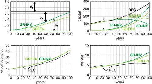
The initial decrease in welfare is minor, and comparable with the decrease computed in the previous (unrealistically optimistic) simulation SAV (Fig. 13). Despite the shift of investments from consumption goods to green technology, the resultant welfare values lie very close to the GREEN curve in the medium term, and exceed these in the long term.

4. Conclusions

Extensive research on observed climate change following initial estimates of the signal-to-noise ratio in the early 1990s has today clearly established the dominance of the human influence over natural climate variability on global scales. However, whether the climate change observed on regional scales, such as increases in the frequency or intensity of storms, droughts, heatwaves and other extreme events, can be clearly attributed to human activities rather than decadal scale natural variability remains in many cases an open question. Since these are the climate-change phenomena that are predicted to strongly affect future human living conditions, society cannot afford to wait until the anthropogenic signal has clearly risen above the natural variability noise also on these scales before implementing effective mitigation and adaptation policies to counter the unabated emission of greenhouse gases.

To support policy makers in the implementation of effective climate policies, climate scientists need to collaborate with economists to produce more realistic coupled climate-socio-economic models that are able to better assess the impact of alternative policies. Unfortunately, climate policy has stagnated in recent years through the preoccupation with the financial crisis. This has been aggravated by the failure of the economic profession to foresee the crisis, which has led to a loss of credibility of the main-stream economic models on which many of the past assessments of climate policies have been based. Needed is a new generation of actor-based, system-dynamic integrated assessment models that address within the same model the instabilities that led to the financial crisis and the policies needed to initiate a green transformation.

We have presented a simple, model system and a number of simulations based on these concepts. None of the processes we have investigated are new. But the political debate on the resolution of the global financial crisis, with its more regional dislocations such as imbalances within the euro region, has lacked hitherto a translation into simple, easily understandable simulation models. These are necessary not only for the verification or falsification of the proposed mental models through quantitative comparisons against data, but already at a more fundamental level to test the internal consistency of the (often non-trivial stocks-and-flows) implications of the mental models.

We have discussed in more detail one particular example: the resolution of the current euro crisis through the transformation of the European economy to a low-carbon system, thereby avoiding the creation of severe recessions and high unemployment. However, the actor-based, system-dynamic modelling approach, using easily implemented and interpretable modern graphic software, can be readily applied to many other coupled environment-socio-economic problems.

The application of such models in a global framework would broaden this focus on the global financial crisis to the important longer term challenge of creating a global carbon-free economy. Both tasks are intimately interconnected. The greening of the global economy requires major long-term investments. These will be forthcoming only if investors have confidence in the stability of the system in which they are investing. Conversely, the stability of the socio-economic-financial system can be strengthened by government policies promoting investments in carbon-free technologies.

5. Acknowledgments

Ben Santer and Gabi Hegerl provided valuable inputs on recent developments in the field of detection and attribution. Dmitry Kovalevsky collaborated in the development of earlier versions of the MADIAMS model hierarchy. Support from the Max Planck Institute for Meteorology, the Global Climate Forum and the EU projects GSDP, EURUCAS and COMPLEX is gratefully acknowledged.

Notes

¹The VENSIM code of the MADIAMS model system can be downloaded from the website of the Global Climate Forum, http://www.globalclimateforum.org/.

References

- Abel A , Bernanke B . Macroeconomics. 2005; Boston: Pearson Addison Wesley.
- Arrhenius S . On the influence of carbonic acid in the atmosphere on the temperature of the ground. Phil. Mag. 1896; 41: 237–276.
- Azar T , Schneider H . Are the economic costs of stabilizing the climate prohibitive?. Ecol. Econ. 2002; 42: 73–80.
- Barnett T , Hasselmann K , Chlliah M , Delworth T , Hegerl G , co-authors . Detection and attribution of recent climate change: a status report. Bull. Am. Meteorol. Soc. 1999; 80: 2631–2659.
- Beinhocker E . The Origin of Wealth. 2006; Boston: Harvard Business School Press.
- Bruckner T , Petschel-Held G , Toth F , Fssel H , Helm C , co-authors . Climate change decision-support and the tolerable windows approach. Environ. Model. Assess. 1999; 4: 217.
- Coumou D , Rahmstorf S . A decade of weather extremes. Nat. Clim. Change. 2012; 2: 491–496.
- Dietz S , Hope C , Patmore N . Some economics of dangerous climate change: Reflections on the Stern Review. Global Environ. Change. 2007; 17: 311–325.
- Farmer D , Foley D . The economy needs agent-based modelling. Nature. 2009; 460: 685–686.
- Fourier J . Remarkes générales sur les températures du globe terrestre et des espaces planétaires. Annales de Chemie et de Physique. 1824; 27: 136–167.
- Gintis H . The dynamics of general equilibrium. Econ. J. 2007; 117: 1280–1309.
- Giupponi C , Borsuk M , de Vries B , Hasselmann K . Innovative approaches to integrated global change modelling. Ecol. Model. Software. 2013; 4: 1–9.
- Hasselmann K . Stochastic climate models, part 1: theory. Tellus. 1976; 28: 473–485.
- Hasselmann K , Shaw G. B . On the signal-to-noise problem in atmospheric response studies. Meteorology of Tropical Oceans. 1979; Bracknell: Royal Meteorological Society. 251–259.
- Hasselmann K . Optimal fingerprints for the detection of time-dependent climate change. J. Clim. 1993; 6: 1957–1969.
- Hasselmann K . Intertemporal accounting of climate change-harmonizing economic efficiency and climate stewardship. Climatic Change. 1999; 41: 333–350.
- Hasselmann K , Kovalevsky D . Simulating animal spirits in actor-based environmental models. Environ. Model. Software. 2013; 44: 10–24.
- Hasselmann K , Voinov A , Jaeger C , Hasselmann K , Leipold G , Mangalagiu D , Tabara J. D . The actor driven dynamics of decarbonization. Reframing the Problem of Climate Change. From Zero Sum Game to Win-Win Solutions. 2011; New York: Earthscan. 131–159.
- Hegerl G , von Storch H , Hasselmann K , Santer B , Cubasch U , co-authors . Detecting greenhouse gas-induced climate change with an optimal fingerprint method. J. Clim. 1996; 9: 2281–2306.
- Held I , Soden B . Robust responses of the hydrological cycle to global warming. J. Clim. 2006; 19: 5686–5699.
- Hooss G , Voss R , Hasselmann K , Maier-Reimer E , Joos F . A Nonlinear Impulse response model of the coupled Carbon-cycle-Climate System (NICCS). Clim. Dynam. 2001; 18: 189–202.
- IPCC, Working Group 3. Climate Change 2007, Mitigation of Climate Change, Intergovernmental Panel on Climate Change, Fourth Assessment Report. 2007; Cambridge: Cambridge University Press.
- IPPC. Intergovernmental Panel on Climate Change. 2007; Cambridge: Fourth Assessment Report. Cambridge University Press.
- Karl T , Melillo J , Peterson T . Global Climate Change Impacts in the United States. 2009; Cambridge.: Cambridge University Press.
- Kirman A. P . Whom or what does the representative individual represent?. J. Econ. Perspect. 1992; 6: 117–136.
- Li A . Modeling human decisions in coupled human and natural systems: review of agent-based models. Ecol. Model. 2011; 229: 25–36.
- Mackay C . Extraordinary Popular Delusions and the Madness of Crowds. 1852, republished 1995; Wordsworth Editions, Ware, UK.
- Maddison A . Phases of Capitalist Development. 1982; Oxford University Press, Oxford.
- Maddison A . Monitering the World Economy. 1995; Paris: OECD.
- Mandel A , Fürst S , Lass W , Meissner F , Jaeger C . Lagom Generic: An Agent-Based Model of Growing Economies. 2009; Berlin.: ECF working paper 1/2009. Technical Report, European Climate Forum.
- Meadows D , Meadows D , Randers J , Behrens III W. . The Limits to Growth. 1971; New York: Potomac Associates.
- Nordhaus W . Managing the Global Commons: The Economics of the Greenhouse Effect. 1994; Boston: MIT Press.
- Nordhaus W . Discounting in economics and climate change; an editorial comment. Climatic Change. 1997; 37: 315–328.
- Nordhaus W . A review of the Stern Review on the Economics of Climate. J. Econ. Lit. 2007; 45: 668–702.
- Pacala S , Socolow R . Stabilization wedges: solving the climate problem for the next 50 years with current technologies. Science. 2004; 305: 968–972.
- Samuelson P , Nordhaus W . Economics. 15th ed . 1995; New York: McGraw-Hill.
- Santer B. Testimony at hearing on “A rational discussion of climate change: The science, the evidence, the response.”. US House Committee on Science and Technology, Subcommittee on Energy and Environment. 2010. House of Representatives, Serial No. 111–114, http://www.science.house.gov.
- Santer B , Brggemann W , Cubasch U , Hasselmann K , Höck H , co-authors . Signal-to-noise analysis of time-dependent greenhouse warming experiments. part 1: pattern analysis. Climate Dynam. 1994; 9: 267–285.
- Schellnhuber H . Tragic trimph. Climatic Change. 2010; 100: 229–238.
- Soros G . The New Paradigm for Financial Markets: The Credit Crisis of 2008 and What It Means. 2008; New York: Public Affairs, Perseus Books Group.
- Stern N . The Economics of Climate Change. The Stern Review. 2007; Cambridge: Cambridge University Press.
- Sugi M , Murakami H , Yoshimura J . A reduction in global tropical cyclone frequency due to global warming. SOLA. 2009; 5: 164–167.
- Tesfatsion L , Colander D . Computational modelling and macroeconomics. Post Walrasian Macroeconomics. 2006; Cambridge: Cambridge University Press. 175–202.
- Tol R , Yohe G . A review of the Stern Review. World Econ. 2006; 7: 233–250.
- Tyndall J . Contributions to Molecular Physics in the Domain of Radiant Heat. 1873; New York: D. Appleton & Co.
- Weber M , Barth V , Hasselmann K . A multi-actor dynamic integrated assessment model (MADIAM) of induced technological change and sustainable economic growth. Ecol. Econ. 2005; 54: 306–327.
- World Bank. Turn down the heat: why a 4°C warming world must be avoided. 2012; World Bank, Washington, DC.